Abstract
Reasonably formulating the strawberry harvesting sequence can improve the quality of harvested strawberries and reduce strawberry decay. Growth information based on drone image processing can assist the strawberry harvesting, however, it is still a challenge to develop a reliable method for object identification in drone images. This study proposed a deep learning method, including an improved YOLOv8 model and a new image-processing framework, which could accurately and comprehensively identify mature strawberries, immature strawberries, and strawberry flowers in drone images. The improved YOLOv8 model used the shuffle attention block and the VoV–GSCSP block to enhance identification accuracy and detection speed. The environmental stability-based region segmentation was used to extract the strawberry plant area (including fruits, stems, and leaves). Edge extraction and peak detection were used to estimate the number of strawberry plants. Based on the number of strawberry plants and the distribution of mature strawberries, we draw a growth chart of strawberries (reflecting the urgency of picking in different regions). The experiment showed that the improved YOLOv8 model demonstrated an average accuracy of 82.50% in identifying immature strawberries, 87.40% for mature ones, and 82.90% for strawberry flowers in drone images. The model exhibited an average detection speed of 6.2 ms and a model size of 20.1 MB. The proposed new image-processing technique estimated the number of strawberry plants in a total of 100 images. The bias of the error for images captured at a height of 2 m is 1.1200, and the rmse is 1.3565; The bias of the error for the images captured at a height of 3 m is 2.8400, and the rmse is 3.0199. The assessment of picking priorities for various regions of the strawberry field in this study yielded an average accuracy of 80.53%, based on those provided by 10 experts. By capturing images throughout the entire growth cycle, we can calculate the harvest index for different regions. This means farmers can not only obtain overall ripeness information of strawberries in different regions but also adjust agricultural strategies based on the harvest index to improve both the quantity and quality of fruit set on strawberry plants, as well as plan the harvesting sequence for high-quality strawberry yields.
1. Introduction
Strawberries are edible fruits in high demand worldwide, with high economic and nutritional value [1]. Most varieties of strawberries have a short duration of maturity, transitioning from white maturity to complete maturity after about 7 days [2]. The suitable harvesting time for mature strawberries is only 1–3 days, which leads to different ripening times for strawberries in the same area of large-scale farmland and requires batch harvesting [3]. Failure to harvest in a timely manner will lead to excessive maturity of strawberries, decreased overall quality, and easy decay [4]. Strawberry growers need to frequently observe the growth of strawberries in farmland to plan harvesting decisions [5]. Therefore, it is necessary to study a method to quickly obtain the overall growth information of strawberry fields during the harvesting stage, provide growth status information, assist in planning the harvesting plan, ensure that strawberries are harvested in a timely manner at the appropriate stage during the peak harvest period, and improve product quality.
In recent years, strawberries have been mainly cultivated in large strawberry fields, using modern technology to achieve a large-scale, efficient, and scientific planting mode. During the planting stage, transplanters are often used in the transplanting process of strawberry seedlings [6]. During the growth stage, various sensors are used to monitor soil, air, and other data to assist in the growth of strawberries. During the harvesting stage, a robot applies automatic obstacle avoidance algorithms [7]. In harvesting tasks [8,9], drones can be used for tasks such as yield prediction and crop mapping [10]. Compared to the ground vehicle, the images obtained by drones have advantages, such as high resolution, panoramic perspective, and efficient coverage, which helps to achieve wide-area and high-precision spatial data acquisition.
The images captured by drones have the problem of many targets to be detected and small target sizes. The main solution is to increase the number of detection pyramid layers; however, this will weaken the representation of details in low-level features and increase the model size [11]. Deep learning can learn the growth patterns of crops, and efficiently and accurately identify the types and positions of crops, and is widely used in the field of digital image recognition [12]. In practical applications, it is often necessary to improve the structure of the deep learning model according to crop characteristics. Backbone networks, attention mechanisms, and loss functions are common improvement parts of the deep learning model. The DSE (detail–semantics enhancement) module, which uses dilated convolution, effectively addresses the maturity detection issue for small target strawberries [13]. VGG-16 was replaced by an improved multi-cascade network structure in the Faster R-CNN module, achieving precise recognition and counting of strawberries [14]. Wise iou is a loss function that can accelerate convergence speed. By applying it to the YOLOv7 model, occluded strawberries of small targets are effectively recognized [15].
After object detection in RGB images is captured, it is usually necessary to determine the distribution, density, and overall growth stage information of crops according to the target detection results. Applying Bayesian inference methods to the processing of strawberry detection results enables the prediction of strawberry yield in the strawberry field [16]. Jointing the aerial orthoimages recognized by FasterR-CNN allows for the effective visualization of the overall yield in the strawberry field [17]. By identifying strawberry flowers and berries in drone images, Zhou achieved near-term growth predictions for the strawberry field [18]. Collecting environmental data during strawberry growth using various sensors and processing the data with machine-learning algorithms enables the indirect prediction of strawberry yield [19]. The premonition net is employed to learn strawberry recognition results from past, present, and future moments. Combined with the transform structure, it achieves the prediction of strawberry growth conditions [20].
Based on the above analysis, this study used a drone to capture RGB images of various regions in the entire strawberry field and focused on the obtaining method of strawberry growth information. The main contents of this study are as follows:
- An improved YOLOv8 model was proposed to recognize mature strawberries, immature strawberries, and strawberry flowers in the images.
- An environmental stability-based region segmentation algorithm was proposed to accurately segment strawberry plant regions in different environments.
- The algorithms of edge extraction and peak detection were developed to extract strawberry plant areas and estimate the number of strawberry plants.
- The overall growth map of the strawberry field was created by concatenating multiple regional strawberry growth maps based on the above detection information.
Multiple experiments were designed to validate the effectiveness of the proposed method. The specific research details are as follows.
2. Materials and Methods
2.1. Data Acquisition
There is a strawberry experimental field located in the Plant Science Research and Education Unit (PSREU) at the University of Florida in Citra, FL, USA (29.404265° N, 82.141893° W) for dataset collection. The strawberry experiment field was 67 m long and six meters wide with five rows of strawberry plants, each being 67 m long and 0.5 m wide. The five rows were the ‘Florida Radiance’ cultivar. The drone used for image acquisition is DJI PHANTOM 4PRO, and its specifications are shown in Table 1. The flight path and parameters are set through the ground control station to perform image capture.

Table 1.
Drone specifications table.
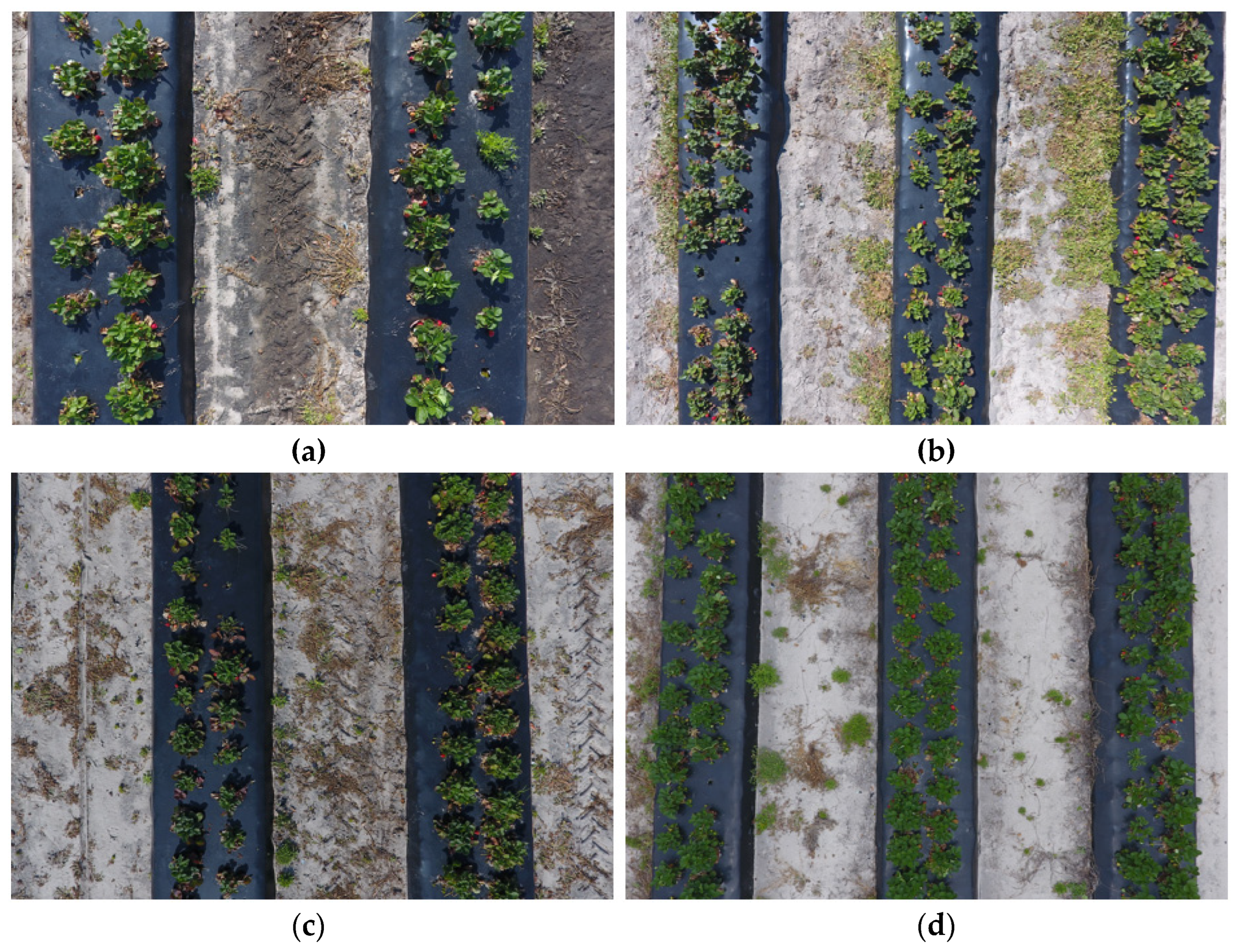
The drone collected data every 14 days and captured images 6 times in total. The shooting took place between 10:30 am and 12:30 pm, and the weather conditions were sunny and cloudy. Images under various weather conditions are used for model training to enhance its ability to recognize strawberry field images under different environmental conditions. The drone’s flight trajectory was parallel to the ridge and perpendicular to the top of the ridge, capturing images with a resolution of 4000 3000 pixels. When the drone captures images, the frontal overlap rate is 70% and the lateral overlap rate is 60%. All the flights were performed automatically by the DJI GroundStationPro (DJI Technology Co., Ltd., Shenzhen, China) iPad application, which is designed to conduct automated flight missions and manage the flight data of DJI drones. During each image capture, there are two flights conducted, capturing images from heights of 2 m and 3 m, respectively. The image capture at 2 m height takes 35 min per session, while the image capture at 3 m height takes 23 min per session. The initial images were divided into four types, and the example image is shown in Figure 1. The composition of the overall dataset is shown in Table 2. LabelImg 1.8.6 software was used to preprocess the original image, and the mature strawberries, immature strawberries, and strawberry flower targets were labeled, respectively. The annotated data was divided into a training set, a validation set, and a testing set in proportion. The final dataset composition is shown in Table 3.

Figure 1.
Drone dataset images captured under different conditions. (a) Sunny at a height of 2 m; (b) Sunny at a height of 3 mm; (c) Cloudy at a height of 2 m; (d) Cloudy at a height of 3 m.
Table 2.
Image acquisition information table.
Table 3.
Dataset information table.
2.2. The Improved YOLOv8 Model
The deep learning model proposed in this article is based on the network architecture of the YOLOv8 model and achieves rapid detection of targets in drone images by applying a slim–neck lightweight structure and shuffle attention module.
2.2.1. Shuffle Attention Module
Changes in flight altitude result in variations in the size of strawberry targets in captured images. The shuffle attention module utilizes channel attention and spatial attention calculations to extract feature maps of different scales. It was added to the backbone part of the original YOLOv8 model, and the feature mapping was divided into multiple groups to input into the shuffle attention module. Channel attention and spatial attention were calculated, respectively. All sub-features were aggregated to enhance feature extraction ability [21]. The specific structure of the shuffle attention module is shown in Figure 2.
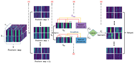
Figure 2.
Structure diagram of shuffle attention module. “c” represents the number of channels in the feature map, “h” represents the height of the feature map, and “w” represents the width of the feature map.
In step 1, feature maps of strawberry field images, , were input into the shuffle attention module, which were divided into g groups of feature maps along the depth direction, where was [, , …, ].
In step 2, for each group of feature maps , they were divided into and along two channel directions.
In step 3, was shrunk by the spatial dimension H W. Channel statistical information s was generated. s was further scaled and moved to ultimately generate channel attention . The specific calculation process of channel attention is shown in Equations (1) and (2).
where s represented channel information, H and W were feature map size, σϵ [0, 1], represented the parameter of channel information s for scaling and moving, and represented channel attention.
In step 4, was processed by GroupNorm and spatial statistical information y was generated. After linear transformation processing, the spatial attention was generated, and the specific calculation process of spatial attention is shown in Equations (3) and (4).
where represented the feature values of the c-th channel, i-th row, and j-th column in the feature map, was the mean of the g-th group, represented the variance of the g-th group, α was stability constant, was the parameter of transforming spatial information y, and was spatial attention.
In step 5, the channel Attention and the spatial attention were concatenated to generate the aggregated comprehensive attention . The sub-features obtained from different groups were shuffled and merged to obtain the final output of the module. The calculation process of the fused features is shown in Equations (5) and (6).
where represented comprehensive attention, g represented the number of original groups, and N was the number of groups after regrouping.
2.2.2. Slim–Neck Network
The GSConv module was introduced into the improve YOLOv8 model to reduce the complexity of calculation process of the traditional convolutional block CBL [22]. The specific structure of this module is shown in Figure 3.
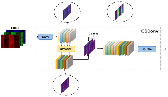
Figure 3.
The structure of the GSConv module.
The feature images of strawberry fields were subjected to regular convolution and down-sampling through the Conv module. The above results were deeply convolved through DWConv, and the output results of the two convolutions were concatenated and exchanged information through channel shuffle operation. The calculation process of ordinary convolution and deep convolution are shown in Equations (7) and (8).
where and represented the values of the i-th row, j-th column, k-channel. F and Fdw represented the kernel sizes of regular convolution and deep convolution, respectively. p and q represented the position of the convolution map on the feature map, m was the number of channels in the input feature map, S was the convolution step size, , , , and represented the weights and biases of regular convolution and deep convolution.
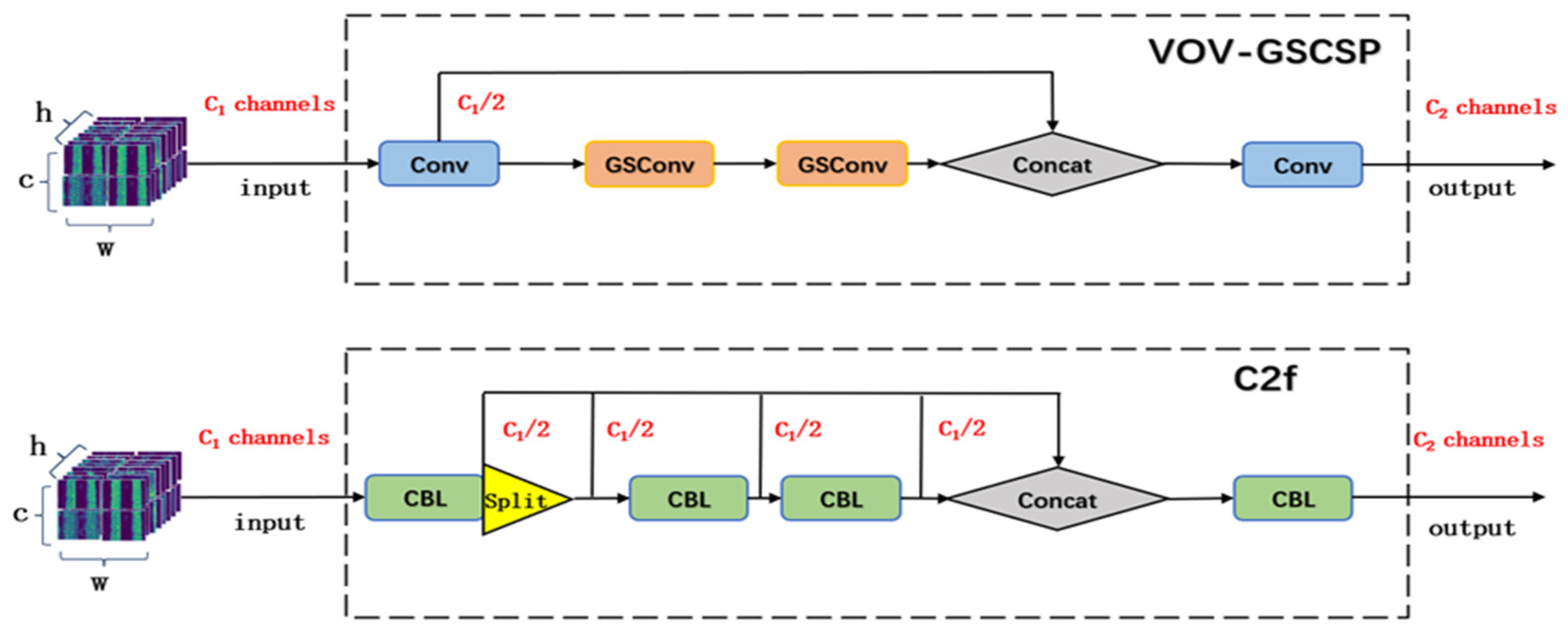
GSConv was used to build a lightweight VoV–GSCSP module, which replaced CBL blocks with lightweight convolutional GSConv based on the C2f module, and simplified the flow of channel information. Its detailed structure is shown in Figure 4. In the VOV–GSCSP module, channels of the input feature map were divided into two groups for processing. channels were processed by conv block convolution, and the other channels were processed by lightweight convolution of two additional GSConv modules. The processing results of the two parts were concatenated as the output of the module.
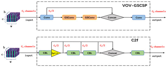
Figure 4.
The structure of the VOVGSCSP module.
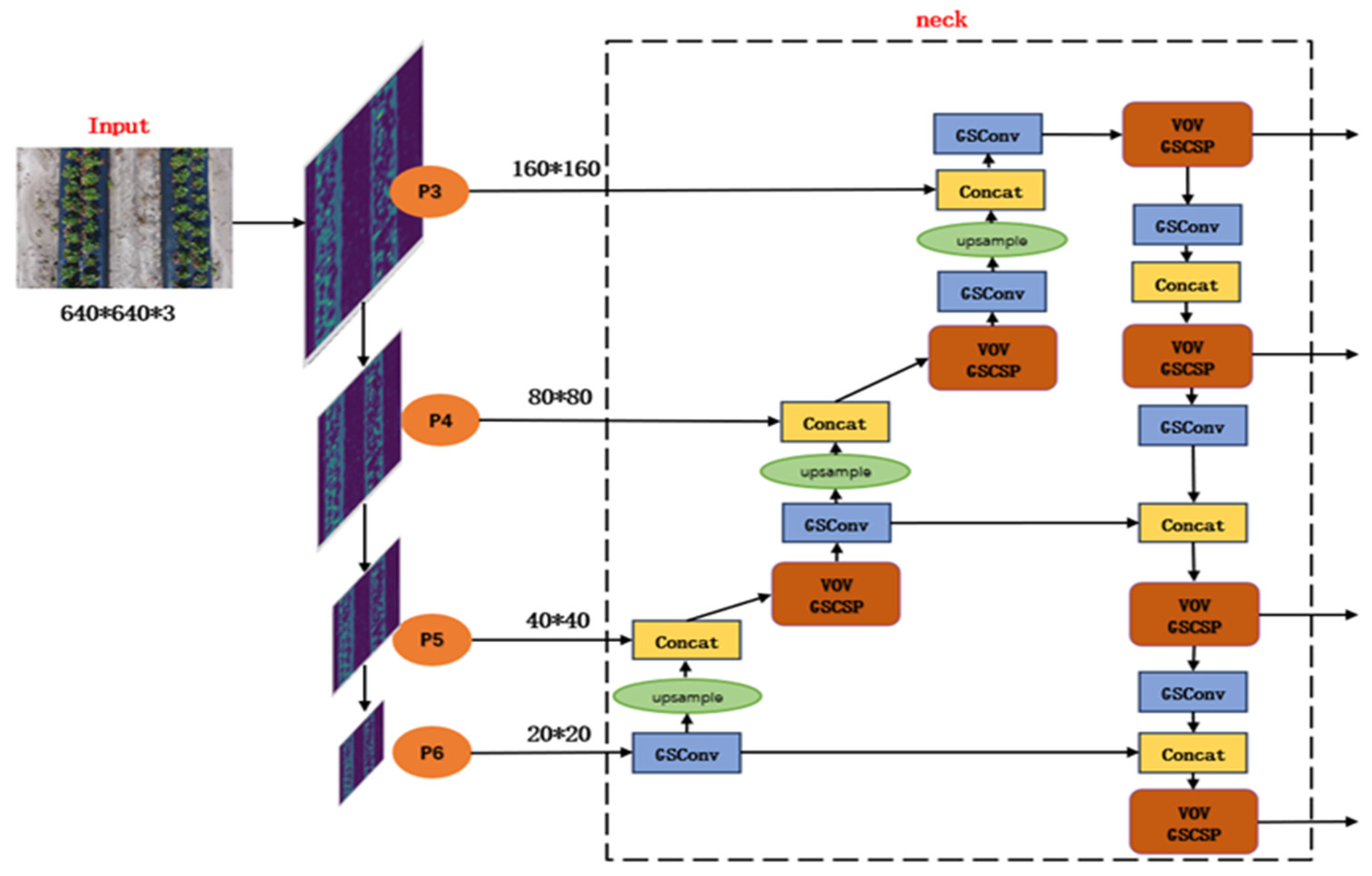
A small object detection layer added to the neck network was used to improve the resolution of the detection target, and the VoV–GSCSP module was used to reduce the size of the neck network. The neck network of the improved YOLOv8 model is shown in Figure 5. For example, a feature map with a resolution of 640 640 was input into the neck network. At the additional P3 detection layer, a feature map with a size of 160 160 was generated after two down-sampling operations with a step size of 2. More detailed feature information in this feature map could be used for small target detection.
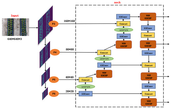
Figure 5.
Neck network of the improved YOLOv8 model.
2.3. Environmental Stability-Based Region Segmentation
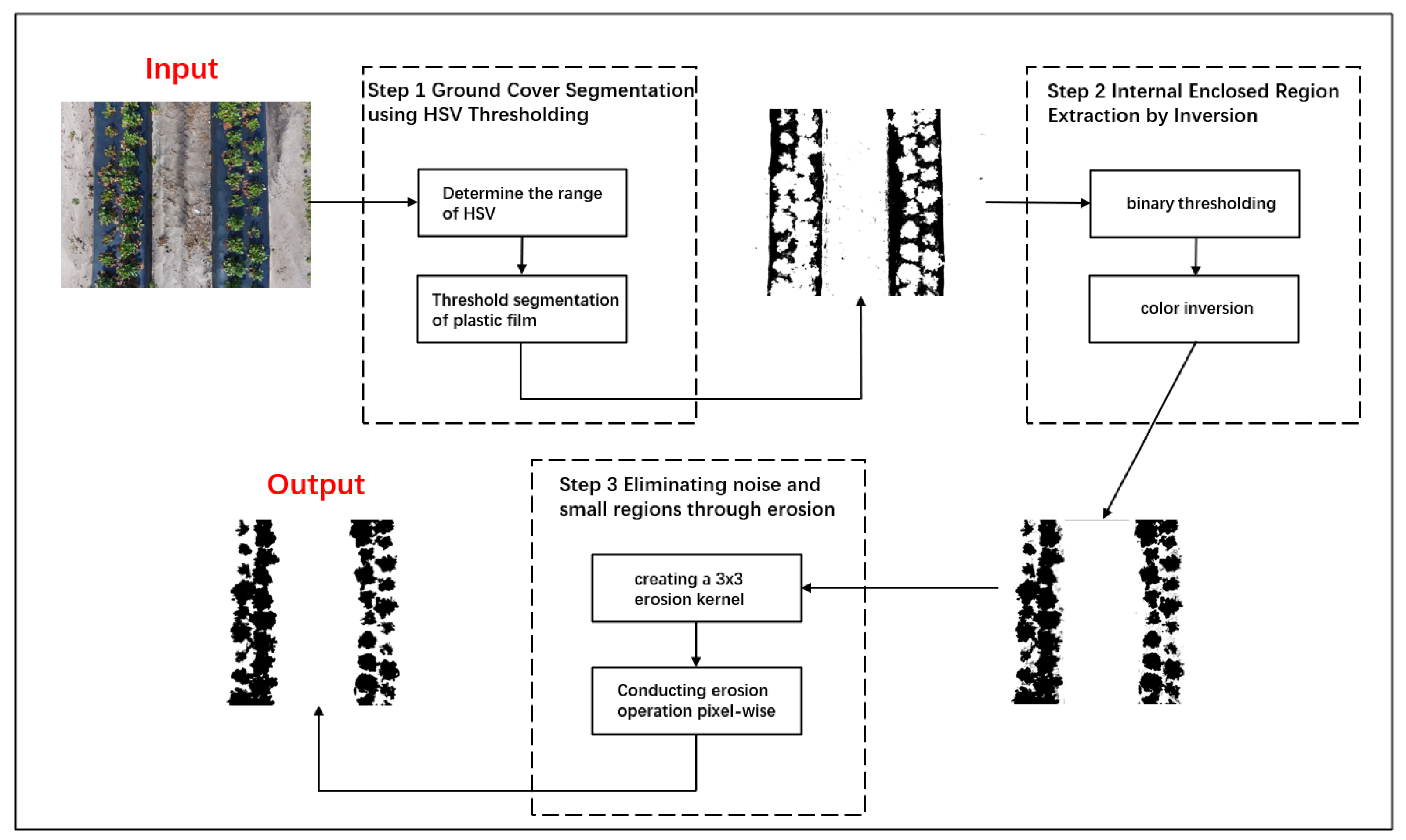
For the strawberry field images that have been detected by the improved YOLOv8 model, it is necessary to further combine the plant area and number to establish a subordinate relationship between the recognition target and the plant, which could be used to obtain the growth information of strawberries. In modern strawberry cultivation, plastic film is used to maintain soil temperature stability and reduce water loss [23]. Plastic film has a high absorption rate of ambient light and reflects less light, maintaining a relatively stable appearance in different environments [24]. This study indirectly obtained the strawberry plant area by segmenting the plastic film area with environmental stability. The segmentation process is shown in Figure 6.
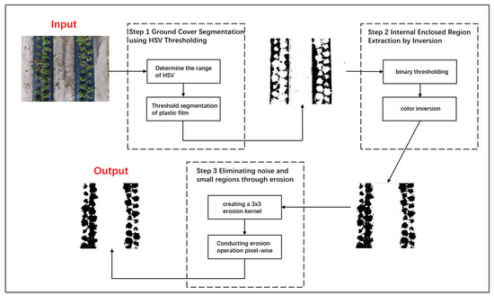
Figure 6.
The process of extracting plant areas.
In step 1, based on the color characteristics of black film, the threshold ranges of H, S, and V color channels were determined, ranging from 200 to 240, 30 to 70, and 10 to 60, respectively. Based on the above color range, the black plastic film area was accurately segmented.
In step 2, binarization processing was applied to images to achieve encoding of two different regions. Based on two different encoding methods, the color of the region was reversed.
In step 3, a corrosion core with a size of 3 3 was created, and the pixels in the image were traversed for corrosion operation. Noise and smaller areas were removed to complete the smoothness of the image. The calculation process of the corrosion operation is shown in Equation (9).
where S was that was the corrosion nucleus, represents the pixels after corrosion treatment, and i and j represented the element index of the corrosion nucleus.
2.4. Edge Extraction and Peak Detection Counting Method
2.4.1. Edge Extraction
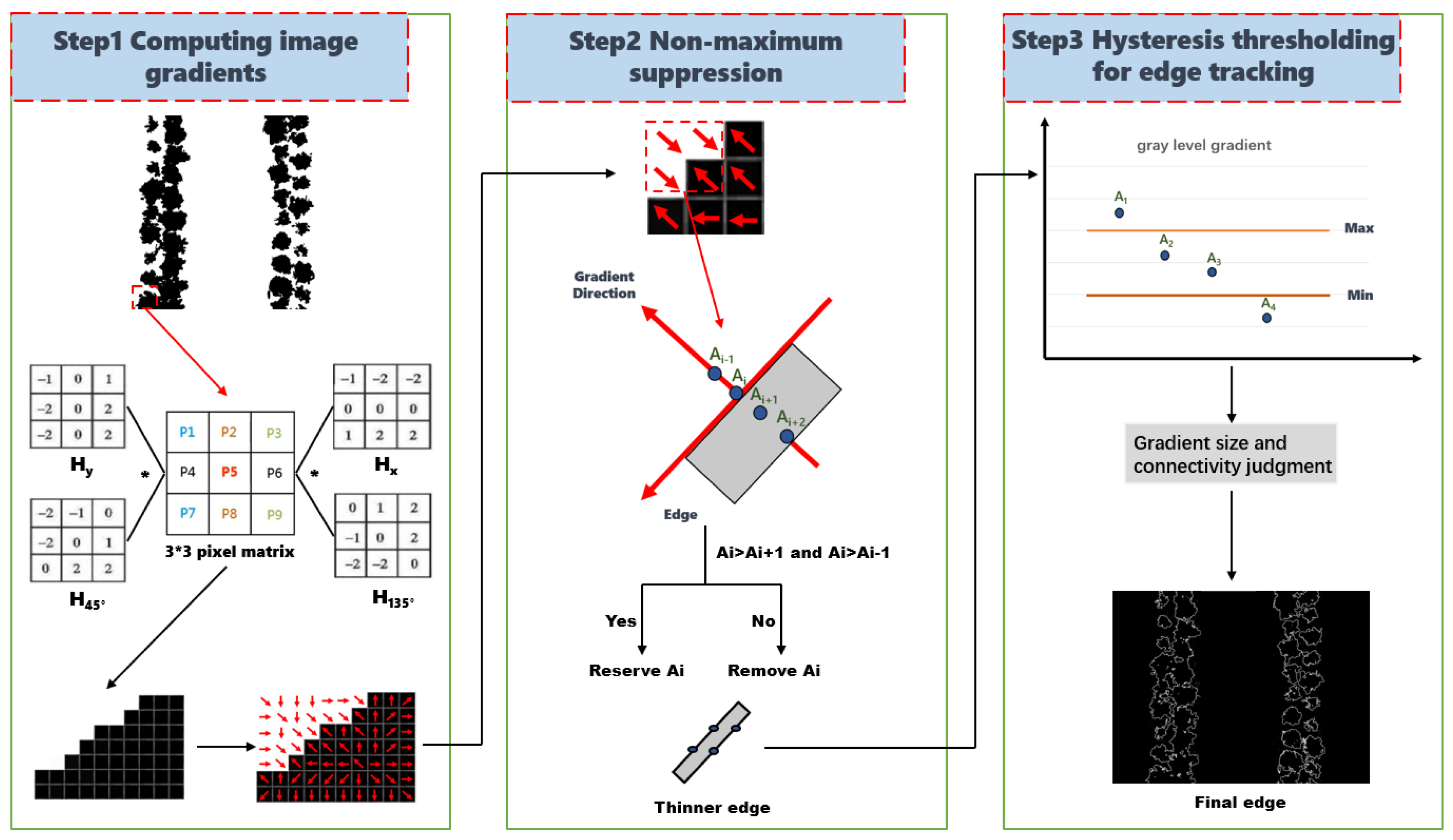
For the segmented plant area, the improved Diag–Canny edge detection algorithm was used to extract the boundary lines of the plant area, as shown in Figure 7.

Figure 7.
Edge extraction method process.
In step 1, for each pixel in the image, directional matrices and were added for expanding and refining gradient direction based on directional matrices and of the classical Canny algorithm. The specific calculation process is shown in Equations (10) and (11).
where i and j represented pixel coordinates, , , , and represented different directional matrices, M [i, j] was gradient amplitude, and D [i, j] was gradient direction.
In step 2, all points on the gradient matrix were traversed, and their gradient directions were approximated as eight directions (horizontal and vertical directions, and expand in the 45 degree and 135 degree directions). Gradient intensity of pixels and in the positive and negative directions of gradients were compared. If the gradient intensity of was maximum, it was retained, and if otherwise it was suppressed. The specific calculation process is shown in Equation (12).
where represented the result of pixel processing, and M[i − 1,j] and M[i + 1,j] represented the gradient intensity of pixels in the positive and negative directions of their gradients.
In step 3, an edge detection method based on dual thresholds was used to refine the edge curve. The maximum and minimum gradient thresholds, Max and Min, were set. If the gradient intensity of a pixel was greater than Max, the pixel was confirmed as an edge point. If the gradient intensity of a pixel was between Max and Min, and was connected to the edge point, it was determined as the edge point. Otherwise, they would be judged as non-edge points. After the above processing, the final edge of the plant area was obtained.
2.4.2. Peak Detection
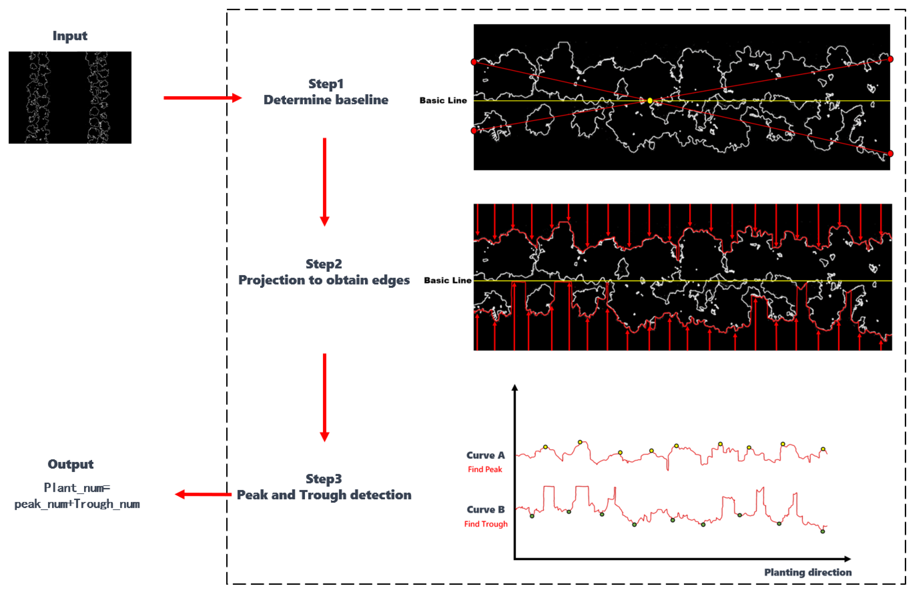
The changes in the edge lines on both sides of the continuous plant area were obtained by using the projection method. The peak and valley detection algorithm was used to estimate the number of strawberry plants. The specific processing flow is shown in Figure 8.
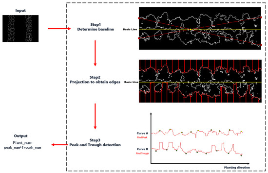
Figure 8.
Peak detection method process.
In step 1, the diagonal lines of the edge points on both sides of the area were connected, and the horizontal basic line through their intersection points was drawn.
In step 2, the edge curves were obtained from the intersection points projecting from vertically downwards and vertically upwards. If the projection line did not intersect with the edge curve, the intersection point with the basic line was taken as the result, and the changes in the edge lines on both sides of the plant area were obtained.
In step 3, the peak detection algorithm and valley detection algorithm were used respectively to detect the upper edge curve A and the lower edge curve B. The number of regional plants was the sum of the number of peaks and valleys.
2.5. Growth Information Map
The improved YOLOv8 network was used to recognize the quantity and position information of strawberries at different stages. The image is processed by ground segmentation using HSV thresholding, internal enclosed region extraction by inversion, and eliminating noise to obtain the strawberry plant area. The peak detection was used to calculate plant quantity information. The overall growth map of the strawberry field was drawn. The conversion relationship between actual distance and pixel distance could be calculated using GSD (ground sample distance). The specific calculation process is shown in Equation (13).
where λ represented the pixel size of the camera sensor, H represented the image shooting height, and c represented the camera focal length.
As shown in Figure 9, strawberry flowers usually took 21–30 days to grow into complete fruit, while immature strawberries usually took 7–14 days to fully mature [25]. If mature strawberries were not picked after maturity, they would begin to rot after 1–3 days. Weights were set based on the number of mature strawberries, immature strawberries, and strawberry flowers over time. The numbers of different plant objects were summed up, and divided by the number of strawberry plants. The result was defined as a strawberry growth parameter α. The size of this parameter could reflect the maturity of the region and the priority of picking. Based on the size of this parameter, different colors were used to draw regional growth maps, including strawberry growth parameters α. The calculation process is shown in Equation (14).
where , , and represented the number of mature strawberries, immature strawberries, and strawberry flowers, respectively.
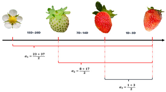
Figure 9.
Changes in strawberry growth stage.
The method for obtaining the growth information map of strawberry fields is shown in Figure 10. The drone ran along the preset path and obtained images of different parts of the strawberry field area. The regional image was input into the improved YOLOv8 network, and strawberry targets at different growth stages were recognized. The environmental stability-based segmentation was used to extract the strawberry plant area (including fruits, stems, and leaves). Edge extraction and peak detection was used to estimate the number of strawberry plants. Based on the number of strawberry plants and the distribution of mature strawberries, we drew a growth chart of strawberries (reflecting the urgency of picking in different regions). The growth maps of strawberry fields in different regions were concatenated according to the shooting path order, and the overall growth map of the strawberry field was obtained.
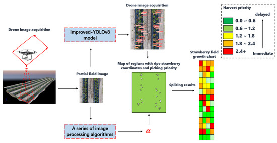
Figure 10.
Flow chart of drawing strawberry growth information map.
2.6. Experiment
To validate the effectiveness of the proposed model and image-processing algorithm in this study, four sets of experiments were conducted sequentially.
In the first set of experiments, the improved YOLOv8 model proposed in this study, along with several common deep learning network models, such as models of YOLOv3, YOLOv4, YOLOv5n, YOLOv7, YOLOX, YOLOv8n, SSD-vgg16, and Faster R-CNN, was trained using the same dataset. A comparative performance analysis of the models was conducted. The hardware environment of the experiment was mainly a computer equipped with an Intel i5-13600kf processor, 32 GB RAM, and GeForce GTX 4080 GPU. The computer used CUDA 11.2 parallel computing architecture and NVIDIA cuDNN 8.0.5 GPU acceleration library. The software simulation environment was the Pytorch deep learning framework (Python version 3.10). Anaconda was used to configure and manage the virtual environment, and Pycharm was used to compile and run programs. Model performance metrics mainly included P (precision), R (recall), F1 (harmonic average), AP (average precision), mAP@0.5 (mean average precision), as shown in Equations (15)–(19).
where represents the number of strawberries correctly identified, represents the number of strawberries incorrectly identified, represents the number of missed strawberries, represents the total number of images, and represents the number of categories of the strawberry maturities. represents that the integral of accuracy rate to recall rate is equal to the area under the P–R curve, and is the average of the average precision of all categories.
The second set of experiments was used to segment plant areas using the proposed environment stability-based region segmentation method, based on different color spaces of RGB, HSV, and Lab, in order to find the best color space type suitable for threshold segmentation. The overlap between the proposed method and the actual manually calibrated area was compared and analyzed to determine the optimal color space suitable for this algorithm, and the segmentation effect of the proposed algorithm was tested.
In the third set of experiments, edge extraction and peak detection algorithms were used to process the segmented strawberry plant area, estimate the number of plants in the area, and compare it with the actual number of plants. A total of fifty drone images taken from a height of 2 m were located in the first group, and fifty drone images taken from a height of 3 m were located in the second group. Errors were recorded and analyzed.
In the fourth set of experiments, the regional growth map was drawn. According to the actual geographic information and shooting sequence captured by the drone, all regional growth maps were concatenated, and the overall strawberry growth map of the farmland was drawn. The picking priority information of the growth map was observed and analyzed. A total of ten strawberry cultivation experts assigned picking priorities to different areas of the entire strawberry field based on their experience (a total of 5 levels). A comparative analysis was conducted between these priorities and the growth charts generated in this study.
3. Results
3.1. Performance and Comparison of the Proposed Model
The performance parameters, precision, recall, and F1 score of the improved YOLOv8 model and other models under the input conditions of img_size 640 and img_size 1280 are shown in Table 4. The recognition results of the proposed model are shown in Figure 11.
Table 4.
Comparison of the results of different models.
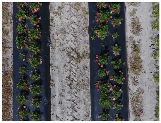
Figure 11.
Detection results of the proposed model.
For all the models used in the experiment, when img_size was 1280, there was a significant improvement in precision, recall, and F1score, compared to what was obtained when img_size was 640. The average precision, recall, and F1score had increased. Compared with the parameters between different models, the precision of the improved YOLOv8 model was 93.4, which was higher than those of other models. Its recall was 94, higher than those of most models but, however, 3 lower than the 97 of the YOLOv7 model. The F1score value of the proposed model was 93.69, which was 25.42, 35.59, 12.05, 8.16, 18.45, 5.91, 32.36, and 8.65 higher than those of other models, respectively. For the detection results shown in Figure 11, the improved YOLOv8 model could accurately detect and distinguish strawberry targets at different growth stages in the image.
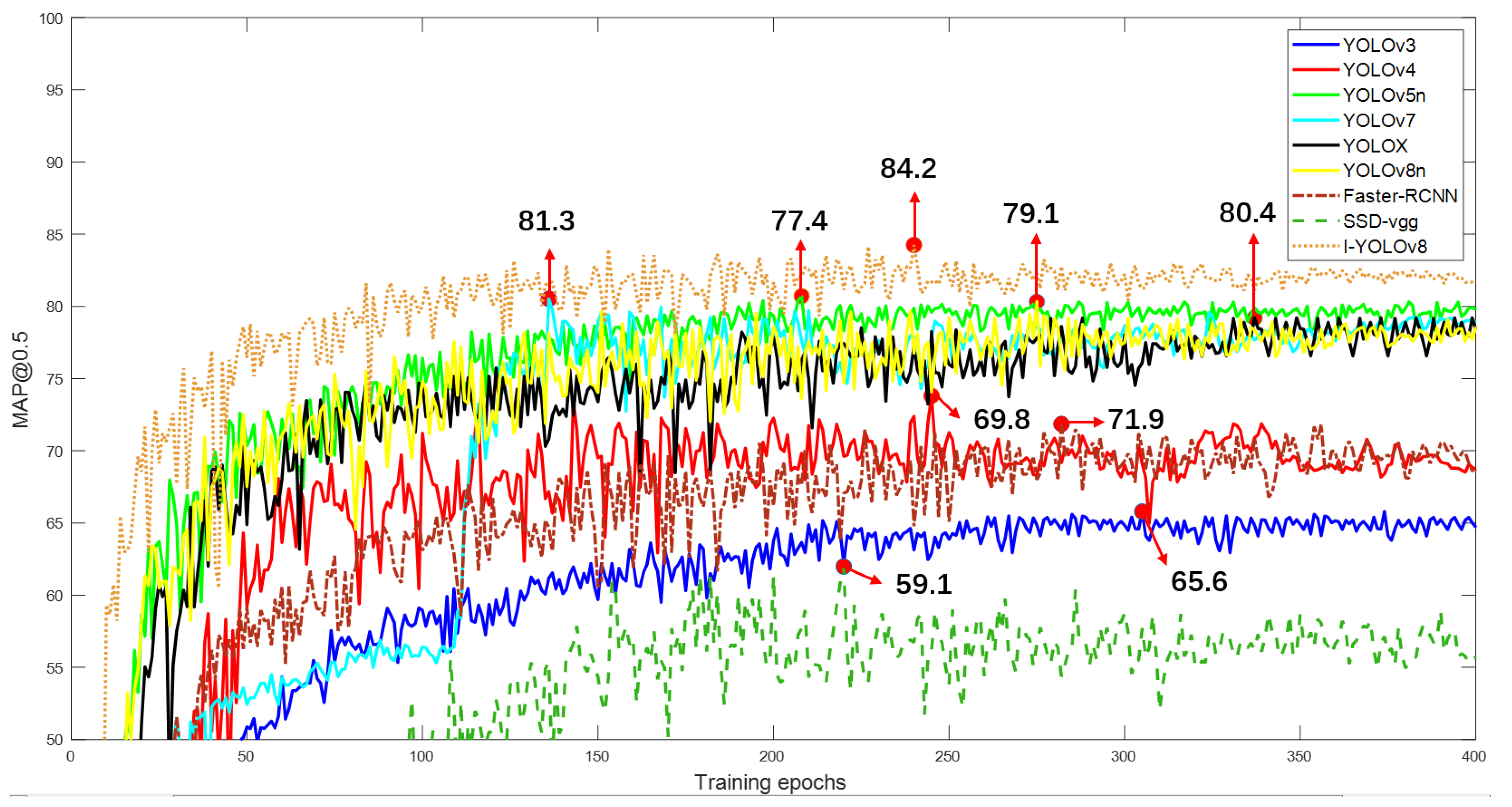
The map@0.5 value change of the improved YOLOv8 model compared to other models during the training process is shown in Figure 12.
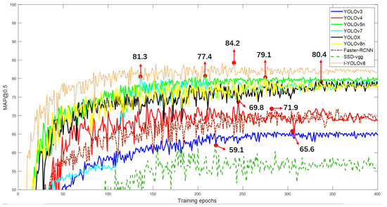
Figure 12.
The map@0.5 value change curves of different models.
The red dots represent the positions with the highest map@0.5 values on each curve, and the red arrows connect the points with their map@0.5 values. The map@0.5 value of the proposed model gradually increased during the training and stabilized after reaching 200 epochs. Compared to the SSD–vgg curve, the improved YOLOv8 curve and the YOLOv5n curve exhibited a more stable upward trend. The optimal map@0.5 value of the proposed model was 84.2, which was 18.6, 14.4, 6.8, 2.9, 3.7, 5.1, 12.3, and 25.1 higher than those of the models of YOLOv3, YOLOv4, YOLOv5n, YOLOX, YOLOv8n, Faster R-CNN, and SSD-vgg16, respectively.
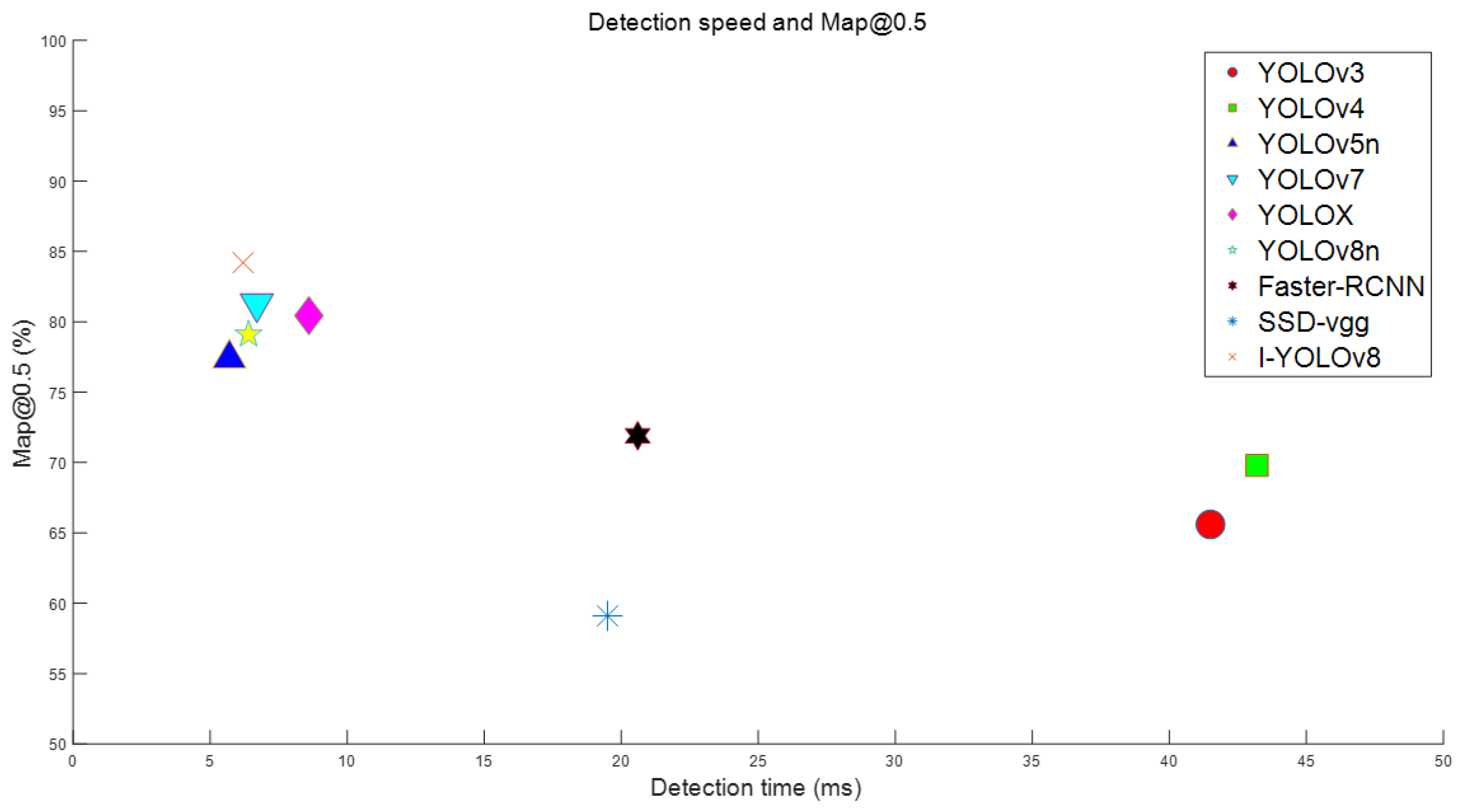
The scatter plot between the detection speed and accuracy of different models is shown in Figure 13. The detection speed of the improved YOLOv8 model was 6.2 ms, slightly higher than the YOLOv5n model’s 5.7 ms, but, however, faster than other models. The improved YOLOv8 model had the highest map@0.5 value. The detection speed could indirectly reflect the size of the model. The proposed model used the VOV–GSCSP module to optimize the C2f module in the neck part of the traditional YOLOv8 model. The module simplified the complexity of convolution operations and reduced model volume, while maintaining a high degree of accuracy.
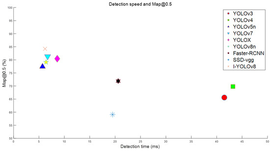
Figure 13.
Scatter plot of different models between detection speed and accuracy.
3.2. Results Based on Threshold Segmentation
The results of segmenting 10 images taken from different environments and different color spaces, as well as the effective segmentation area data, are shown in Table 5. The segmentation results of four images are shown in Figure 14. According to Table 5, the segmentation accuracy of HSV-based threshold segmentation on different images was relatively stable, with an average segmentation accuracy of 86.12%, which was 7.91% higher than the result from RGB-based threshold segmentation, and 10.01% higher than the result from LAB-based threshold segmentation, respectively. In Figure 14, it can be seen that the threshold segmentation based on HSV accurately segmented the plastic film area, which was close to the manually calibrated area range. The threshold segmentation based on RGB did not have clear boundaries in the internal area of the plastic film, making it difficult to accurately segment the internal contours. While the threshold segmentation based on LAB could accurately segment the internal contour of the plastic film there were, however, many noise points in the image.
Table 5.
Segmentation results based on different color spaces.
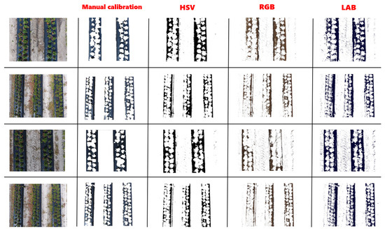
Figure 14.
Segmentation results in images based on different color spaces.
3.3. Counting Results
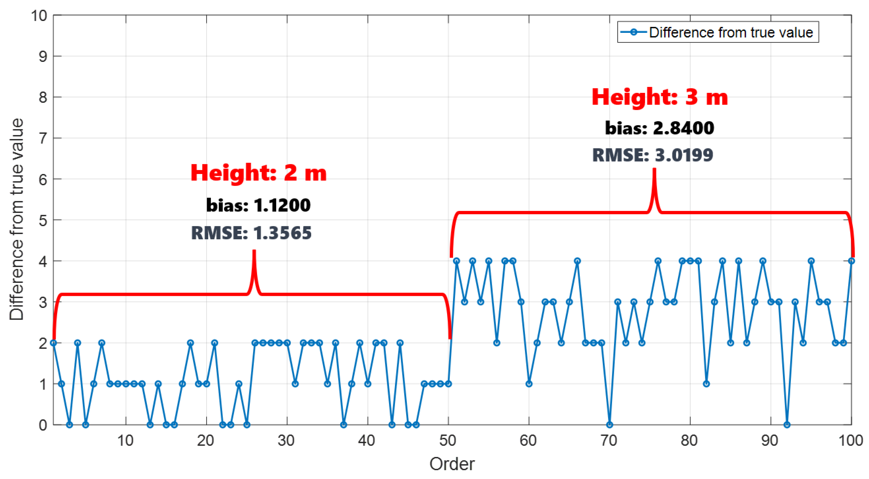
In being combined with the results of plant region segmentation, the number of plants in the region was estimated using edge extraction and peak detection methods. The errors between the estimated number and actual manual counting results are shown in Figure 15.
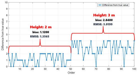
Figure 15.
The errors between the estimated number and actual manual counting results.
The bias of the error for the first set of images captured at a height of 2 m is 1.1200, and the rmse is 1.3565; The bias of the error for the second set of images captured at a height of 3 m is 2.8400, and the rmse is 3.0199; In the 100 images tested in the experiment, the estimated number of plants was generally lower than the actual number of plants.
3.4. Results of Growth Information Map
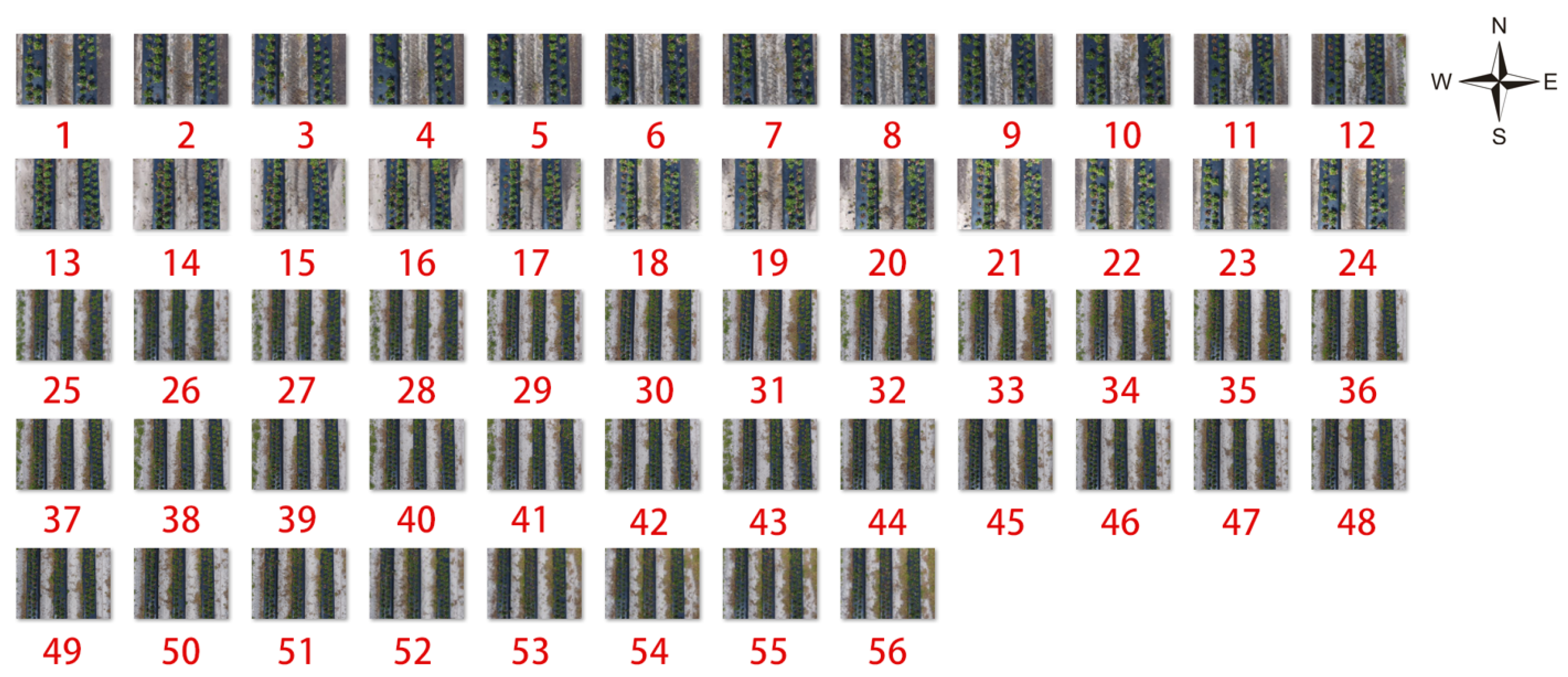
The drone traversed the entire orchard and captured images of 56 areas, as shown in Figure 16. The method proposed in this study was used to obtain the 56 regional growth information maps. The growth information maps were concatenated according to the original image position to obtain the growth information map of the overall strawberry field, as shown in Figure 17. The conformity between the region picking priorities derived from the overall growth chart in this study and those provided by 10 experts is shown in Table 6. The growth status information of strawberries in different regions is shown in Figure 18 and Table 7.

Figure 16.
56 regions of the overall strawberry field.

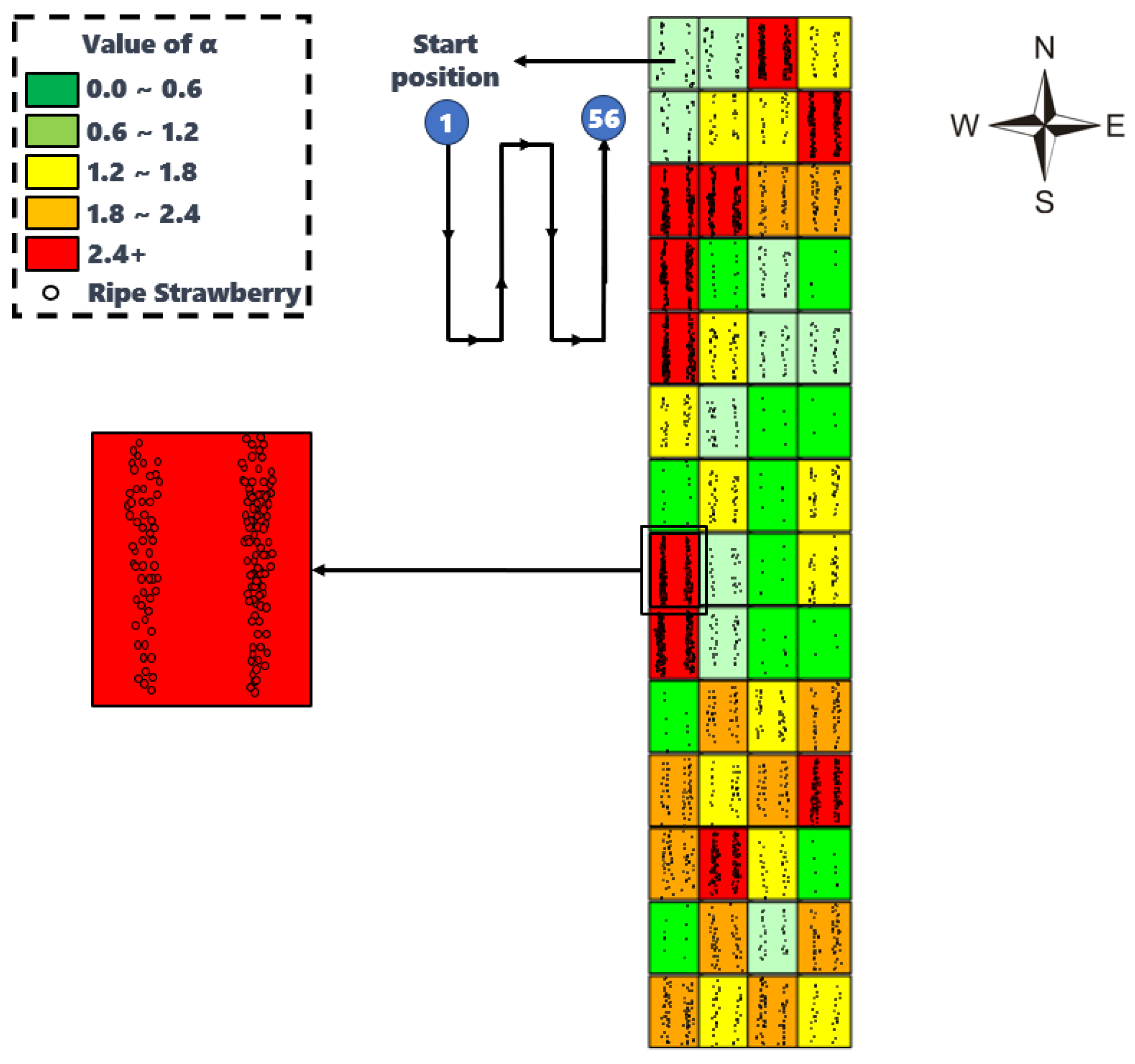
Figure 17.
The growth information map of the overall strawberry field.
Table 6.
The alignment between the picking priorities in this study and those given by experts.
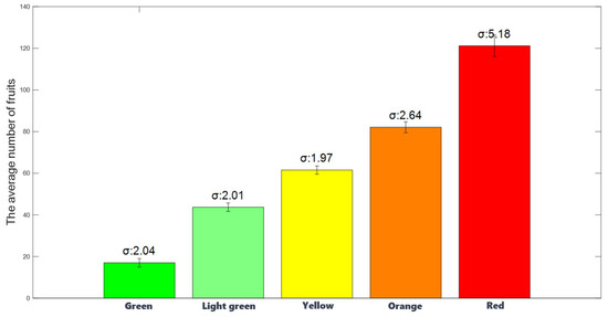
Figure 18.
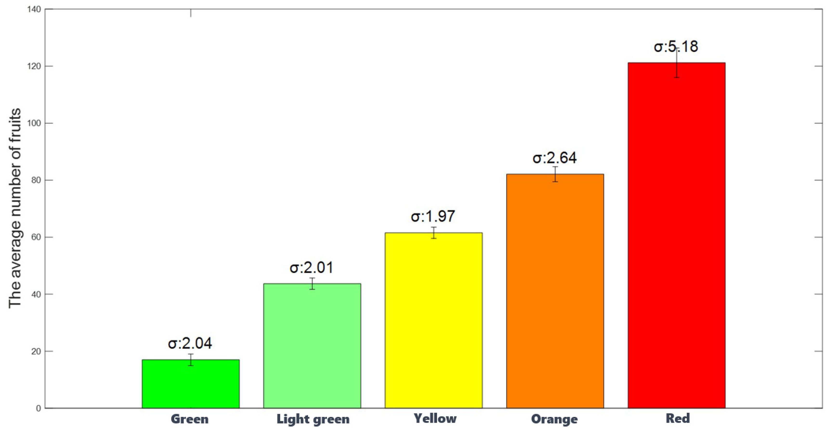
Number of strawberry fruits with different representative colors.
Table 7.
Information on the growth status in different areas of the strawberry field.
In Figure 17, the red area accounts for 17.8% of the total area. This type of area has more mature strawberries, and many strawberries will be mature in the future. Harvesting work should be carried out as soon as possible to reduce the decay of strawberry fruits in these areas. The green area accounts for 39.3% of the total area, and the number of mature strawberries in this type of area was relatively small compared to the number of strawberries that would mature soon, resulting in a lower priority for harvesting. The orange–yellow area accounts for 42.9% of the total area, and this type of area had a moderate number of mature strawberries, and there would also be a certain number of strawberries maturing in the future. Attention should be paid to these areas and a later harvest plan should be formulated. From the perspective of regional distribution, the maturity of strawberries in the southern part of the farmland was faster than that in the northern part, and the maturity of strawberries in the eastern and western parts was faster than that in the central part. The assessment of picking priorities for various regions of the strawberry field in this study yielded an average accuracy of 80.53%, based on those provided by 10 experts. This accuracy ensures precise guidance for harvesting.
According to Table 7, the values of “Ratio of the total fruit count to the plant size” can reflect the maturity status in different areas. In the regions represented by green color, the minimum ratio is 2.71, and the maximum is 10.95. In the regions represented by light green color, the minimum ratio is 14.34, and the maximum is 20.77. In the regions represented by yellow color, the minimum ratio is 21.07, and the maximum is 28.13. In the regions represented by orange color, the minimum ratio is 28.90, and the maximum is 39.75. In the regions represented by red color, the minimum ratio is 41.97, and the maximum is 61.57. For areas with a larger number of strawberries ready for harvest or smaller strawberry plant areas, their harvest index is higher. Conversely, for areas with fewer strawberries ready for harvest or larger strawberry plant areas, their harvest index is lower. The different colors set in this study correspond to the range of changes in the harvest index. According to Figure 18, the average number of strawberry fruits representing colors green, light green, yellow, orange, and red, are 17.00, 43.70, 61.54, 82.10, and 121.2, respectively, showing an increasing trend in fruit quantity. The standard deviations within groups of different representative colors are 2.04, 2.01, 1.97, 2.64, and 5.18, respectively, indicating smaller variations within groups of the same representative color. The one-way ANOVA analysis conducted on the fruit quantity data for different colors yielded an F-ratio of 5.3067, which is less than 265.783 (α = 0.001), indicating a significant association between the representative color of the fruit and the quantity of fruits.
4. Discussion
The drone image has the characteristics of high resolution, wide coverage, and multiple and small targets to be identified. The improved YOLOv8 model added two additional small object detection layers and set the img_size of the input image to 1280. During the training process, the size of the target feature map was enlarged, which was beneficial for the model to learn target features. Adding a detection layer of small targets could improve the detection effect on small targets, and similar conclusions could be found in the article [26]. The precision and recall of the proposed model have significantly improved, which reflects the proposed model had high detection accuracy.
The performance curve of the proposed model showed little fluctuation during the training process, which indicated that the model could effectively learn strawberry features at different stages and the training was efficient. This accounted for the advantages of the shuffle attention module application, which effectively learned the relationship between different channel information at the same position of the strawberry target, as well as the spatial information between different positions. The module enabled the target features to be effectively obtained by the proposed model, while also distinguishing the differences in features between different positions, improving the detection accuracy of the model and enhancing its stability and robustness. The shuffle attention module could improve the learning performance of the model, and similar conclusions can be found in the article [27].
The VOV–GSCSP module could reduce network complexity and maintain certain accuracy in small object detection, and a similar conclusion can be found in the article [28]. The additional small object detection layer brought about an increase in model volume, which could be optimized through the VOV–GSCSP module, giving the proposed model advantages such as small model volume, high recognition accuracy, and fast detection speed. It could be effectively applied to the recognition of strawberry targets at different growth stages in drone images.
The target of segmentation was the black plastic film area, which had stable color in different environments and was easy to segment. Therefore, the method of obtaining the plant area through the plastic film area was accurate and efficient. The RGB color space mixed lighting components into three color channels. For area segmentation in drone images with lighting changes, the boundaries of the segmented areas were unclear and could not be further applied to plant area segmentation. While the Lab color space considered lighting as a separate component, it however had the characteristic of uniform perception. The color changes at equal intervals are the same, making it difficult to effectively distinguish between noise and target areas, resulting in more noise in the segmentation results. Based on the segmentation of HSV color space, while considering lighting separately, the noise was eliminated by integrating changes in hue and saturation, accurately segmenting black film areas in different environments. HSV color space-based segmentation could be adapted to lighting and reduce noise. A similar conclusion can be found in the article [29].
Based on the proposed method of combining edge extraction and peak detection, the number of strawberry plants in drone images was estimated. The calculated values were generally lower than the actual values, and the reason may be that during the peak detection process, the curve amplitude of some continuous plants changed similarly, and multiple peaks were detected as one peak, introducing errors. However, this method could generally accurately count the number of plants in a region and, the smaller the area, the better the detection effect.
By observing the overall growth information map of the strawberry field, harvesting plans could be formulated based on the picking priority in different regions. During the irregular batch ripening period of strawberries, labor distribution could be reasonably planned to ensure high-quality harvesting of strawberries and reduce the economic losses caused by strawberry decay. Compared to manually evaluating picking priorities, the overall growth chart can also view the distribution of different picking priorities and guide the path planning of the harvesting robot [30].
Based on the observations from Table 7 and Figure 18, the method proposed in this study not only calculates regional ripeness but also assesses the size and productivity of strawberry plants. During plant growth, as the allocation of dry matter increases towards leaves and runners, an increase in plant volume decreases the harvest index. When plant volume reaches a certain threshold, strawberry plant yield decreases [31]. The method proposed in this study suggests that smaller plants are indeed more productive. Farmers can adjust nitrogen fertilizer dosage to control plant size, thus enabling plants to have a higher harvest index and increase overall yield.
5. Conclusions
This study proposed a lightweight deep learning model based on YOLOv8n improvement, which accurately identified strawberries at different growth stages in drone images. A region segmentation algorithm based on environmental stability was proposed to effectively segment the strawberry plant region. A plant counting method based on edge extraction and peak and valley detection was proposed to estimate regional plant numbers. Based on the above methods, a growth information map was created to visualize the growth situation of different areas of strawberry fields and assist farmers in formulating harvesting plans. The main conclusions are as follows.
- An improved YOLOv8 model was constructed by replacing the neck network of the YOLOv8n model with the VOV–GSCSP block, applying the shuffle attention block, and adding two small object detection layers.
- The Improved YOLOv8 model demonstrated an average accuracy of 82.5% in identifying immature strawberries, 87.4% for mature ones, and 82.9% for strawberry flowers in drone images. The model’s performance metrics included a mean average precision (mAP) of 84.2%, precision (P) of 93.4%, recall of 94%, and an F1 score of 93.69%. Additionally, the model exhibited an average detection speed of 6.2 ms and had a compact model size of 20.1 MB.
- The region segmentation algorithm based on environmental stability showed performance in which the average proportion of the segmentation area to the actual area was 86.12% for the plastic film area surrounding the plant.
- The proposed method for estimating the number of plants by combining edge extraction and peak detection had a counting error within 1 in drone images at a height of 2 m, and within 3 in drone images at a height of 3 m.
- The created growth information map of the strawberry field could provide intuitive information on the recent maturity of strawberries in different regions and assist farmers in determining the harvesting priorities in different areas during peak picking periods; it would also help them when developing harvesting plans, and would drive improvements in the quality of harvested strawberries.
These conclusions confirmed that the proposed model with the image-processing technology had effective performance for detecting strawberry objects in drone images and creating the growth information map of strawberries. Future research will capture continuous images of strawberry plants throughout their growth stages, utilize the method proposed in this study to quantify harvest indices, and combine them with the nutritional status of the plants for analysis, providing valuable insights for farmers.
Author Contributions
Conceptualization, C.W., Q.H. and C.L.; methodology, C.W., F.W. and J.L.; investigation, Q.H., D.K. and C.L.; resources, C.W., F.W. and X.Z.; writing—original draft preparation, Q.H.; writing—review and editing, C.W. and Q.H.; project administration, J.L. and D.K.; funding acquisition, C.W. All authors have read and agreed to the published version of the manuscript.
Funding
This work was supported by grants from the National Natural Science Foundation of China (52005069), the Guangdong Basic and Applied Basic Research Foundation (2022A1515140162), the Yunnan Major Science and Technology Special Plan (202302AE090024), and the Yunnan Fundamental Research Projects (202101AT070113).
Institutional Review Board Statement
Not applicable.
Informed Consent Statement
Not applicable.
Data Availability Statement
The data presented in this study are openly available at https://github.com/abysswatcher-hqy/I-YOLOv8-model (accessed on 1 January 2020).
Conflicts of Interest
We declare that we do not have any commercial or associative interests that could be viewed as representing a conflict of interest in the work submitted.
References
- Lin, Y.; Liang, W.; Cao, S.; Tang, R.; Mao, Z.; Lan, G.; Zhou, S.; Zhang, Y.; Li, M.; Wang, Y.; et al. Postharvest Application of Sodium Selenite Maintains Fruit Quality and Improves the Gray Mold Resistance of Strawberry. Agronomy 2023, 13, 1689. [Google Scholar] [CrossRef]
- Chen, J.; Mao, L.; Mi, H.; Zhao, Y.; Ying, T.; Luo, Z. Detachment-accelerated ripening and senescence of strawberry (Fragaria x ananassa Duch. cv. Akihime) fruit and the regulation role of multiple phytohormones. Acta Physiol. Plant. 2014, 36, 2441–2451. [Google Scholar]
- Ono, S.; Yasutake, D.; Kimura, K.; Kengo, I.; Teruya, Y.; Hidaka, K.; Yokoyama, G.; Hirota, T.; Kitano, M.; Okayasu, T.; et al. Effect of microclimate and photosynthesis on strawberry reproductive growth in a greenhouse: Using cumulative leaf photosynthesis as an index to predict the time of harvest. J. Hortic. Sci. Biotechnol. 2023, 99, 223–232. [Google Scholar] [CrossRef]
- Van, B.; Vandendriessche, T.; Hertog, M.; Nicolai, B.; Geeraerd, A. Detached ripening of non-climacteric strawberry impairs aroma profile and fruit quality. Postharvest Biol. Technol. 2014, 95, 70–80. [Google Scholar]
- Metwaly, E.; AL-Huqail, A.; Farouk, S.; Omar, G. Effect of Chitosan and Micro-Carbon-Based Phosphorus Fertilizer on Strawberry Growth and Productivity. Horticulturae 2023, 9, 368. [Google Scholar] [CrossRef]
- Liu, J.; Zhao, S.; Li, N.; Faheem, M.; Zhou, T.; Cai, W.; Zhao, M.; Zhu, X.; Li, P. Development and Field Test of an Autonomous Strawberry Plug Seeding Transplanter for Use in Elevated Cultivation. Appl. Eng. Agric. 2019, 35, 1067–1078. [Google Scholar] [CrossRef]
- Tang, Y.; Qi, S.; Zhu, L.; Zhuo, X.; Zhang, Y.; Meng, F. Obstacle Avoidance Motion in Mobile Robotics. J. Syst. Simul. 2023, 36, 1. [Google Scholar]
- Meng, F.; Li, J.; Zhang, Y.; Qi, S.; Tang, Y. Transforming unmanned pineapple picking with spatio-temporal convolutional neural networks. Comput. Electron. Agric. 2023, 214, 108298. [Google Scholar] [CrossRef]
- Chen, M.; Chen, Z.; Luo, L.; Tang, Y.; Cheng, J.; Wei, H.; Wang, J. Dynamic visual servo control methods for continuous operation of a fruit harvesting robot working throughout an orchard. Comput. Electron. Agric. 2024, 219, 108774. [Google Scholar] [CrossRef]
- Bian, C.; Shi, H.; Wu, S.; Zhang, K.; Wei, M.; Zhao, Y.; Sun, Y.; Zhuang, H.; Zhang, X.; Chen, S. Prediction of Field-Scale Wheat Yield Using Machine Learning Method and Multi-Spectral UAV Data. Remote Sens. 2022, 14, 1474. [Google Scholar] [CrossRef]
- Feng, Q.; Shao, Z.; Wang, Z. Boundary-aware small object detection with attention and interaction. Vis. Comput. 2023, 1–14. [Google Scholar] [CrossRef]
- Feng, F.; Gao, M.; Liu, R.; Yao, S.; Yang, G. A deep learning framework for crop mapping with reconstructed Sentinel-2 time series images. Comput. Electron. Agric. 2023, 213, 108227. [Google Scholar] [CrossRef]
- Wang, Y.; Yan, G.; Meng, Q.; Yao, T.; Han, J.; Zhang, B. DSE-YOLO: Detail semantics enhancement YOLO for multi-stage strawberry detection. Comput. Electron. Agric. 2022, 198, 107057. [Google Scholar] [CrossRef]
- Li, J.; Zhu, Z.; Liu, H.; Su, Y.; Deng, L. Strawberry R-CNN: Recognition and counting model of strawberry based on improved faster R-CNN. Ecol. Inform. 2023, 77, 102210. [Google Scholar] [CrossRef]
- Du, X.; Cheng, H.; Ma, Z.; Lu, W.; Wang, M.; Meng, Z.; Jiang, C. DSW-YOLO: A detection method for ground-planted strawberry fruits under different occlusion levels. Comput. Electron. Agric. 2023, 214, 108304. [Google Scholar] [CrossRef]
- Yoon, S.; Jung, S.; Steven, B.; Ha, S.; Sung, K.; Dong, S. Prediction of strawberry yield based on receptacle detection and Bayesian inference. Heliyon 2023, 9, e14546. [Google Scholar] [CrossRef] [PubMed]
- Chen, Y.; Lee, W.; Gan, H.; Peres, N.; Fraisse, C.; Zhang, Y.; He, Y. Strawberry Yield Prediction Based on a Deep Neural Network Using High-Resolution Aerial Orthoimages. Remote Sens. 2019, 11, 1584. [Google Scholar] [CrossRef]
- Zhou, X.; Lee, W.; Ampatzidis, Y.; Chen, Y.; Natalia, P.; Clyde, F. Strawberry Maturity Classification from UAV and Near-Ground Imaging Using Deep Learning. Smart Agric. Technol. 2021, 1, 100001. [Google Scholar] [CrossRef]
- Lee, M.; Monteiro, A.; Barclay, A.; Marcar, J.; Miteva-Neagu, M.; Parker, J. A framework for predicting soft-fruit yields and phenology using embedded, networked microsensors, coupled weather models and machine-learning techniques. Comput. Electron. Agric. 2020, 168, 105103. [Google Scholar] [CrossRef]
- George, O.; Marc, H.; Georgios, L. Premonition Net, a multi-timeline transformer network architecture towards strawberry tabletop yield forecasting. Comput. Electron. Agric. 2023, 208, 107784. [Google Scholar]
- Zhang, Q.; Yang, Y. SA-Net: Shuffle Attention for Deep Convolutional Neural Networks. In Proceedings of the IEEE International Conference on Acoustics, Speech and Signal Processing (ICASSP), Toronto, ON, Canada, 6–11 June 2021; pp. 2235–2239. [Google Scholar]
- Li, H.; Jun, L.; Han, B.; Zheng, L.; Zhen, F. Slim-neck by GSConv: A better design paradigm of detector architectures for autonomous vehicles. arXiv 2022, arXiv:2206.02424. [Google Scholar]
- Meng, C.; Zhao, J.; Wang, N.; Yang, K.; Wang, F. Black Plastic Film Mulching Increases Soil Nitrous Oxide Emissions in Arid Potato Fields. Int. J. Environ. Res. Public Health 2022, 19, 16030. [Google Scholar] [CrossRef] [PubMed]
- Pashchanka, M.; Cherkashinin, G. A Strategy towards Light-Absorbing Coatings Based on Optically Black Nanoporous Alumina with Tailored Disorder. Materials 2021, 14, 5827. [Google Scholar] [CrossRef] [PubMed]
- Hernández-Martínez, N.; Salazar-Gutierrez, M.; Chaves-Córdoba, B.; Wells, D.; Foshee, W.; McWhirt, A. Model Development of the Phenological Cycle from Flower to Fruit of Strawberries (Fragaria × ananassa). Agronomy 2023, 13, 2489. [Google Scholar] [CrossRef]
- Li, K.; Wang, Y.; Hu, Z. Improved YOLOv7 for Small Object Detection Algorithm Based on Attention and Dynamic Convolution. Appl. Sci. 2023, 13, 9316. [Google Scholar] [CrossRef]
- Liu, D.; Shao, T.; Qi, G.; Li, M.; Zhang, J. A Hybrid-Scale Feature Enhancement Network for Hyperspectral Image Classification. Remote Sens. 2024, 16, 22. [Google Scholar] [CrossRef]
- Feng, J.; Yu, C.; Shi, X.; Zheng, Z.; Yang, L.; Hu, Y. Research on Winter Jujube Object Detection Based on Optimized Yolov5s. Agronomy 2023, 13, 810. [Google Scholar] [CrossRef]
- He, L.; Cheng, X.; Jiwa, A.; Li, D.; Fang, J.; Du, Z. Zanthoxylum Bungeanum Fruit Detection by Adaptive Thresholds in HSV Space for an Automatic Picking System. IEEE Sens. J. 2023, 23, 14471–14486. [Google Scholar] [CrossRef]
- Ye, L.; Wu, F.; Zou, X.; Li, J. Path planning for mobile robots in unstructured orchard environments: An improved kinematically constrained bi-directional RRT approach. Comput. Electron. Agric. 2023, 215, 108453. [Google Scholar] [CrossRef]
- Palmer, J. Effects of varying crop load on photosynthesis, dry matter production and partitioning of Crispin/M.27 apple trees. Tree Physiol. 1992, 11, 19–33. [Google Scholar] [CrossRef]


Disclaimer/Publisher’s Note: The statements, opinions and data contained in all publications are solely those of the individual author(s) and contributor(s) and not of MDPI and/or the editor(s). MDPI and/or the editor(s) disclaim responsibility for any injury to people or property resulting from any ideas, methods, instructions or products referred to in the content. |
© 2024 by the authors. Licensee MDPI, Basel, Switzerland. This article is an open access article distributed under the terms and conditions of the Creative Commons Attribution (CC BY) license (https://creativecommons.org/licenses/by/4.0/).