Article

Challenges of Including Wet Grasslands with Variable Groundwater Tables in Large-Area Crop Production Simulations

1
Leibniz Centre for Agricultural Landscape Research (ZALF), Eberswalder Str. 84, 15374 Müncheberg, Germany
2
Institute of Biochemistry and Biology, University of Potsdam, Am Mühlenberg 3, 14476 Potsdam, Germany
3
Institute of Crop Science and Resource Conservation (INRES), University of Bonn, Katzenburgweg 5, 53115 Bonn, Germany
4
Institute of Environmental Science and Geography, University of Potsdam, Karl-Liebknecht-Str. 24–25, 14476 Potsdam, Germany
*
Author to whom correspondence should be addressed.
Agriculture 2024, 14(5), 679; https://doi.org/10.3390/agriculture14050679
Submission received: 3 April 2024 / Revised: 16 April 2024 / Accepted: 23 April 2024 / Published: 26 April 2024
(This article belongs to the Section Agricultural Water Management)

Abstract

:
Large-scale assessments of agricultural productivity necessitate integrated simulations of cropland and grassland ecosystems within their spatiotemporal context. However, simultaneous simulations face limitations due to assumptions of uniform species distribution. Grasslands, particularly those with shallow groundwater tables, are highly sensitive to water availability, undergoing rapid species composition changes. We hypothesised that predicting above-ground biomass (AGB) remains challenging due to these dynamic responses. Ten years of data from four lysimeters at a German wet grassland site, with varying water table treatments, was utilised to test this hypothesis. Correlation analysis revealed a strong positive indirect effect of the water regime on AGB, with a one-year time lag (r = 0.97). The MONICA model initially exhibited fair agreement (d = 0.69) in simulating Leaf-Area-Index (LAI) but performed poorly in replicating AGB (d = 0.3). After removing the species composition change effect from the LAI and AGB datasets, the simulation notably improved, with the overall relative root mean square error (rRMSE) of AGB decreasing from 1.55 to 0.90 between the first and second simulations. This demonstrates MONICA’s ability to predict grass growth patterns amidst changing water supply levels for constant species composition. However, it needs a competition model to capture biomass growth changes with varying water supply.

1. Introduction

Grassland covers more than 40% of the world’s terrestrial biomes [1]. They significantly protect biodiversity by providing food for livestock, serving as a habitat for wildlife, preventing soil erosion [2], supporting pollinators, and capturing large amounts of atmospheric carbon [3,4]. Furthermore, grasslands are important regulators of hydrological systems; they can attenuate flooding and recharge aquifers [5]. Many of these ecosystem services derive primarily from the diverse grassland plant community [6,7,8].
Water availability is a crucial factor that governs both the productivity and the composition of plant species in grasslands [9,10]. Grasslands in areas with shallow groundwater (with a water table of less than one metre below the surface), where vegetation regularly consumes capillary water and is sometimes at risk of being flooded, are classified as “wet” grasslands [11]. In wet grasslands, transpiration is rarely restricted, and evapotranspiration rates are usually significantly higher than in dry grasslands [11]. Plant species in wet grasslands are highly sensitive to soil water availability and respond rapidly to drought periods [12,13,14]. In drought periods, the species composition often shifts rapidly towards species that better tolerate dry conditions [6].
Agricultural land in Germany is covered by 28% by grassland [15], of which approximately 20% is situated within the influence of ascending groundwater [16]. For national assessments of agricultural production and related ecosystem services and disservices, the consideration of grasslands beside cropland is therefore essential, especially because a large fraction of the wet grasslands have been drained in the past to allow a longer production season and access to the fields with heavy machinery. With this draining, previously accumulated organic matter in the soil got into contact with oxygen and began to mineralise at high rates. The resulting CO2 emission is considered an important contributor to Germany’s overall emission figures. Rewetting these grasslands to allow them to resume capturing atmospheric carbon is currently an important component of Germany’s climate protection strategy.
Mechanistic agroecosystem models (AEMs) are currently the preferred tools to project agricultural production, nitrate leaching, greenhouse gas emissions, evapotranspiration, or carbon budgets at the national scale, in Germany [17,18], but also in other countries [19,20,21] or continents [22,23]. While AEMs are well equipped and tested for a large range of crops, typically grown in monoculture, the capabilities to simulate grasslands are so far restricted to a few environments. Especially when croplands and grasslands are to be represented by the same AEM because of homogeneity requirements of the simulation infrastructure, the most widely distributed AEM suffer from the fact that they have to represent a multi-species grassland with only one average parameter set. This may work if the species composition remains constant over time (e.g., in intensively used, i.e., fertilised grasslands), but may run into problems when this precondition is violated. Wet grasslands are such an example, as the varying groundwater level leads to changes in the species composition. In many cases, their groundwater level is purposely managed to control the grassland’s productivity. Since different species produce different biomass, the biomass yield potential changes corresponding to the change in species composition [1]. As a result, productivity prediction using AEM may be challenging for wet grasslands, but to the authors’ knowledge, this case has never been investigated.
Grassland yield models have been developed since the late 1980s [24,25,26,27], yet wet grasslands have unfortunately received less attention in investigating the plant behaviour response to water availability, resulting in shifts in species communities. Not establishing a link between plant species dynamics and the community-level biogeochemical processes hinders the model’s capacity to assess resilience against abiotic stresses such as drought and nutrient scarcity [28]. Therefore, researchers developed more sophisticated models that addressed the productivity dynamics spatially [29] and temporally of different plant communities in grasslands [30,31]. These models connected plant functional traits, populations, community dynamics, and ecosystem fluxes through mechanistic modelling [32].
Excluding plant diversity dynamics in grassland modelling is recognized to result in unreliable estimates of harvested biomass [33]. However, at larger spatial scales, grasslands exhibit a wide range of communities, representing the very different environments they have developed. From a large-area modelling perspective, it seems unrealistic to (i) identify the different grassland types and their communities, (ii) parameterise specialised models for all these species identified, and (iii) run different simulation models together with a crop model in one simulation and extract the desired outputs. Furthermore, to our best knowledge, none of the specialised grassland community models are able to simultaneously produce outputs for all the ecosystem services and disservices in demand. Therefore, there is a great interest in simulating wet grasslands using the same AEMs that are also used for the croplands, which have the capability to simulate all desired processes. Currently, this seems the only way to receive a consistent assessment of productivity, emissions, and matter budgets across a large, heterogeneously used area [34].
In this study, we investigated if this simplistic approach to simulating wet grasslands with varying species composition can be defended, or if the use of specialised models that consider the dynamics of species when predicting yields, is absolutely necessary. For this purpose, we employed a dataset obtained from a wet grassland lysimeter system where different groundwater regimes have been applied, and an AEM that included all the necessary processes for the direct productivity response to changing environmental conditions, but not the indirect response through species composition change. We tested the above-mentioned hypotheses by separating the direct vegetation response from the indirect response at the level of the data. This included a prior confirmation of whether (i) water supply triggered a change in species composition and (ii) species composition and above-ground biomass yield were correlated in this system.

2. Materials and Methods
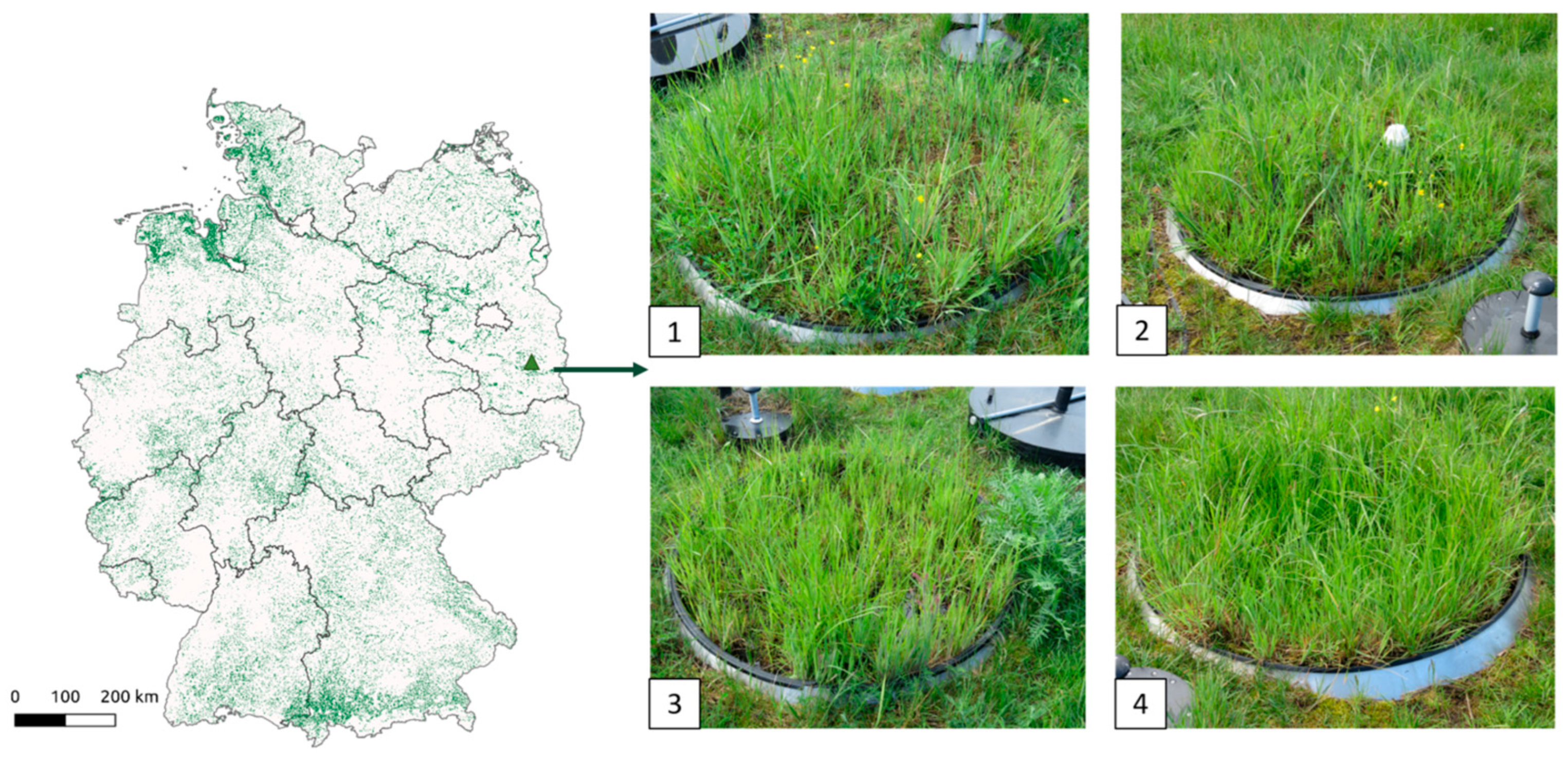
2.1. Study Area

The study area is an extensively agriculturally used wetland area in the Spreewald wet grassland, Germany (51°52′ N, 14°02′ E, and 50.5 m above sea level (Figure 1). The lysimeter station (container design) was installed in 2009 [35] and has been in operation since 2010; since then, the system has collected data, with the most recent available data coming from 2020. Since the recorded values for 2010 were only used for calibration purposes, the core data stemmed from spring 2011 to winter 2020 simultaneously from a weather station, a groundwater gauge, and a soil-hydrological measuring unit. The latter was equipped with tensiometers and frequency-domain reflectometry (FDR) probes to measure daily soil moisture at a depth of 30 cm.

2.2. Data

Four soil monoliths with a surface area of 1 m2 and 2 m depth were extracted directly from the site, and placed on a weighing system in four lysimeters (hereafter L1, L2, L3, and L4) [11,36]. We inserted the soil monoliths inside each lysimeter such that the soil profile remained undisturbed. Table 1 provides detailed information on the soil layer thickness and the soil properties at various soil layers of each lysimeter.
The water table depth (WTD) was measured on a daily basis in each lysimeter. Unlike conventional groundwater lysimeters that keep WTD at a constant value by controlling inflow and outflow [37,38], this station is equipped with an automatic control system for WTD. This facilitates the investigation of different WTD regimes that have a natural annual cycle and the effect the WTD regime has on water chemistry and vegetation. Overall, the WTD time series included 1.1% missing values, which we filled using polynomial interpolation [39]. The WTDs in the lysimeters ranged between 165 cm below the surface in L2 and 8.2 cm above the surface in L4 (Table 1). We regulated the WTD dynamics in the individual lysimeters differently. In L1, we regulated these dynamics according to the measured WTD in the surrounding area (Figure 2). In L2, we consistently maintained a lower WTD than in the other lysimeters. As a result, L2 was the driest lysimeter (Figure 2). From 2011 to 2015, L2 underwent a great deal of regulation, with long phases of constant WTD. Similar management was applied in L3 from 2015 to 2018 [40]. However, from 2018 on, the WTD in L3 was regulated to mimic more moist conditions, incorporating the days when the surface was flooded (positive WTD values in Figure 2). L4 was operated as the wettest lysimeter, with a higher WTD in spring than in other seasons. As shown in Figure 2c,d, L3 and L4 include positive WTDs (flooded conditions), with a maximum WTD of 4.7 cm above the surface for L3 and 8.2 cm above the surface for L4.
Mowing was performed twice per growing season (mid-June, beginning of September). Above-ground biomass (AGB) was measured twice per growing season, after each mowing event [11]. We measured the leaf area index (LAI) approximately every two weeks, using the S1 SunScan Canopy Analysis System [35]. In addition, once a year before the first cut, we conducted a vegetation composition assessment based on the Braun–Blanquet approach [41], which uses the “extended rating scale” (Erweiterte Boniturskala, [42]. This method quantifies the changes in vegetation based on the frequency of species and a variety of vegetation indicators [43]. These indicators show under which conditions certain plants establish themselves better than others, along with ecological gradients. We selected two indices that represent two important growth conditions: soil moisture and nutrient availability. The first indicator is the wetness index (mFZ; mittlere Feuchtezahl), which ranges between 1 and 9. An mFZ of 1 refers to plants that tolerate extremely dry soils, whereas an mFZ of 9 refers to plants that thrive on very wet soils [44]. The second indicator is the nutrient index (mNZ; mittlere Nährstoffzahl). An mNZ value of 1 is representative of species that grow in extremely infertile soils, while an mNZ of 9 represents species that dominate in extremely nutrient-rich soils [45]. In most cases, nutrient availability, and thus mNZ as a response indicator, is dominated by nitrogen.

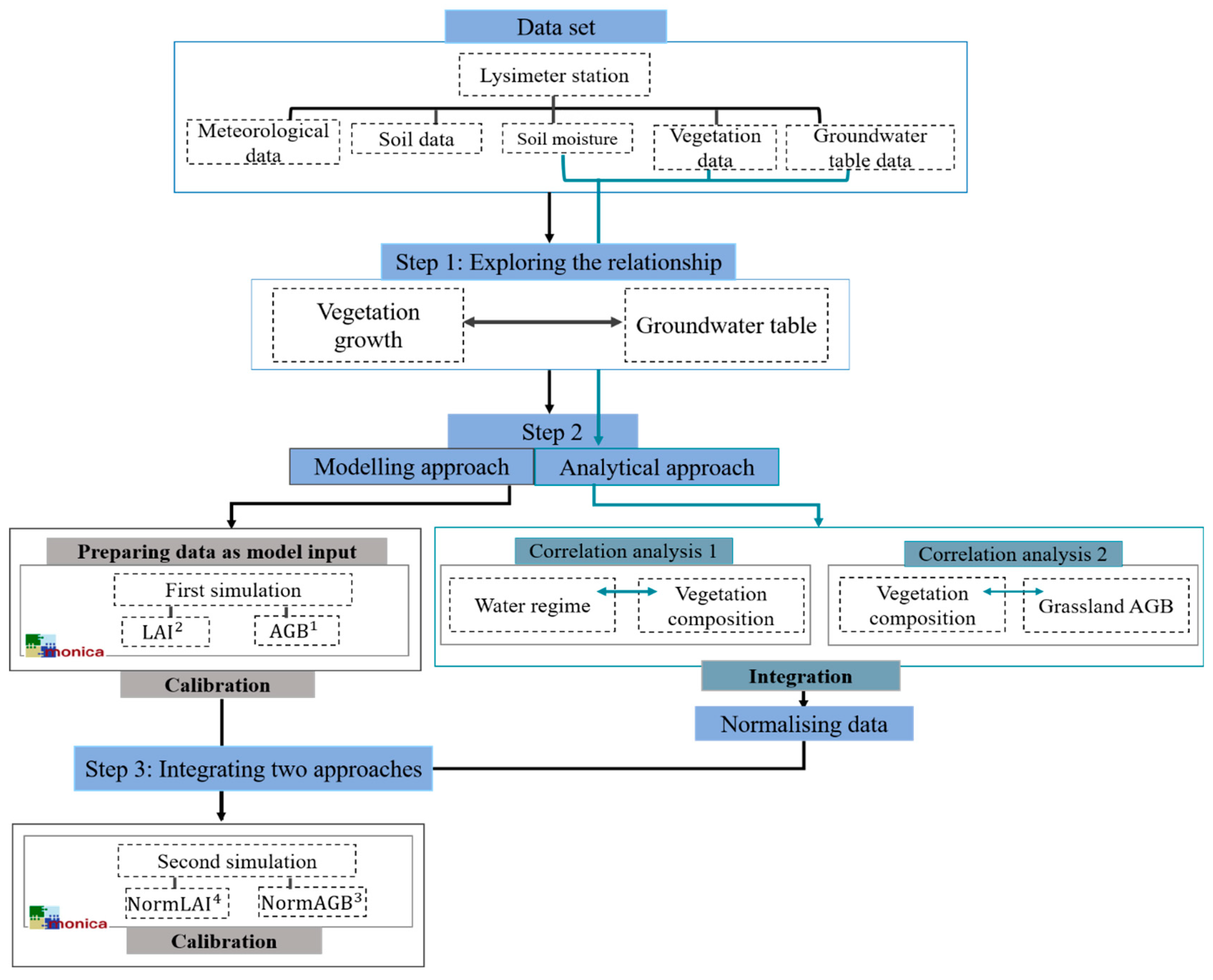
2.3. Exploring Relationships between WTD and Vegetation Growth

We explored how WTD dynamics affect vegetation growth using two parallel approaches (Figure 3): On the one hand, we used an AEM to simulate vegetation growth in response to changing WTDs (modelling approach); on the other hand, we used correlation analysis to investigate the relationship between vegetation growth and the water regime (analytical approach).

2.3.1. Modelling Approach

We used the MONICA model (MOdel for NItrogen and Carbon dynamics in Agroecosystems) to simulate the response of the grass vegetation’s growth to the soil moisture dynamics in the lysimeters. MONICA is an AEM that simulates the development and growth of a range of agricultural crops, including grassland, in conjunction with the water and nitrogen dynamics in the plant–soil–atmosphere continuum based on the underlying biophysical processes and in response to genotype, soil properties, weather, and agricultural management [46]. MONICA uses a capacity approach to simulate soil water dynamics based on [47]. This approach includes capacity parameters derived from the soil texture class [48]. Since the capacity approach only allows for downward water movements, we employed an empirical approach to investigate ascending water in the capillary fringe above the WTD, using daily rise rates from the German soil survey manual [48] as below.
h     j ( S )   θ i   +   1   =   θ i + C R R ( S ,   h )
h     j ( S )   θ i   +   1   =   θ i ,
where S is the soil texture, h is the distance between soil layer i and the top of the water table surface underground. CRR(S, h) denotes the capillary rise rate for soil type and distance from the top layer of the groundwater table; empirical values for these variables are taken from the German soil survey manual ([mm d−1] → [m3 m−3 d−1]; [48]). j(S) is the maximum distance between soil layer i and the top layer of the water table for which CRR exists [dm], and θ is the soil moisture [m3 m−3]. As a generic crop model, MONICA requires species-specific parameters to represent the growth and development of a specific plant. For multi-species grass vegetation, we calibrated parameters to observe growth patterns, as previously described by Kamali [49].
MONICA is in principle capable of simulating the vegetation growth response to water availability, with a positive response up to an optimum soil moisture content (around field capacity), and a negative response once soil moisture contents exceed this optimum towards full saturation, at which point the lack of oxygen in the rhizosphere impedes vegetation growth (Figure 4).
We calibrated MONICA using a calibration procedure based on the SUFI2 sequential uncertainty fitting algorithm [50,51]. In the SUFI2 algorithm, possible sources of uncertainty (parameters, conceptual model, input, etc.) are quantified by expressing a range between 2.5% and 97.5% uncertainty bounds (95% prediction uncertainty 95PPU; [51]). The 95PPU is obtained through Latin Hypercube sampling in the range of the parameter (a sample size of 500 for each lysimeter). The algorithm calculates the average of the objectives and considers them as single final values for optimisation. We used two indices to evaluate model performance [52]: the p-factor is the fraction of measured data (plus its error) bracketed by the 95PPU band and ranges between 0 and 1, where 1 signifies a perfect simulation in light of uncertainty [53]. The r-factor is the average width of the 95PPU band divided by the standard deviation of the measured variable; it is a measure of prediction uncertainty with 0 signifying the perfect simulation [53]. We also calculated the relative root-mean-square error (rRMSE) and the Willmott [54] index of agreement d as standardised measures of the degree of model prediction error. From the whole dataset, the data from 2014 to 2019 was selected as the calibration dataset. The parameters selected for model calibration were taken from Kamali [49].

2.3.2. The Analytical Approach

We took a two-step approach to investigate the relationship between the water regime and vegetation growth. First, we used a heat map graph to analyse the relationship between AGB and the two crucial components of the water regime: WTD and soil moisture (SM). To do so, the SM and WTD data, characterised by substantial damping and delay, was assessed by low-pass filtering of the time series (Equations (3) and (4); [55]). The objective was to understand how intensely the water regime influences vegetation growth in wet grassland with a shallow WTD. Since vegetation does not respond quickly to water regime components [56], we conducted another round of correlation analysis for AGB and the one-year time-lagged WTD and SM values.
x t i = k = n 2 + 1 n 2   e 2 i k n a ^ k ,
where
a ^ k = a k . a k n / 2 b .
and n is the number of data points x t i at dates   t i , the degree of low pass filtering a k is adjusted using coefficient b, (b = 0 means no filtering) for different frequencies k.
The second step was designed to investigate the effect of constantly changing vegetation composition (mFZ and mNZ) on AGB. Since mFZ and mNZ were only measured before the first cut, we investigated the relationship between the AGB measurements from the first cut and the two measurements of vegetation composition (mFZ and mNZ).

2.3.3. Integrating the Simulation and the Analysis

A mechanistic simulation model for plant growth processes such as MONICA should be able to simulate growth patterns in response to soil moisture dynamics, as demonstrated in Figure 4. However, this concept is founded on the assumption that the parameters describing species composition remain constant during the simulation. In our experiment, this was not the case, as the species composition in the grassland vegetation changed in response to medium-term water regime patterns. The lysimeter grassland vegetation constituted different species, each with a unique growth pattern and biomass performance (and thus the requirement for individual growth parameters in MONICA). As a consequence, the biomass-to-water regime response is blurred by the species-composition-to-water regime response signal. To enable MONICA to explain the biomass dynamics in response to soil moisture, both signals first need to be disaggregated.
To this end, we removed the species-composition-to-water regime response signal from the AGB and LAI time series to create a dataset that only included the biomass-to-water regime and the LAI-to-water regime response signal. The change in species composition was factored out by fitting a linear regression function to the AGB time series (Equation (5)) and to the LAI time series (Equation (6)). These normalised AGB and normalised LAI regressions are referred to as NormAGB and NormLAI, respectively.
N o r m A G B = A G B a + b × m F Z
N o r m L A I = L A I a + b × m F Z .
Since mFZ and mNZ were closely correlated, it was not necessary to remove the nutrient effect on species composition.

3. Results

3.1. The Response of Above-Ground Biomass to Groundwater Table Dynamics

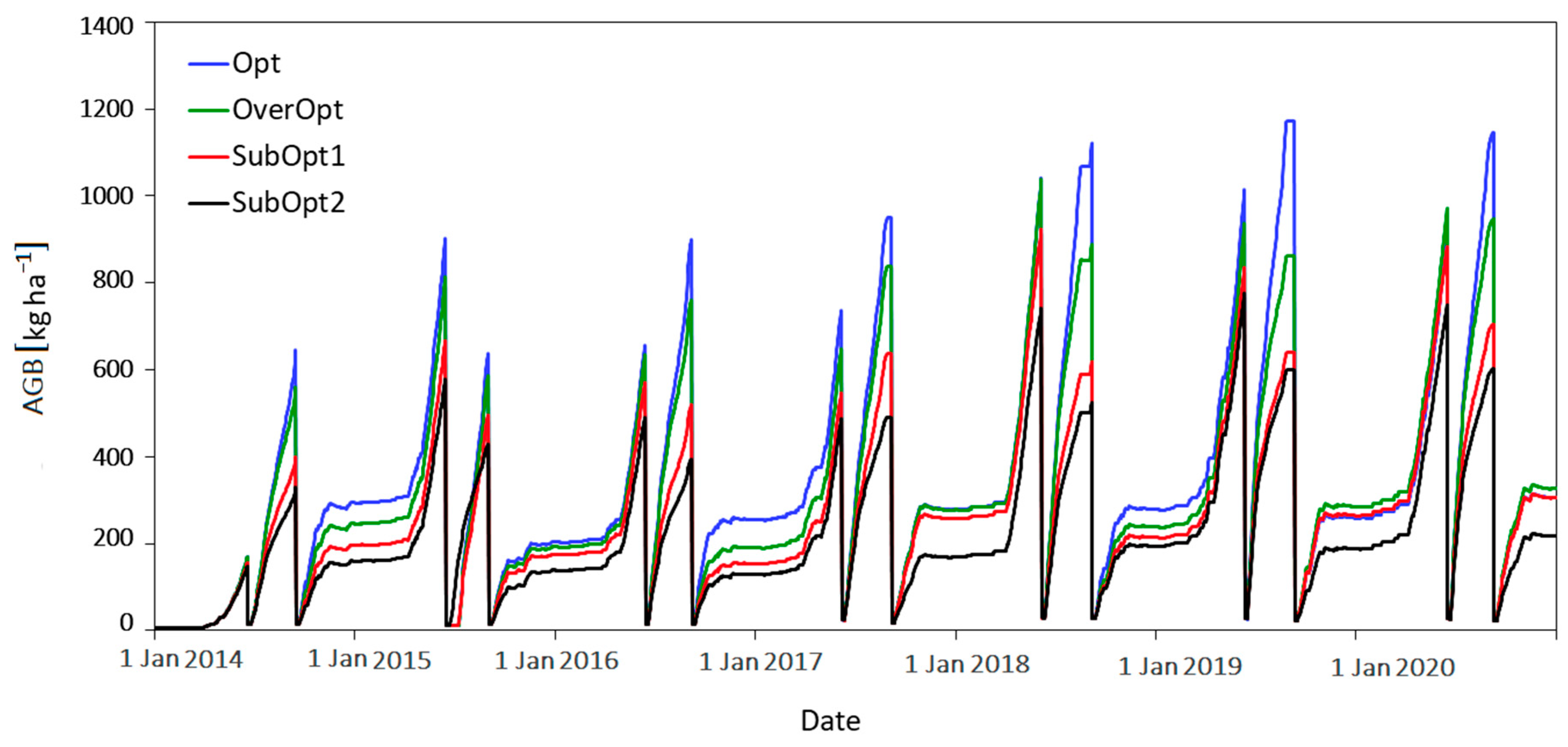
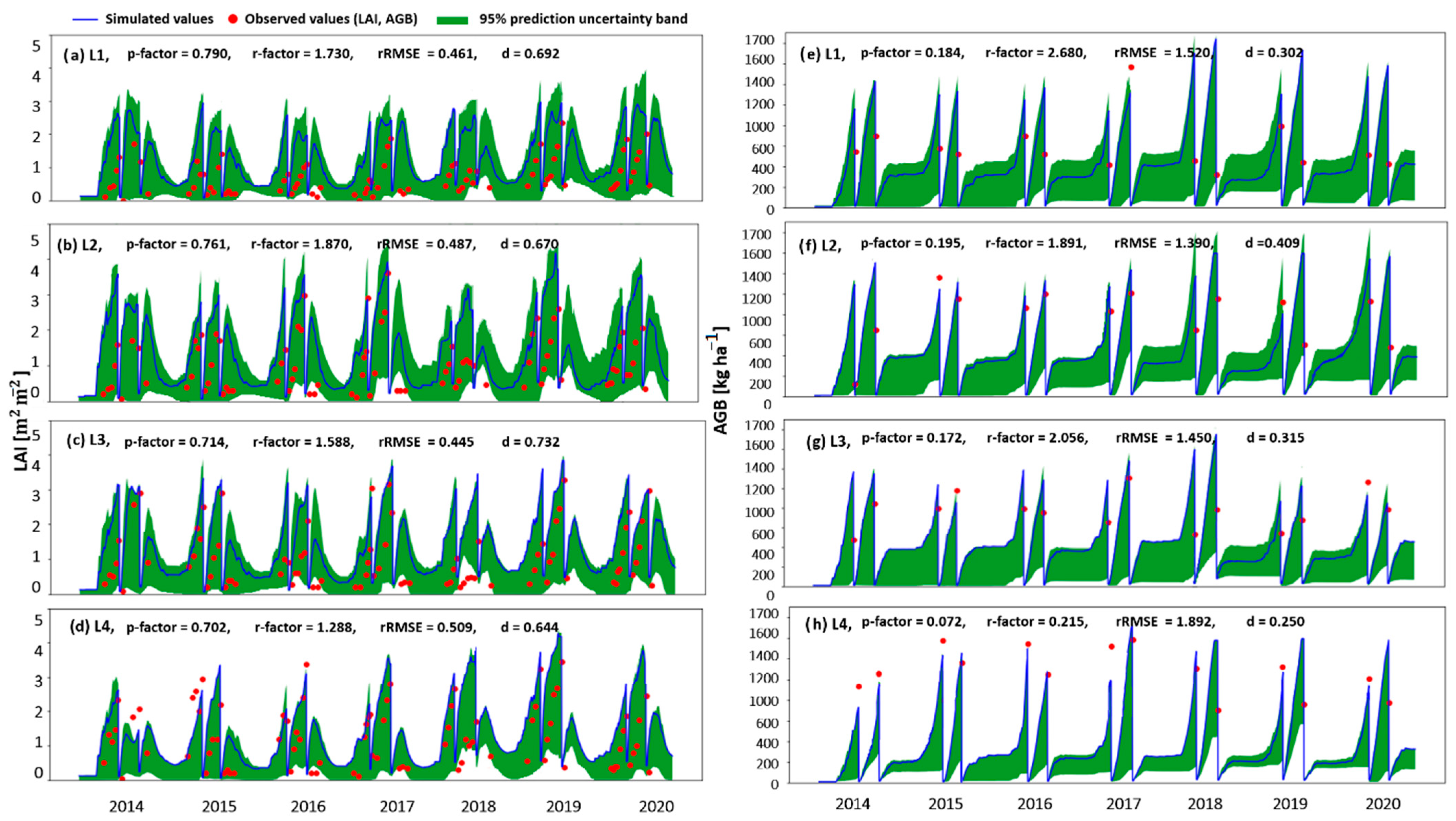
3.1.1. The Modelling Approach

First, we evaluated the performance of the MONICA model’s LAI and AGB simulations based on the original LAI and AGB time series. Our results showed significant variability in model performance across lysimeters, indicating different model performances for LAI and AGB (Figure 5). Specifically, for LAI, the results demonstrated an overestimation in all lysimeters during the year with the lowest precipitation (Table S1 in Supplementary Materials) and deepest WTD in 2018. Conversely, in the lysimeter with the wettest conditions (L4), LAI was underestimated in 2015 and 2016; similarly, in L3 during the wettest year (2017); Figure 5c. The best match of LAI was found in L3, with the lowest rRMSE of 0.445 and a p-factor of 0.714. The highest p-factor occurred in L1 (Figure 5a), which had the second-lowest rRMSE of 0.461. In L2 (Figure 5b), the MONICA model overestimated LAI in 2014, 2018, and 2020, while in 2016 and 2017, it was well-captured. However, during the second mowing period of 2014 and 2016, and the first mowing period of 2015, LAI was underestimated for L4 (Figure 5d), resulting in the highest rRMSE of 0.509, and the lowest p-factor of 0.702. Despite the variability in model performance across lysimeters, the simulated LAI values came close to the observed values (d = 0.69).
In contrast to LAI, the model’s performance in simulating AGB was unsatisfactory. The worst performance was seen in L4, where the model consistently underestimated AGB for almost all years and mowing events, with the highest rRMSE of 1.892. The simulation of AGB did not match the observed AGB well, as indicated by low p-factor values ranging from 0.072 in L4 (Figure 5h) to 0.195 in L2 (Figure 5f). The rRMSE results were also unacceptably high, ranging from 1.89 in L4 to 1.39 in L2. The AGB values in 2015 in L2 and L4 (Figure 5f,h) and in 2017 in L1 and L4 (Figure 5e,h) were underestimated. In 2018, AGB was overestimated in all lysimeters. An overall underestimation was observed in L4, except for 2015. In summary, the model slightly overestimated AGB under dry conditions and underestimated it during wet conditions (d = 0.30).

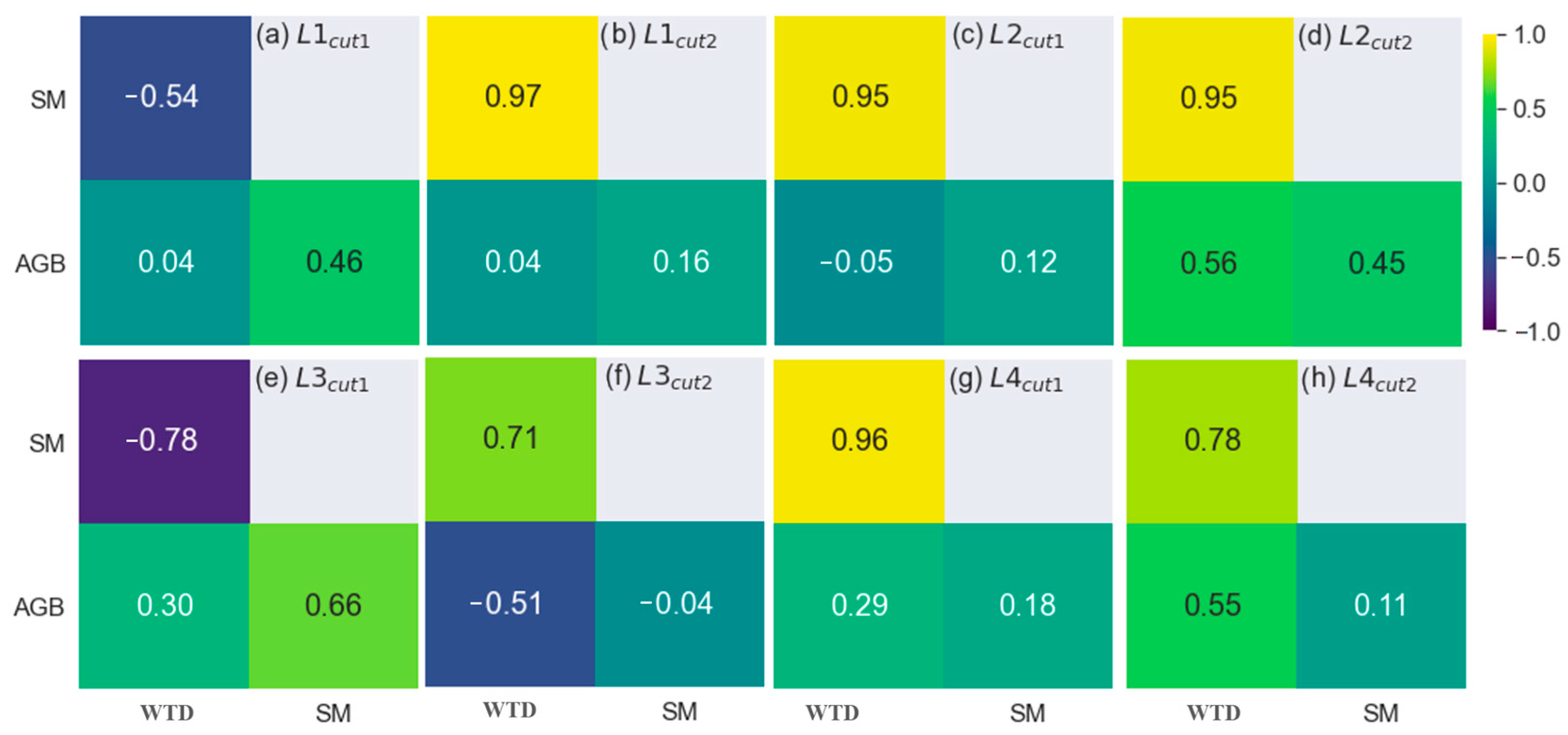
3.1.2. The Analytical Approach

With this unsatisfying result for AGB simulations, we were interested in learning more about the direct and indirect factors that influenced the growth dynamics of the grass vegetation in the lysimeters. For this purpose, we conducted a correlation analysis between the water regime (WTD and SM) and AGB (direct factor) (Figure 6). The initial results showed no strong correlation for any year (Figure 6). However, when taking a more detailed look, the response of AGB to WTD may vary from one mowing event to another. We therefore looked at correlations to the first cut (Cut1) and the second cut (Cut2) per season separately. Although correlation values were higher for the second mowing event, the relationship between WTD and AGB was fairly poor (Figure 6).
Inspired by the empirical observations from the lysimeters, we investigated the response of AGB to the water regime under consideration of a time lag by calculating the performance indices between AGB, WTD, and SM. There, ABG showed a considerably stronger correlation relationship with WTD and SM in both mowing periods (Figure 7). The highest correlation during the first cut was found in L3 and L4, with a coefficient of r = 0.97 between AGB and one-year lagged WTD (Figure 7c). We conclude at this stage that the vegetation’s AGB does not respond immediately to the change in the water regime, but requires more time to react, with visible effects appearing in the following season.

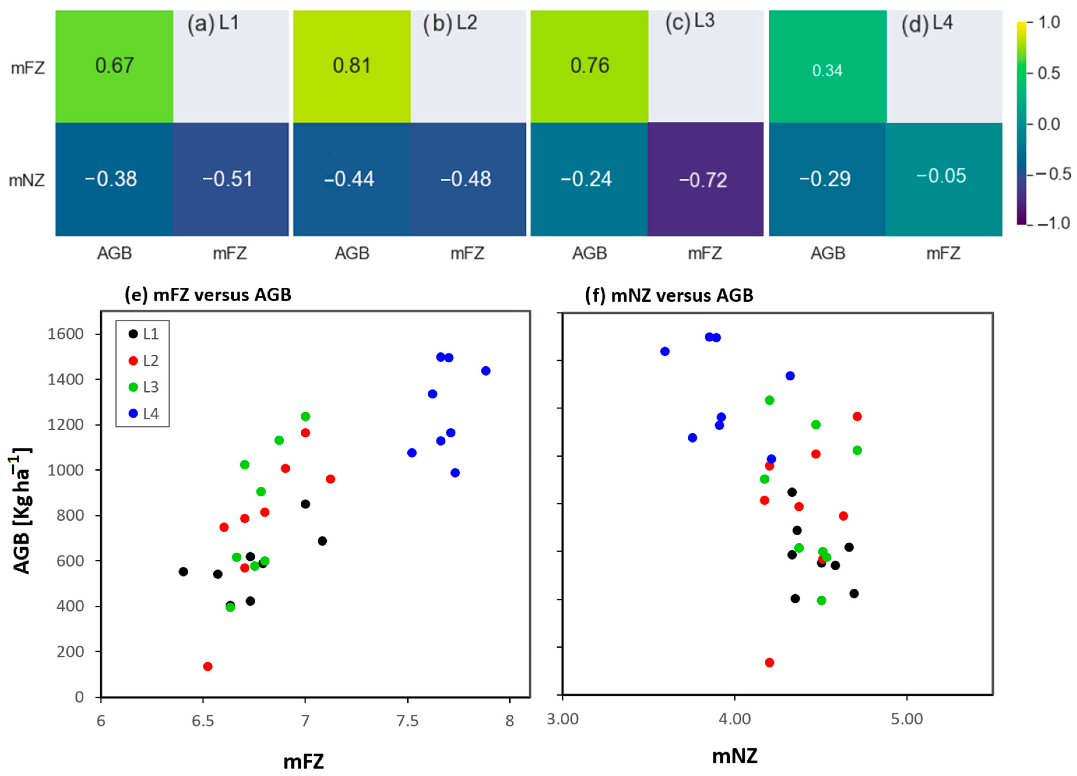
3.2. Response of Species Composition to Groundwater Table Dynamics

Species composition in the lysimeters significantly responded to changes in the water regime after a one-year time lag. We conducted a second series of correlation analyses using mFZ, mNZ, and AGB (as shown in Figure 8). The results revealed a significant positive relationship between mFZ and AGB in all lysimeters, with the highest Pearson correlation coefficient, r = 0.81 observed in L2 (Figure 8b) and the lowest correlation coefficient, r = 0.3 in L4 (Figure 8d). Conversely, AGB showed a negative correlation relationship with mNZ, with Pearson correlation coefficients ranging from −0.44 for L2 (Figure 8b) to −0.24 for L3 (Figure 8c).

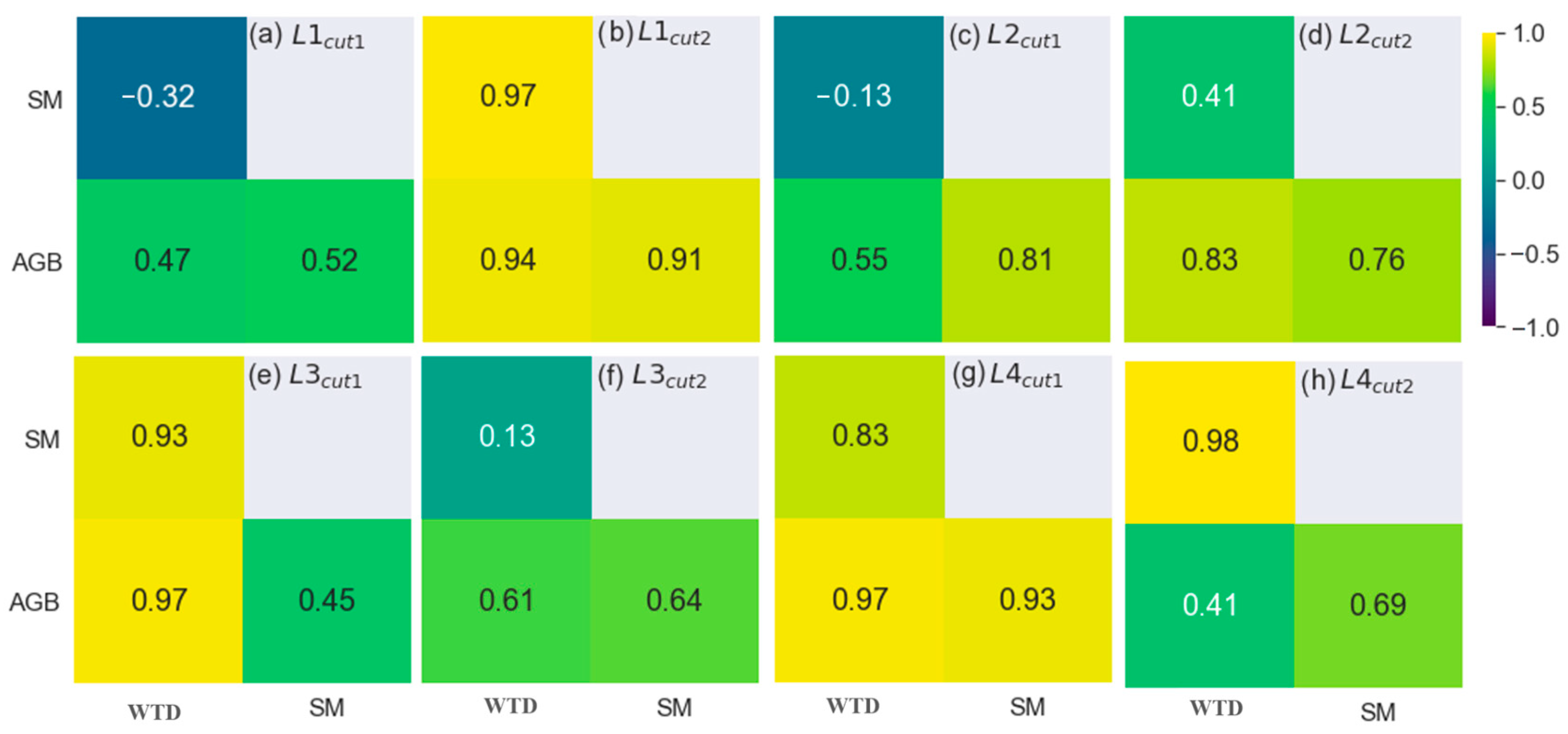
3.3. Integrating the Modelling Approach and the Correlation Analysis

The results of the analytical approach (Figure 6, Figure 7 and Figure 8) indicated a strong relationship between mFZ and AGB. Furthermore, the effect of the water regime on AGB values became apparent after one year, as the water regime positively influenced AGB through changes in species composition reflected by mFZ over the course of one year. Simultaneously, the results from the modelling approach showed that the model did not accurately reflect the annual variation in AGB. At this point, we hypothesise that the species composition change, exhibiting different biomass growth patterns, interferes with the direct relation between AGB and the water regime. To test this hypothesis, we conducted another MONICA simulation with an LAI and AGB dataset. We removed the WTD effect on species composition after fitting a linear regression derived from the linear relationship between mFZ and AGB (Figure 8). After factoring out the effect of mFZ from AGB and LAI, a modified (normalised) LAI and AGB dataset was available for the new series of simulations.
MONICA was calibrated against the normalised values for LAI and AGB (Figure 9a–d). The simulation results for LAI changed slightly from the previous simulation, but there was a negligible decline in rRMSE from 0.461 to 0.45 in L1, from 0.487 to 0.471 in L2, from 0.445 to 0.441 in L3, and from 0.509 to 0.507 in L4. In the second series of LAI simulations, the best match between simulations and normalised values was still in L3, which had the lowest rRMSE (0.441). The overall d for LAI in the second series of simulations was 0.71. The AGB simulations subsequently resulted in a closer match compared to the initial calibrated simulation. The best match was found at L2, with a p-factor of 0.412 and an rRMSE of 0.71 (Figure 9b). The model improved in capturing the lowest normalised AGB in 2014 in L2, which was previously overestimated in the initial simulation. The simulation for L3 resulted in a p-factor of 0.335 and an rRMSE of 0.79, making it the second-best match for normalised AGB after L2. L1 showed a significant improvement in its AGB simulation compared to the initial simulation, with a p-factor increase from 0.184 (Figure 5a) to 0.95 (Figure 9d). L4 also improved, but to a far lesser extent, with a p-factor increase from 0.071 (Figure 5d) to 0.142 (Figure 9d). The overall d of AGB simulation for all lysimeters throughout the calibration period increased to 0.45 (Table 2). In contrast, the improvement in the LAI measurement was negligible after removing the effect of water regime change on species composition.

4. Discussion

4.1. The Impact of Water Regime on Biomass Growth

The goal of this study was to test how well MONICA simulates biomass growth dynamics in wet grasslands that are strongly influenced by groundwater dynamics, including frequent flooding. We found that the simulation of ABG was initially poor, even though the relevant processes describing biomass response to water availability and soil moisture, including oxygen stress during flooded conditions, are featured in the model. Correspondingly, the correlation analysis revealed a poor correlation between AGB and the water regime dynamics, corroborating earlier studies [14,57,58]. In general, grassland species exhibit the ability to tolerate frequent mowing or grazing by resprouting soon after the disturbance [59]. Carbon allocation to the different plant organs during regrowth is highly influenced by soil water availability, leading to greater investment in roots and shoots during drought, and correspondingly less in leaves, for many grassland species [60]. This allocation pattern contributes to lower AGB development under dry conditions, while the general reduction in photosynthesis under limited water supply adds to the effect. Photosynthesis, however, regains its full rate as soon as the water supply returns to its optimum, while the carbon invested in roots and stems remains irreversible within a certain period. Even if the plant allocates assimilates from photosynthesis to leaves again after the water supply has returned to its optimal level, the biomass gap (difference from the potential biomass) cannot be compensated for until the next mowing event. A drought period followed by a period of ample water supply will therefore lead to lower AGB yields compared to the same period in reverse sequence. At the same time, high water supply levels towards the end of the season are more likely to leave soil moisture fully replenished over winter until spring, supplying the new season’s regrowth with water and supporting the microbial turnover process in soil, which eventually results in the availability of more nutrients. In contrast, the effects of a late-season drought may well reach into the next year’s growing season, with less water being available in the soil profile as well as fewer nutrients being released from soil organic matter due to suboptimal conditions for microbes. All these considerations may contribute to explaining why AGB yields correlate with the water supply condition of the previous year rather than the current one.

4.2. The Impact of Water Regime on Grassland Species Composition

Numerous studies have suggested that water table depth and soil moisture levels are the primary determinants of species composition in wet grasslands [61,62,63]. Plants develop different strategies to cope with stresses related to water. Hygrophyte species (e.g., Carex, Agrostis, Festuca) tolerate wet soils and frequent flooding, while mesophyte species (e.g., Poa, Lolium, Anthoxanthum) do not [64,65]. On sandy patches, longer drought may even lead to the establishment of more drought-tolerant species (e.g., Cichorium, Dactylis). Xu [14] showed that there is a positive significant correlation between species composition and soil moisture. This confirms the findings in our study, where the mFZ of the vegetation correlated positively with the water regime (groundwater table and soil moisture), albeit after a time lag of one year (see Section 4.1). Furthermore, our result confirms the suitability of the mFZ as an indicator for a wetness gradient in the species composition of wetlands.

4.3. The Indirect Relationship between Water Regime and Biomass Growth

It is well known that different grassland species differ with regard to annual biomass growth. However, how changes in species composition interact with the productivity of grassland is less documented because of the limited availability of data on species composition, as well as the incorporation of these data into biomass production models [66,67]. There are no mono-species permanent grassland, and the yield potential of grassland is often a matter of multifaceted interspecies feedback relationships, rather than the independent effects of individual constituents [68]. In our study, we document at least a correlation between the wetness index of species composition and AGB. The simultaneous correlation between the nutrient index of species composition and AGB is most likely explained by the increasing potential for denitrification at soil moisture levels above field capacity [69] and nitrogen losses into the atmosphere that are affected by this process. The decreasing availability of nitrogen is an additional cause that would influence species composition, as our data shows. However, this decrease in nitrogen is indirectly caused by the changes in soil moisture, rather than an independent process, which confirms the findings of the [32] study for upland grassland sites.

4.4. Simulating the Processes Leading to the Grassland Yield Pattern Observed

Grassland biomass responds to water availability, nitrogen availability, temperature, and radiation. These effects are nonlinear and interact in various ways. The resulting feedback control system is highly complex, and behaviour cannot be easily disaggregated. AEMs such as MONICA have nevertheless been designed to reproduce the behaviour of such systems. MONICA reproduces the yield-promoting effect of increasing soil moisture availability up to field capacity as well as the yield-degrading effect of soil moisture levels exceeding field capacity, which corresponds to the decrease in oxygen availability in soil. Furthermore, MONICA is also designed to reproduce soil organic matter turnover, nitrification, and denitrification in response to soil moisture levels, soil mineralogy, and temperature; this ensures that the indirect effect of soil moisture on plant growth (because of moisture’s relationship with nitrogen availability) is also reproduced. Finally, MONICA also simulates ascending soil moisture in the unsaturated fringe above WTD, the survival of grass stolons over winter to regrow in the following season, and the necrosis/senescence of root and leaf parts on a daily basis [49]. All in all, when we approached the task of simulating vegetation growth dynamics in response to changing groundwater levels, we did so under the assumption that MONICA would be fit for this purpose.
The first calibration of MONICA to the observed data using SUFI2 revealed relatively weak performances for AGB dynamics across all four lysimeters, with no clear tendency for over- or underestimation of the observed data. On the other hand, the LAI simulations already showed a fair performance (Figure 6). Any comparison between those two variables is, however, hampered by the fact that LAI was observed much more frequently than AGB. Visual inspection of the vegetation led to a new hypothesis; we introduced the non-permanence of vegetation composition as a factor that may have reduced MONICA’s accuracy, since an important precondition for the model’s application (constant vegetation properties) had obviously been violated. At that stage, it was not possible to introduce a new feature into MONICA that could simulate the change of the composition of a multispecies community over time. For that reason, we decided to modify the observation dataset instead and remove the effect of the changing species composition. Repeating the simulations for all four lysimeters against the modified (normalised) dataset revealed a better match between simulations and data for AGB in general (Table 2).

5. Conclusions

The AEM MONICA had significant difficulties in reproducing the original dataset that had been influenced by groundwater fluctuations, weather, and the subsequent changes in species composition. It performed much better in simulating AGB after the effect of species composition dynamics had been removed, which confirms the findings of earlier studies in upland grassland sites [33,70]. As hypothesised, the use of MONICA as a typical representative of AEMs to simulate the biomass production and related ecosystem services and disservices simultaneously across different grassland types, including wet grasslands with varying groundwater levels, is likely to produce fairly inaccurate results, while it works well as long as the species composition remains constant. As a consequence, the MONICA model needs to incorporate species composition dynamics for the simulation of wet grasslands, as previously suggested by Moulin [32] for their DynaGraM grassland model for upland grassland sites. Such competition models already exist and could be considered as complementary models that could be merged with MONICA in the future. One such example is the GRASSMIND model [71,72], which simulates plant growth and dynamics of species-rich grasslands, under consideration of the competition between individual plants for light, space, soil water, and nitrogen, different management regimes (e.g., mowing, irrigation, fertilisation) and varying weather conditions. Coupling GRASSMIND to a process-based soil model has already been attempted [73], but not yet in a full feedback loop to update plant growth characteristics. However, combining MONICA and GRASSMIND appears to be a realistic approach to better predictions of grassland yields in light of shallow groundwater dynamics.

Supplementary Materials

The following supporting information can be downloaded at: https://www.mdpi.com/article/10.3390/agriculture14050679/s1, This study contain a supplementary file that describes how wet or dry was each year in: Table S1: Mean annual air temperature, precipitation and FAO grassland reference evapotranspiration in the period from 2011 to 2020. Reference [74] is cited in the Supplementary Materials.

Author Contributions

V.K.: Conceptualization, Methodology, Writing—Original draft preparation. Visualisation, Investigation. B.K.: Software, Investigation, Writing—Reviewing and Editing, Model calibration. G.L.: Data analysis, Visualization, Investigation, Writing—Reviewing and Editing, Supervision. O.D.: Data curation, Writing—Reviewing and Editing. M.F.D.: Data curation. C.N.: Motivation, Supervision, Software, Writing—Reviewing and Editing, Conceptualisation, Investigation, Software. All authors have read and agreed to the published version of the manuscript.

Funding

Funding for this research was provided by the Leibniz Centre for Agricultural Landscape Research through its Integrated Priority Project entitled “Water and carbon dynamics in agriculturally used wetlands” (ID 2196).

Institutional Review Board Statement

Not applicable.

Data Availability Statement

Data available in a publicly accessible repository. The data presented in this study are openly available in [BONARES] at [https://doi.org/10.4228/zalf-vevz-ys85], accessed on 22 April 2024, reference number [WGS84].

Conflicts of Interest

We declare that there are no conflicts of interest related to the submitted manuscript [“Challenges of including wet grasslands with variable ground-water tables in large-area crop production simulations”].

References

  1. White, R.P.; Murray, S.; Rohweder, M.; Prince, S.D.; Thompson, K.M. Grassland Ecosystems 2000; World Resources Institute: Washington, DC, USA, 2000; p. 81. [Google Scholar]
  2. Zhu, H.; Fu, B.; Wang, S.; Zhu, L.; Zhang, L.; Jiao, L.; Wang, C. Reducing soil erosion by improving community functional diversity in semi-arid grasslands. J. Appl. Ecol. 2015, 52, 1063–1072. [Google Scholar] [CrossRef]
  3. Myers, N.; Mittermeier, R.A.; Mittermeier, C.G.; Da Fonseca, G.A.; Kent, J. Biodiversity hotspots for conservation priorities. Nature 2000, 403, 853–858. [Google Scholar] [CrossRef]
  4. Wu, J. Landscape sustainability science: Ecosystem services and human well-being in changing landscapes. Landsc. Ecol. 2013, 28, 999–1023. [Google Scholar] [CrossRef]
  5. Joyce, C.B.; Wade, P.M. European Wet Grasslands: Biodiversity, Management and Restoration; John Wiley and Sons Ltd.: Chichester, UK, 1998. [Google Scholar]
  6. Cebrián-Piqueras, M.Á. Trade-Offs and Synergies between Forage Production, Species Conservation and Carbon Stocks in Temperate Coastal Wet Grasslands. An Ecosystem Services and Process-Based Approach. Ph.D. Dissertation, University of Oldenburg, Oldenburg, Germany, 2017. [Google Scholar]
  7. Hooper, D.U.; Chapin, F.S., III; Ewel, J.J.; Hector, A.; Inchausti, P.; Lavorel, S.; Lawton, J.H.; Lodge, D.M.; Loreau, M.; Naeem, S.; et al. Effects of biodiversity on ecosystem functioning: A consensus of current knowledge. Ecol. Monogr. 2005, 75, 3–35. [Google Scholar] [CrossRef]
  8. Cardinale, B.J.; Gross, K.; Fritschie, K.; Flombaum, P.; Fox, J.W.; Rixen, C.; Van Ruijven, J.; Reich, P.B.; Scherer-Lorenzen, M.; Wilsey, B.J. Biodiversity simultaneously enhances the production and stability of community biomass, but the effects are independent. J. Ecol. 2013, 94, 1697–1707. [Google Scholar] [CrossRef]
  9. Kennedy, M.P.; Milne, J.M.; Murphy, K.J. Experimental growth responses to groundwater level variation and competition in five British wetland plant species. Wetl. Ecol. Manag. 2003, 11, 383–396. [Google Scholar] [CrossRef]
  10. Reyer, C.P.; Leuzinger, S.; Rammig, A.; Wolf, A.; Bartholomeus, R.P.; Bonfante, A.; De Lorenzi, F.; Dury, M.; Gloning, P.; Abou Jaoudé, R.; et al. A plant’s perspective of extremes: Terrestrial plant responses to changing climatic variability. Glob. Chang. Biol. 2013, 19, 75–89. [Google Scholar] [CrossRef]
  11. Dietrich, O.; Behrendt, A.; Wegehenkel, M. The water balance of wet grassland sites with shallow water table conditions in the north-eastern German lowlands in extreme dry and wet years. Water 2021, 13, 2259. [Google Scholar] [CrossRef]
  12. Dwire, K.A.; Kauffman, J.B.; Baham, J.E. Plant species distribution in relation to water-table depth and soil redox potential in montane riparian meadows. Wetlands 2006, 26, 131–146. [Google Scholar] [CrossRef]
  13. Toogood, S.E.; Joyce, C.B. Effects of raised water levels on wet grassland plant communities. Appl. Veg. Sci. 2009, 12, 283–294. [Google Scholar] [CrossRef]
  14. Xu, X.; Zhang, Q.; Tan, Z.; Li, Y.; Wang, X. Effects of water-table depth and soil moisture on plant biomass, diversity, and distribution at a seasonally flooded wetland of Poyang Lake, China. Chin. Geogr. Sci. 2015, 25, 739–756. [Google Scholar] [CrossRef]
  15. Destatis, Statistisches Bundesamt. Land- und Forstwirtschaft, Fischerei. Bodenfläche nach Art der Tatsächlichen Nutzung; Fachserie 3 Reihe 5.1; Destatis, Statistisches Bundesamt: Wiesbaden, Germany, 2019. [Google Scholar]
  16. Roßkopf, N.; Fell, H.; Zeitz, J. Organic soils in Germany, their distribution and carbon stocks. Catena 2015, 133, 157–170. [Google Scholar] [CrossRef]
  17. Söder, M.; Berg-Mohnicke, M.; Bittner, M.; Ernst, S.; Feike, T.; Frühauf, C.; Golla, B.; Jänicke, C.; Jorzig, C.; Leppelt, T.; et al. Klimawandelbedingte Ertragsveränderungen und Flächennutzung (KlimErtrag); Johann Heinrich von Thünen-Institut: Braunschweig, Germany, 2022. [Google Scholar]
  18. Hetzer, J.; Huth, A.; Taubert, F. The importance of plant trait variability in grasslands: A modelling study. Ecol. Model. 2021, 453, 109606. [Google Scholar] [CrossRef]
  19. Robertson, A.D.; Paustian, K.; Ogle, S.; Wallenstein, M.D.; Lugato, E.; Cotrufo, M.F. Unifying soil organic matter formation and persistence frameworks: The MEMS model. Biogeosciences 2019, 16, 1225–1248. [Google Scholar] [CrossRef]
  20. Sándor, R.; Barcza, Z.; Hidy, D.; Lellei-Kovács, E.; Ma, S.; Bellocchi, G. Modelling of grassland fluxes in Europe: Evaluation of two biogeochemical models. Agric. Ecosyst. Environ. 2016, 215, 1–19. [Google Scholar] [CrossRef]
  21. Rahimi, J.; Haas, E.; Scheer, C.; Grados, D.; Abalos, D.; Aderele, M.O.; Mathiesen, G.; Butterbach-Bahl, K. Aggregation of activity data on crop management can induce large uncertainties in estimates of regional nitrogen budgets. Sustain. Agric. 2024, in press.
  22. Arango, M.A.; Anandhi, A.; Rice, C.W. Conceptual framework addressing timescale mismatch uncertainty: Nitrous-oxide (N2O) modeled and measured, Kansas, USA. Ecol. Model. 2023, 486, 110536. [Google Scholar] [CrossRef]
  23. Zhang, Y.; Lavallee, J.M.; Robertson, A.D.; Even, R.; Ogle, S.M.; Paustian, K.; Cotrufo, M.F. Simulating measurable ecosystem carbon and nitrogen dynamics with the mechanistically defined MEMS 2.0 model. Biogeosciences 2021, 18, 3147–3171. [Google Scholar] [CrossRef]
  24. Coffin, D.P.; Lauenroth, W.K. A gap dynamics simulation model of succession in a semiarid grassland. Ecol. Model. 1990, 49, 229–266. [Google Scholar] [CrossRef]
  25. Gillet, F. Modelling vegetation dynamics in heterogeneous pasture-woodland landscapes. Ecol. Model. 2008, 217, 1–18. [Google Scholar] [CrossRef]
  26. Siehoff, S.; Lennartz, G.; Heilburg, I.C.; Roß-Nickoll, M.; Ratte, H.T.; Preuss, T.G. Process-based modeling of grassland dynamics built on ecological indicator values for land use. Ecol. Model. 2011, 222, 3854–3868. [Google Scholar] [CrossRef]
  27. Thornley, J.H.M.; Verberne, E.L.J. A model of nitrogen flows in grassland. Plant Cell Environ. 1989, 12, 863–886. [Google Scholar] [CrossRef]
  28. Van Oijen, M.; Barcza, Z.; Confalonieri, R.; Korhonen, P.; Kröel-Dulay, G.; Lellei-Kovács, E.; Louarn, G.; Louault, F.; Martin, R.; Moulin, T.; et al. Incorporating biodiversity into biogeochemistry models to improve prediction of ecosystem services in temperate grasslands: Review and roadmap. Agronomy 2020, 10, 259. [Google Scholar] [CrossRef]
  29. Daleo, P.; Alberti, J.; Chaneton, E.J.; Iribarne, O.; Tognetti, P.M.; Bakker, J.D.; Borer, E.T.; Bruschetti, M.; MacDougall, A.S.; Pascual, J.; et al. Environmental heterogeneity modulates the effect of plant diversity on the spatial variability of grassland biomass. Nat. Commun. 2023, 14, 1809. [Google Scholar] [CrossRef]
  30. Jouven, M.; Carrère, P.; Baumont, R. Model predicting dynamics of biomass, structure and digestibility of herbage in managed permanent pastures. 1. Model description. Grass Forage Sci. 2006, 61, 112–124. [Google Scholar] [CrossRef]
  31. Clark, A.T.; Ann Turnbull, L.; Tredennick, A.; Allan, E.; Harpole, W.S.; Mayfield, M.M.; Soliveres, S.; Barry, K.; Eisenhauer, N.; de Kroon, H.; et al. Predicting species abundances in a grassland biodiversity experiment: Trade-offs between model complexity and generality. J. Ecol. 2020, 108, 774–787. [Google Scholar] [CrossRef]
  32. Moulin, T. Perasso, Antoine., Gillet, François., Modelling vegetation dynamics in managed grasslands: Responses to drivers depend on species richness. Ecol. Model. 2018, 374, 22–36. [Google Scholar] [CrossRef]
  33. Movedi, E.; Bellocchi, G.; Argenti, G.; Paleari, L.; Vesely, F.; Staglianò, N.; Dibari, C.; Confalonieri, R. Development of generic crop models for simulation of multi-species plant communities in mown grasslands. Ecol. Model. 2019, 401, 111–128. [Google Scholar] [CrossRef]
  34. Haas, E.; Klatt, S.; Fröhlich, A.; Kraft, P.; Werner, C.; Kiese, R.; Grote, R.; Breuer, L.; Butterbach-Bahl, K. LandscapeDNDC: A process model for simulation of biosphere–atmosphere–hydrosphere exchange processes at site and regional scale. Landsc. Ecol. 2013, 28, 615–636. [Google Scholar] [CrossRef]
  35. Dietrich, O.; Fahle, M.; Seyfarth, M. Behavior of water balance components at sites with shallow groundwater tables: Possibilities and limitations of their simulation using different ways to control weighable groundwater lysimeters. Agric. Water Manag. 2016, 163, 75–89. [Google Scholar] [CrossRef]
  36. Dietrich, O. Effects of Groundwater Levels and Soil Moisture on the Development of Leaf Area Index and Biomass Yield of Wet Grasslands (Lysimeter Data) [Data Set]; Leibniz Centre for Agricultural Landscape Research (ZALF): Müncheberg, Germany, 2023. [Google Scholar]
  37. Bethune, M.; Wang, Q.J.A. A lysimeter study of the water balance of border-check irrigated perennial pasture. Anim. Prod. Sci. 2004, 44, 151–162. [Google Scholar] [CrossRef]
  38. Noory, H.; Liaghat, A.M.; Chaichi, M.R.; Parsinejad, M. Effects of water table management on soil salinity and alfalfa yield in a semi-arid climate. Irrig. Sci. 2009, 27, 401–407. [Google Scholar] [CrossRef]
  39. Bos, L.; Caliari, M.; De Marchi, S.; Vianello, M. A numerical study of the Xu polynomial interpolation formula in two variables. Computing 2006, 76, 311–324. [Google Scholar] [CrossRef]
  40. Dietrich, O. Untersuchungen zum Wasserhaushalt Grundwassernaher Standorte Ergebnisse der Lysimeteranlage Spreewald; Programmbereich 2 “Landnutzung und Governance”, Arbeitsgruppe” Tieflandhydrologie und Wassermanagement; Leibniz-Zentrum für Agrarlandschaftsforschung (ZALF) e.V.: Müncheberg, Germany, 2021. [Google Scholar]
  41. Van der Maarel, E. The Braun-Blanquet approach in perspective. Vegetation 1975, 30, 213–219. [Google Scholar] [CrossRef]
  42. Mühlenberg, M.L. Freilandökologie, 2nd ed.; Quelle & Meyer: Heidelberg, Germany, 1989; p. 512. [Google Scholar]
  43. Ellenberg, H.; Leuschner, C. Vegetation Mitteleuropas mit den Alpen. In Öklogischer, Dynamischer und Historischer, 6th ed.; Ulmer UTB: Stuttgart, Germany, 2010. [Google Scholar]
  44. Barthelheimer, M.; Poschlod, P. Functional characterizations of E llenberg indicator values–a review on ecophysiological determinants. Funct. Ecol. 2016, 30, 506–516. [Google Scholar] [CrossRef]
  45. Berg, C.; Welk, E.; Jäger, E.J. Revising Ellenberg’s indicator values for continentality based on global vascular plant species distribution. Appl. Veg. Sci. 2017, 20, 482–493. [Google Scholar] [CrossRef]
  46. Nendel, C.; Berg, M.; Kersebaum, K.C.; Mirschel, W.; Specka, X.; Wegehenkel, M.; Wenkel, K.O.; Wieland, R. The MONICA model: Testing predictability for crop growth, soil moisture and nitrogen dynamics. Ecol. Model. 2011, 222, 1614–1625. [Google Scholar] [CrossRef]
  47. Wegehenkel, M. Test of a modelling system for simulating water balances and plant growth using various different complex approaches. Ecol. Model. 2000, 129, 39–64. [Google Scholar] [CrossRef]
  48. Eckelmann, W.; Sponagel, H.; Grottenthaler, W.; Hartmann, K.; Hartwich, R.; Janetzko, P.; Joisten, H.; Kühn, D.; Sabel, K.; Traidl, R. Manual of Soil Mapping (KA5), 5th ed.; Federal Institute for Geosciences and Natural Resources in cooperation with the State Geological Services: Berlin, Germany, 2005. [Google Scholar]
  49. Kamali, B.; Stella, T.; Berg-Mohnicke, M.; Pickert, J.; Groh, J.; Nendel, C. Improving the simulation of permanent grasslands across Germany by using multi-objective uncertainty-based calibration of plant-water dynamics. Eur. J. Agron. 2022, 134, 126464. [Google Scholar] [CrossRef]
  50. Abbaspour, K.; Rouholahnejad, E.; Vaghefi, S.; Srinivasan, R.; Yang, H.; Kløve, B. A continental-scale hydrology and water quality model for Europe: Calibration and uncertainty of a high-resolution large-scale SWAT model. J. Hydrol. 2015, 524, 733–752. [Google Scholar] [CrossRef]
  51. Abbaspour, K.C. SWAT-CUP: SWAT Calibration and Uncertainty Programs—A User Manual; Eawag: Dübendorf, Switzerland, 2015. [Google Scholar]
  52. Abbaspour, K.C.; CJohnson, A.; Van Genuchten, M.T. Estimating uncertain flow and transport parameters using a sequential uncertainty fitting procedure. Vadose Zone J. 2004, 3, 1340–1352. [Google Scholar] [CrossRef]
  53. Kamali, B.; Abbaspour, K.C.; Lehmann, A.; Wehrli, B.; Yang, H. Uncertainty-based auto-calibration for crop yield–the EPIC+ procedure for a case study in Sub-Saharan Africa. European J. Agron. 2018, 93, 57–72. [Google Scholar] [CrossRef]
  54. Willmott, C.J. On the validation of models. Phys. Geogr. 1981, 2, 184–194. [Google Scholar] [CrossRef]
  55. Lischeid, G.; Dannowski, R.; Kaiser, K.; Nützmann, G.; Steidl, J.; Stüve, P. Inconsistent hydrological trends do not necessarily imply spatially heterogeneous drivers. J. Hydrol. 2021, 596, 126096. [Google Scholar] [CrossRef]
  56. Liu, Y.; Yang, X.; Tian, D.; Cong, R.; Zhang, X.; Pan, Q.; Shi, Z. Resource reallocation of two grass species during regrowth after defoliation. Front. Plant Sci. 2018, 9, 1767. [Google Scholar] [CrossRef] [PubMed]
  57. Casanova, M.T.; Brock, M.A. How do depth, duration and frequency of flooding influence the establishment of wetland plant communities? Plant Ecol. 2000, 147, 237–250. [Google Scholar] [CrossRef]
  58. Zhang, J.T. Quantitative Ecology, 2nd ed.; Science Press: Beijing, China, 2011; Volume 77, pp. 82–92. [Google Scholar]
  59. Gibson, D.J. Grasses and Grassland Ecology; Oxford University Press: Oxford, UK, 2009. [Google Scholar]
  60. Hartmann, H.; Bahn, M.; Carbone, M.; Richardson, A.D. Plant carbon allocation in a changing world–challenges and progress: Introduction to a Virtual Issue on carbon allocation. New Phytol. 2020, 227, 981–988. [Google Scholar] [CrossRef] [PubMed]
  61. Baattrup-Pedersen, A.; JENSEN, K.M.; Thodsen, H.; Andersen, H.E.; Andersen, P.M.; Larsen, S.E.; Riis, T.; Andersen, D.K.; Audet, J.; Kronvang, B. Effects of stream flooding on the distribution and diversity of groundwater-dependent vegetation in riparian areas. Freshw. Biol. 2013, 58, 817–827. [Google Scholar] [CrossRef]
  62. Henszey, R.J.; Pfeiffer, K.; Keough, J.R. Linking surface-and ground-water levels to riparian grassland species along the Platte River in Central Nebraska, USA. Wetlands 2004, 24, 665–687. [Google Scholar] [CrossRef]
  63. Leyer, I. Predicting plant species’ responses to river regulation: The role of water level fluctuations. J. Appl. Ecol. 2005, 42, 239–250. [Google Scholar] [CrossRef]
  64. Brilli, F.; Hörtnagl, L.; Hammerle, A.; Haslwanter, A.; Hansel, A.; Loreto, F.; Wohlfahrt, G. Leaf and ecosystem response to soil water availability in mountain grasslands. Agric. For. Meteorol. 2011, 151, 1731–1740. [Google Scholar] [CrossRef] [PubMed]
  65. Symstad, A.J.; Wienk, C.L.; Thorstenson, A.D. Precision, repeatability, and efficiency of two canopy-cover estimate methods in northern Great Plains vegetation. Rangel. Ecol. Manag. 2008, 61, 419–429. [Google Scholar] [CrossRef]
  66. Krueger, E.; Ochsner, T.E.; Levi, M.R.; Basara, J.B.; Snitker, G.J.; Wyatt, B.M. Grassland productivity estimates informed by soil moisture measurements: Statistical and mechanistic approaches. Agronomy 2021, 113, 3498–3517. [Google Scholar] [CrossRef]
  67. Ortiz-Bobea, A.; Wang, H.; Carrillo, C.M.; Ault, T.R. Unpacking the climatic drivers of US agricultural yields. Environ. Res. Lett. 2019, 14, 064003. [Google Scholar] [CrossRef]
  68. Haughey, E.; Suter, M.; Hofer, D.; Hoekstra, N.J.; McElwain, J.C.; Lüscher, A.; Finn, J.A. Higher species richness enhances yield stability in intensively managed grasslands with experimental disturbance. Sci. Rep. 2018, 8, 15047. [Google Scholar] [CrossRef]
  69. Skiba, U. Denitrification. In Encyclopedia of Ecology; Jørgensen, S.E., Fath, B.D., Eds.; Elsevier: Oxford, UK; Academic Press: Oxford, UK, 2008; p. 866. [Google Scholar]
  70. Sándor, R.; Picon-Cochard, C.; Martin, R.; Louault, F.; Klumpp, K.; Borras, D.; Bellocchi, G. Plant acclimation to temperature: Developments in the pasture simulation model. Field Crop. Res. 2018, 222, 238–255. [Google Scholar] [CrossRef]
  71. Taubert, F.; Frank, K.; Huth, A. A review of grassland models in the biofuel context. Ecol. Model. 2012, 245, 84–93. [Google Scholar] [CrossRef]
  72. Taubert, F.; Hetzer, J.; Schmid, J.S.; Huth, A. The role of species traits for grassland productivity. Ecosphere 2020, 11, e03205. [Google Scholar] [CrossRef]
  73. Taubert, F. Modelling and Analysing the Structure and Dynamics of Species-Rich Grasslands and Forests; Helmholtz Centre for Environmental Research-UFZ, Department of Ecological: Leipzig, Germany, 2014. [Google Scholar]
  74. Allen, R.G.; Pereira, L.S.; Raes, D.; Smith, M. Crop Evapotranspiration: Guidelines for Computing Crop Water Requirements; Food and Agriculture Organization of the United Nations: Rome, Italy, 1998. [Google Scholar]
Figure 1. Location of the lysimeter station in the Spreewald wet grassland in Germany (left) and the vegetation coverage of the four lysimeters L1, L2, L3, and L4 (right, photos taken on 7 May 2019).
Agriculture 14 00679 g001
Figure 2. Daily fluctuation of water table depth from spring 2011 to 2020 in the lysimeters (L1 to L4: ad). The dashed line represents the soil surface.
Agriculture 14 00679 g002
Figure 3. Schematic flowchart of the steps for capturing wet grassland vegetation growth under a changing water table in three steps. 1 AGB (above-ground biomass); 2 LAI (leaf area index); 3 NormAGB (normalised above-ground biomass); 4 NormLAI (normalised leaf area index). The water regime includes soil moisture and water table data.
Agriculture 14 00679 g003
Figure 4. An artificial set-up illustrating different AGB simulations using MONICA with fixed groundwater tables at four different depths: (i) optimum groundwater distance for vegetation growth at 30 cm below the surface as obtained from a sensitivity analysis (Opt); (ii) above-optimum groundwater distance with a groundwater table at surface level (OverOpt); (iii) suboptimal groundwater distance with a groundwater table at 60 cm (SubOpt1); and (iv) 90 cm (SubOpt2) below surface. Weather data are taken from the weather station inside the lysimeter station for the period from 2014 to 2020.
Agriculture 14 00679 g004
Figure 5. MONICA simulation of LAI (ad), and simulated AGB (eh); dynamics versus observed LAI and AGB dynamics based on the data from the calibration period 2014–2020, in lysimeters L1–L4. Dots mark the observed values, the blue line the simulated values and the green area denotes the uncertainty band.
Agriculture 14 00679 g005
Figure 6. Pearson correlation analysis results between AGB, WTD, and soil moisture at 30 cm below-ground (SM) values for the first cut in the four lysimeters L1cut1–L4cut1 (a,c,e,g) and for the second cut L1cut2–L4cut2 (b,d,f,h).
Agriculture 14 00679 g006
Figure 7. Pearson correlation analysis results between AGB and the one-year time-lag WTD and soil moisture at 30 cm below-ground (SM) values for the first cut in four lysimeters L1cut1–L4cut1 (a,c,e,g) and for the second cut L1cut2–L4cut2 (b,d,f,h).
Agriculture 14 00679 g007
Figure 8. Relationships between AGB of the first cut, the mFZ and the mNZ were assessed separately using Pearson correlation coefficient in the four lysimeters (ad) and visualised for all lysimeters (e,f).
Agriculture 14 00679 g008
Figure 9. MONICA simulated LAI (ad), and AGB dynamics (eh); versus normalised observation for the period 2014–2020, in lysimeters L1–L4. Normalised values represent AGB and LAI data modified by removing the effect of the species composition. Dots mark the observed values, the blue line the simulated values and the green area denotes the uncertainty band.
Agriculture 14 00679 g009
Table 1. Soil properties and water table range in the lysimeters.
LysimeterSoil Layers (cm)Soil TypeWater Table Depth (WTD) (Shallowest to Deepest Values) (cm)
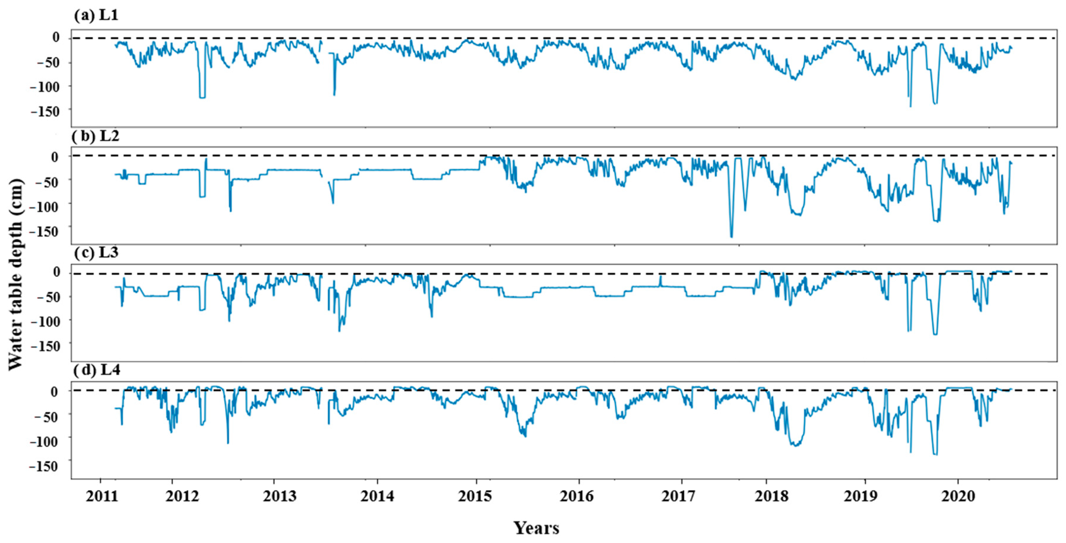
L10–14Sandy loam−2.4 to −160
14–44Sandy loam
44–63Sandy loam
63–180Sand
L20–40Loam−2.1 to −165
40–55Loamy sand
55–180Sand
L30–10Loam+4.7 to −130
10–27Loam
27–48Sandy loam
48–180Sand
L40–21Sandy loam+8.2 to −125
21–32Clay loam
32–56Sand
56–180Sand
Table 2. Leaf area index and above-ground biomass obtained from the initial simulations against the original data compared to the second series of simulations against normalised data.
Leaf Area IndexAbove-Ground Biomass
First SimSecond SimFirst SimSecond Sim
rRMSE0.470.461.550.90
d0.690.710.300.45
p-factor0.730.750.150.30
r-factor1.611.501.701.57
Disclaimer/Publisher’s Note: The statements, opinions and data contained in all publications are solely those of the individual author(s) and contributor(s) and not of MDPI and/or the editor(s). MDPI and/or the editor(s) disclaim responsibility for any injury to people or property resulting from any ideas, methods, instructions or products referred to in the content.

