
APEIOU Integration for Enhanced YOLOV7: Achieving Efficient Plant Disease Detection
Abstract
1. Introduction
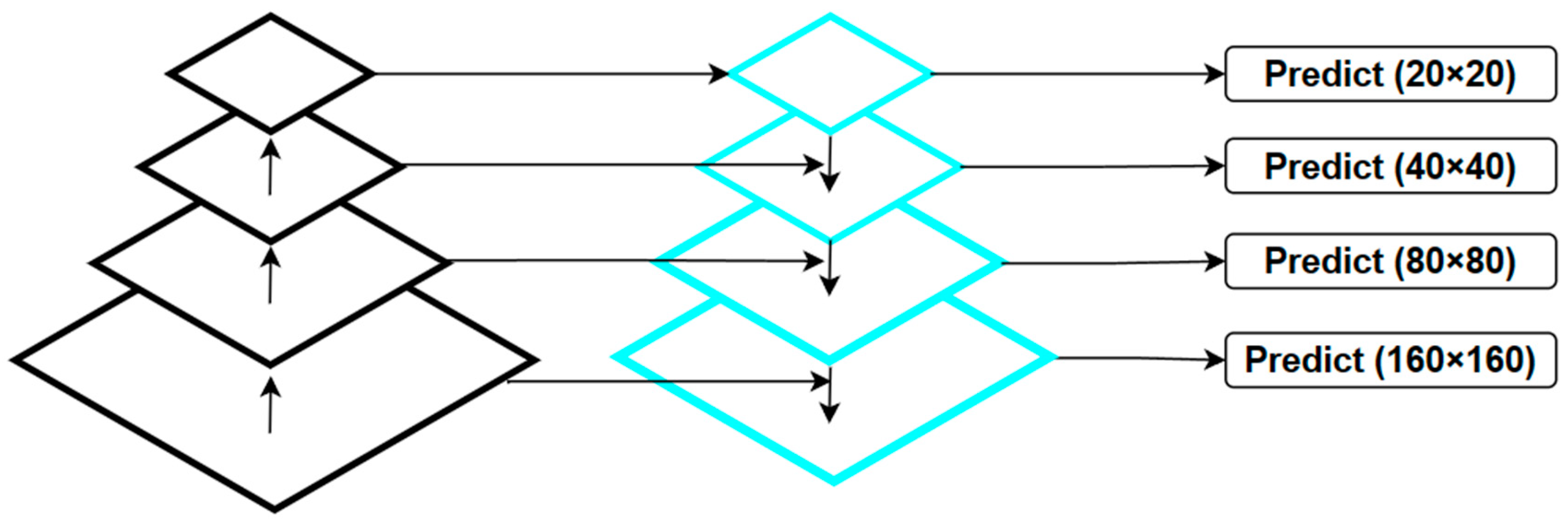
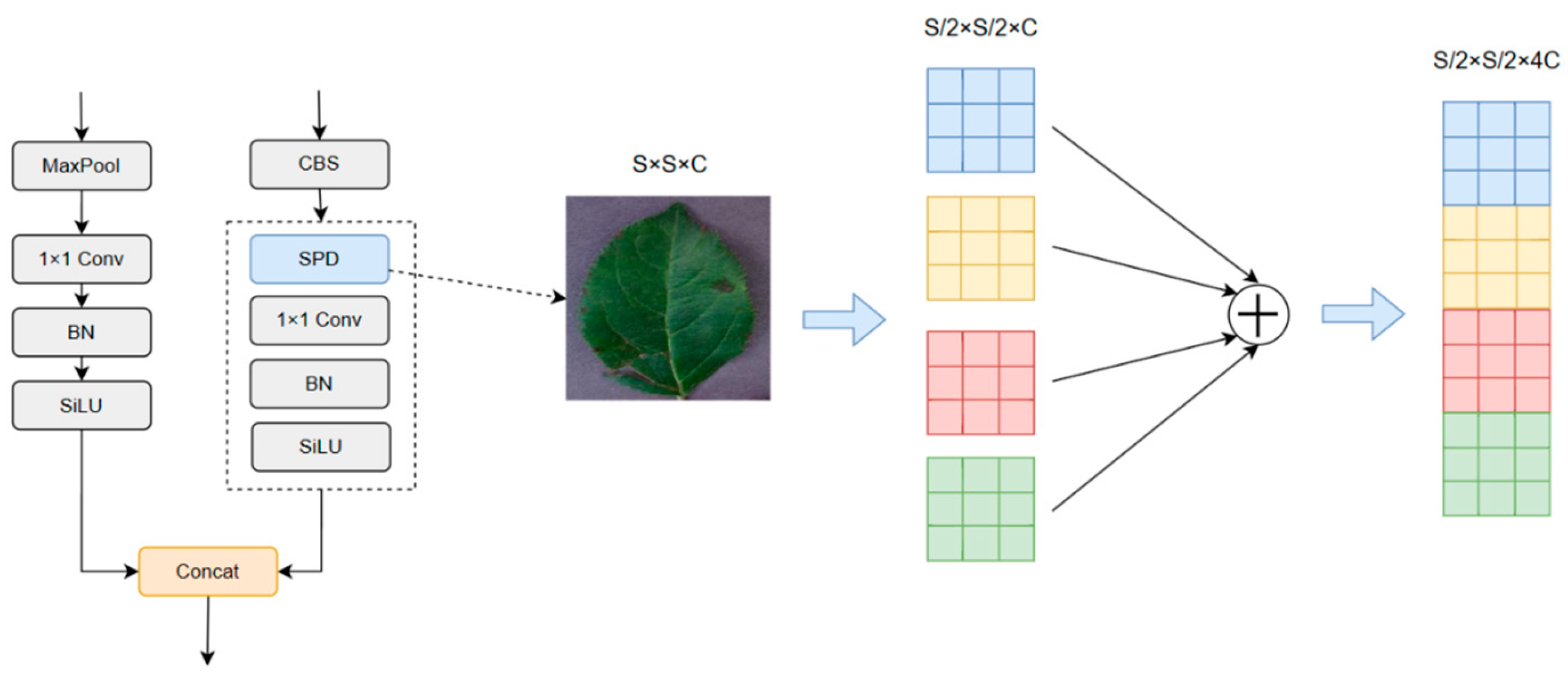
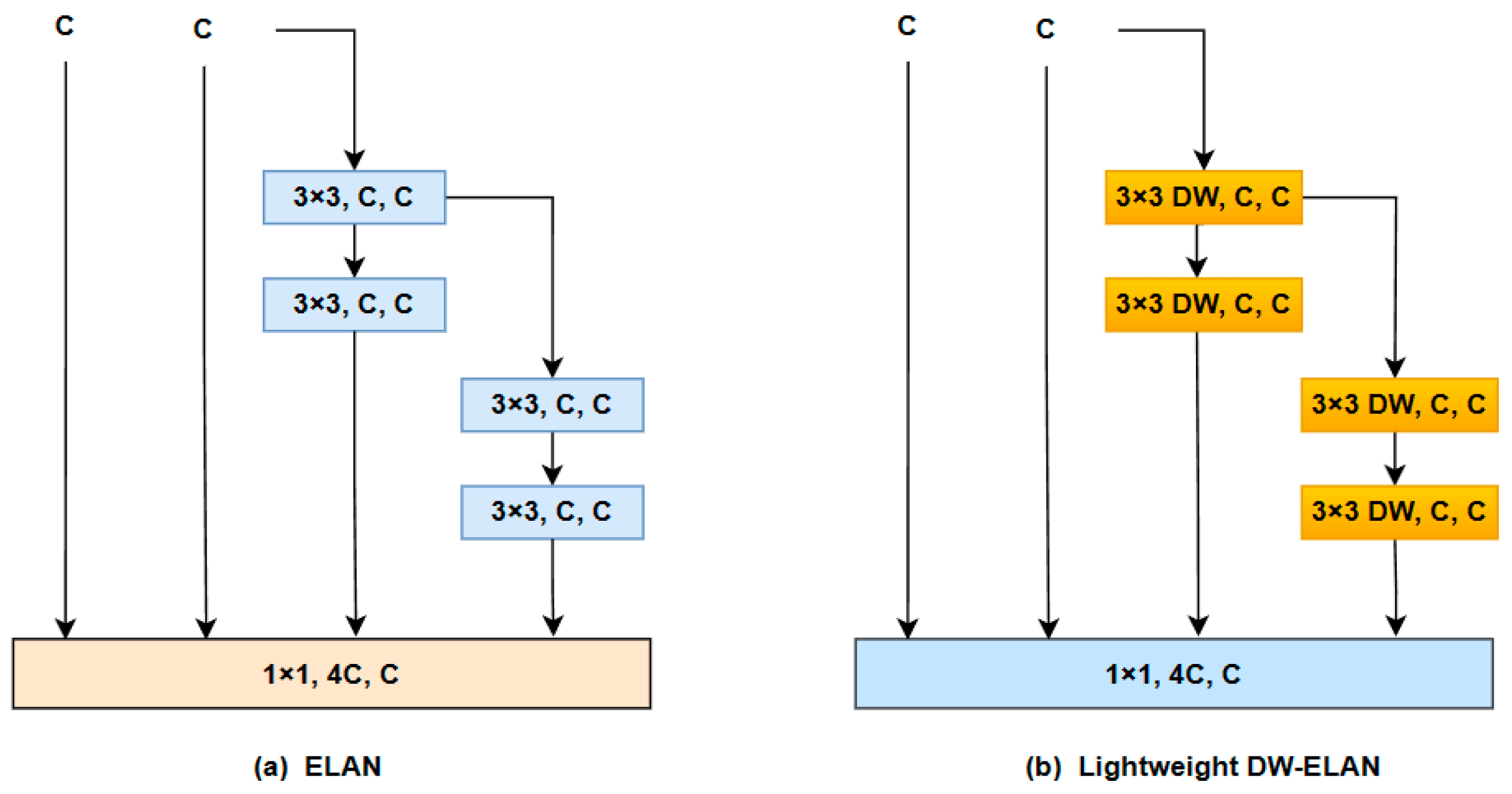
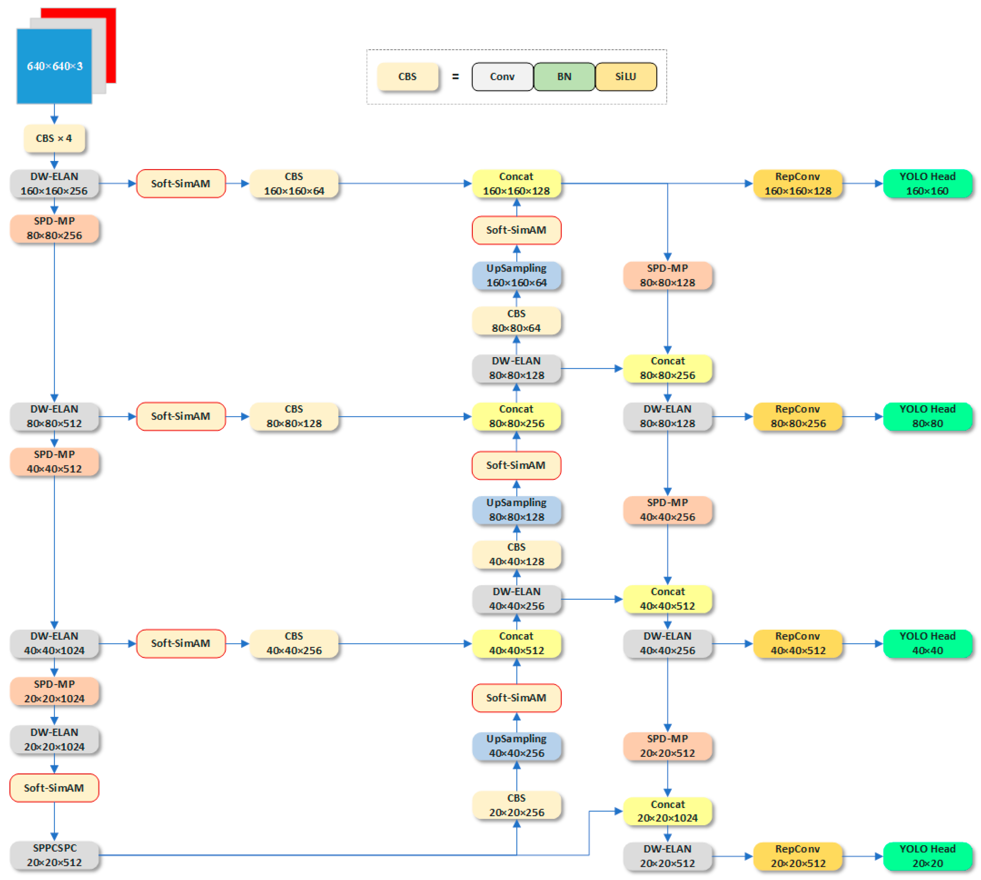
- We have enhanced the model structure of YOLO V7 to address the issue of increasing receptive fields during the downsampling process, which often leads to missing small objects. To mitigate this problem, we redesigned the fourth prediction head and proposed the SPD-MP structure to optimize the downsampling process in the backbone and neck sections. Additionally, we employed the lightweight DW-ELAN structure to achieve model lightweighting without significant performance loss.
- We introduced the improved lightweight attention mechanism, Soft-SimAM, during the backbone and upsampling stages. This mechanism enhances focus on high-weight regions while suppressing low-weight regions through the introduction of a softening threshold. As a result, feature maps before entering the fusion process pay more attention to detailed features.
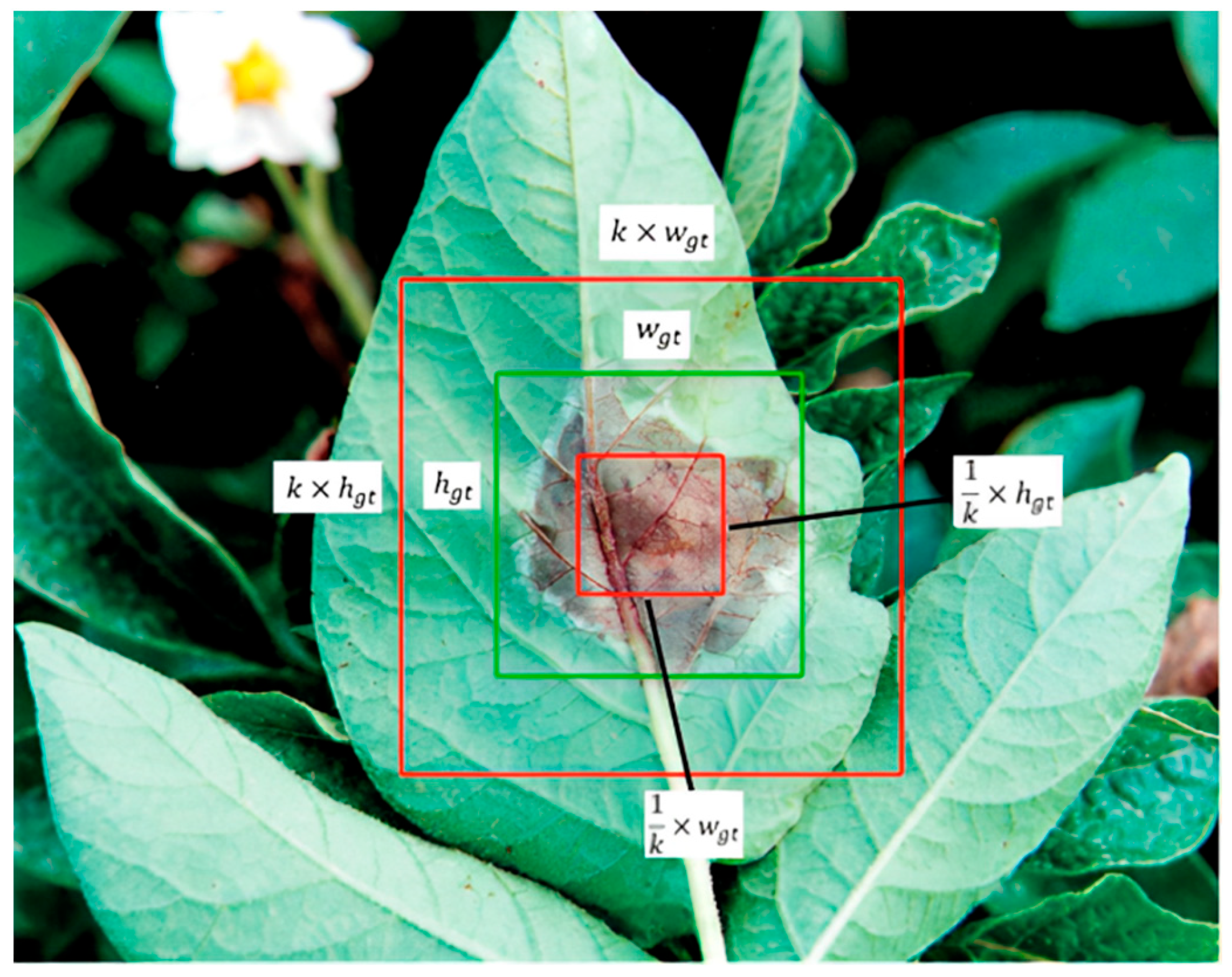
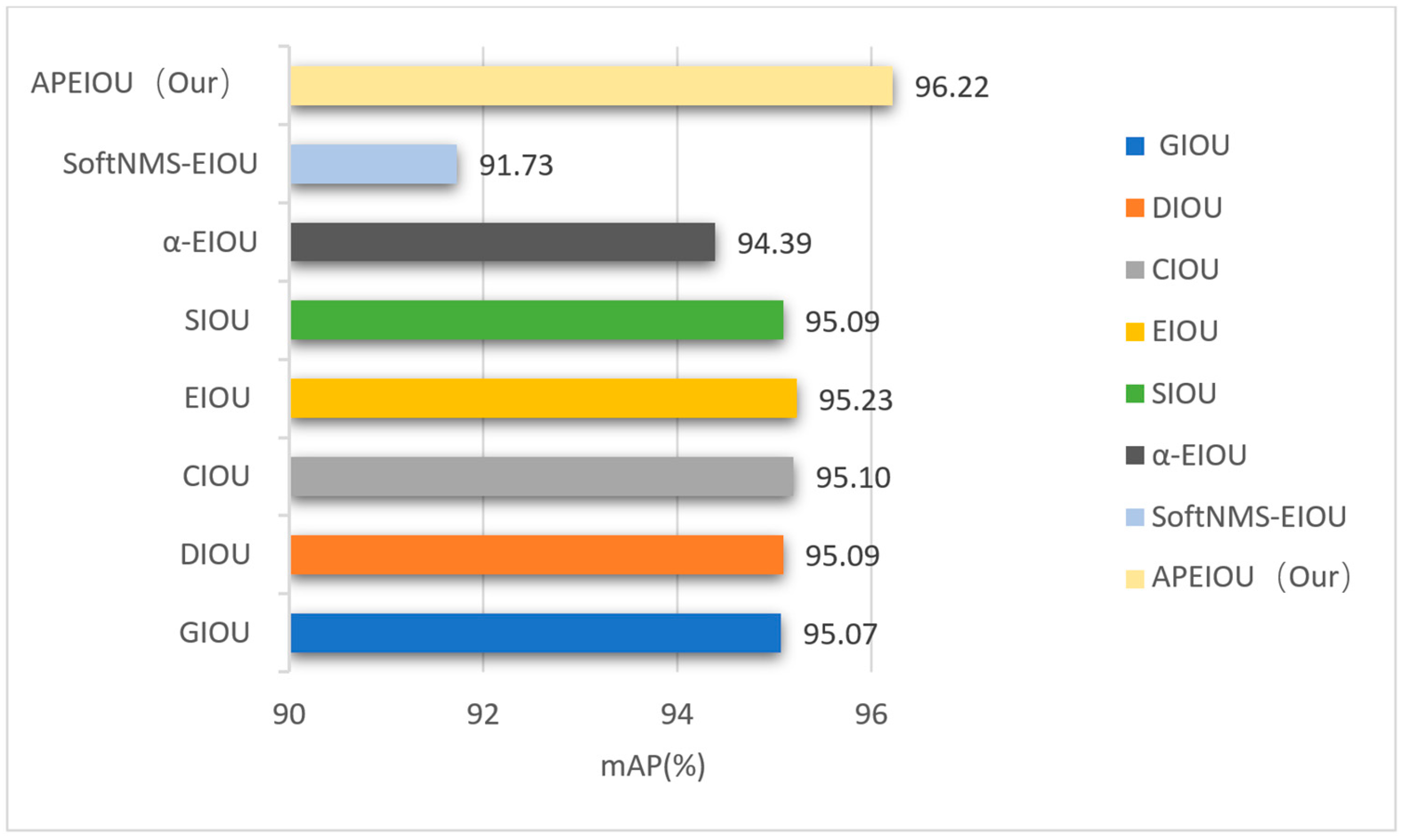
- We proposed APEIOU loss and designed an auxiliary penalty term to address situations where the predicted box and the ground truth box have the same aspect ratio but different width and height values, potentially resulting in identical loss values. This innovation aids in achieving higher precision in box regression.
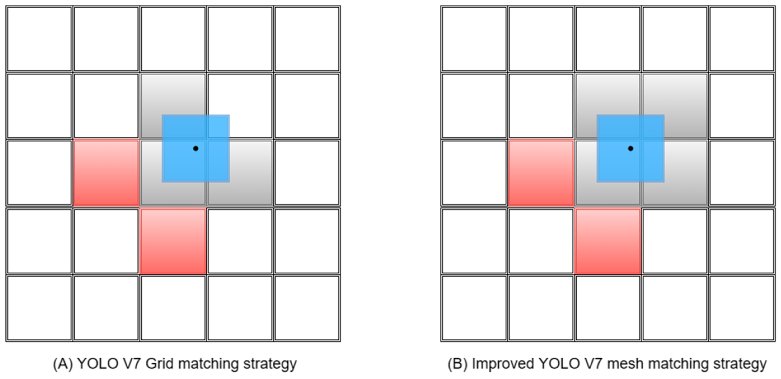
- We significantly increased the maximum number of positive samples that the lead head in YOLO V7 can match by adding prediction layers and increasing the number of grid cells matched with ground truth boxes. This enhancement provides more choices for the subsequent SimOTA fine screening. Additionally, we investigated the impact of the dynamic_k parameter on the training speed during the positive sample screening process in SimOTA under different settings.
2. Materials and Methods
2.1. Materials
2.1.1. Image Dataset
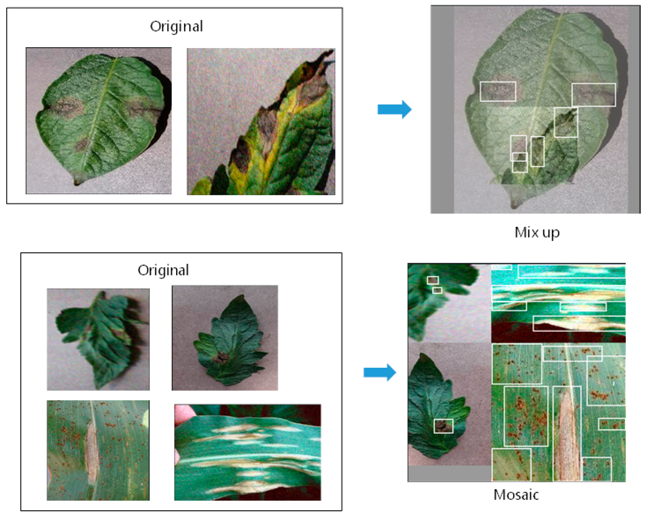
2.1.2. Image Augmentation
2.2. Methods
2.2.1. Improvement of the YOLO V7 Structure
2.2.2. Improvement of Attention Mechanism
2.2.3. Improvement of the Loss Function
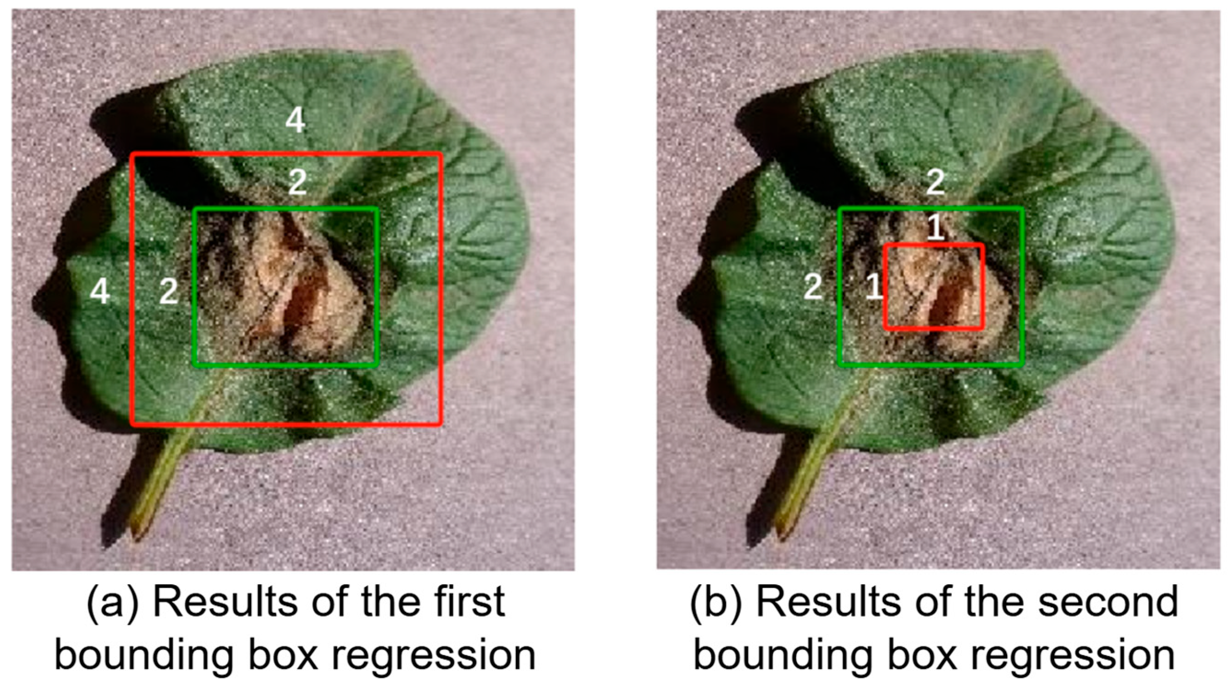
- predicted bounding boxes coincide with the center of the ground truth bounding box
- In the calculation of prediction box 2 versus the ground truth box:
- The following loss calculation is performed using the loss function proposed in this paper.
- In the calculation of prediction box 1 versus the ground truth box:
- In the calculation of prediction box 2 versus the ground truth box:
- .□
2.2.4. Improved Grid Matching Strategy
3. Results
3.1. Equipment Setting
3.1.1. Equipment and Experiment Parameter
3.1.2. Evaluation Metrics
3.2. Comparative Experiments and Deployment
3.2.1. Comparison of Different Attention Mechanisms
3.2.2. Comparative Experiments of Different Loss Functions
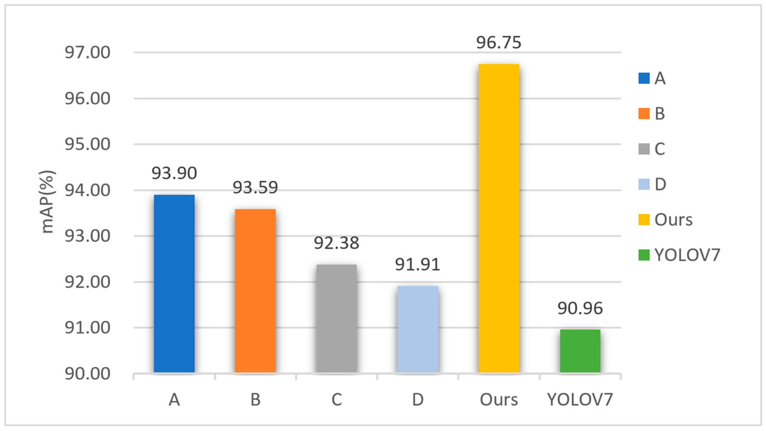
3.2.3. Comparative Experiments of Each Improvement Part
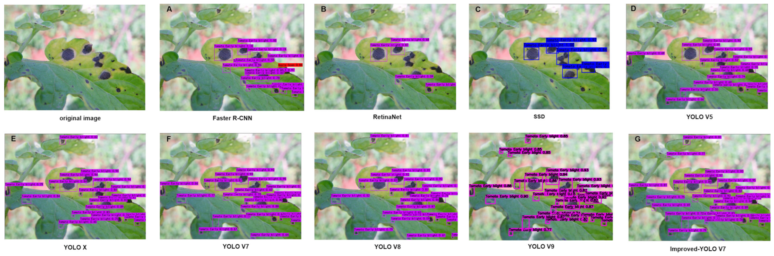
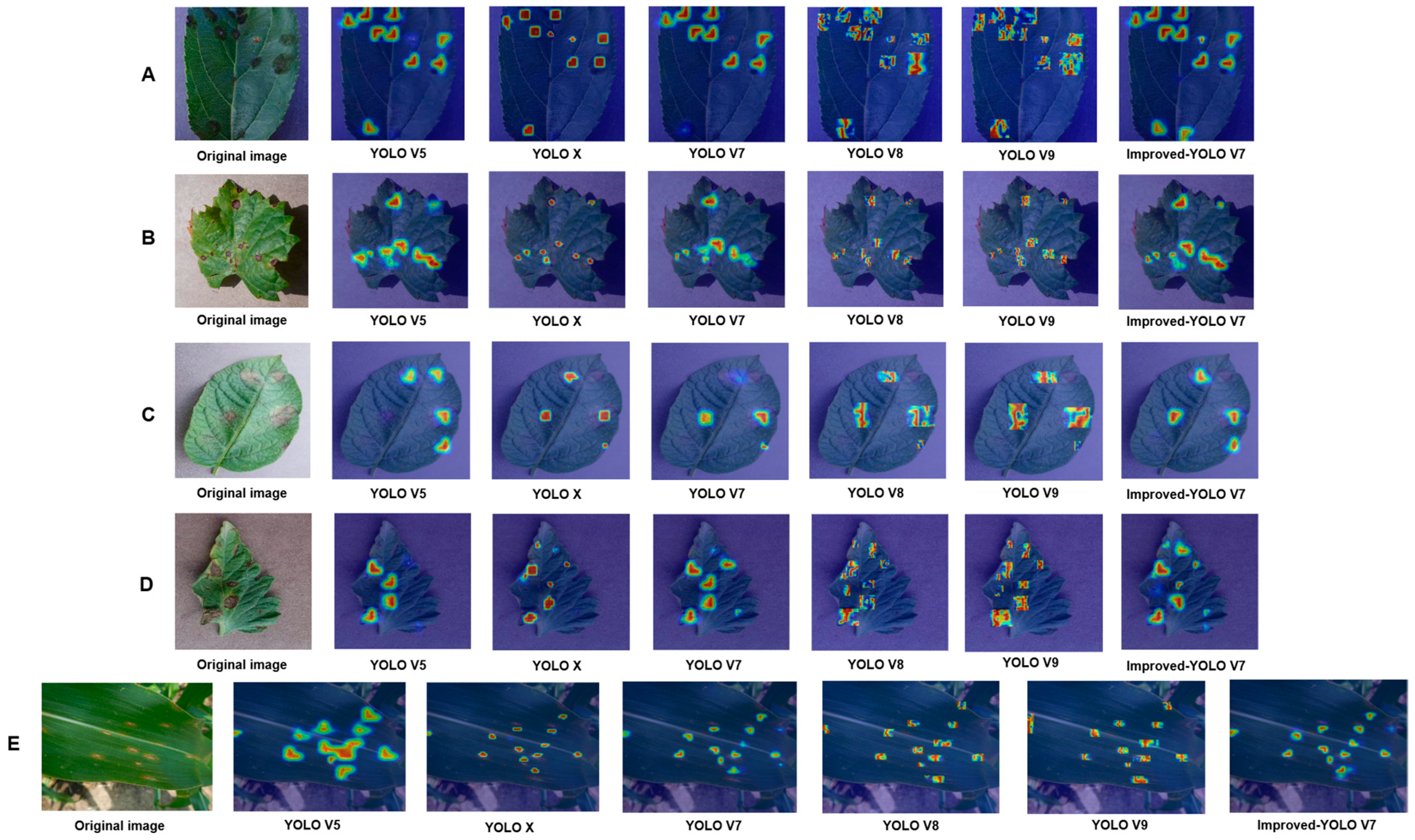
3.2.4. Comparative Experiments of Different Target Detection Models
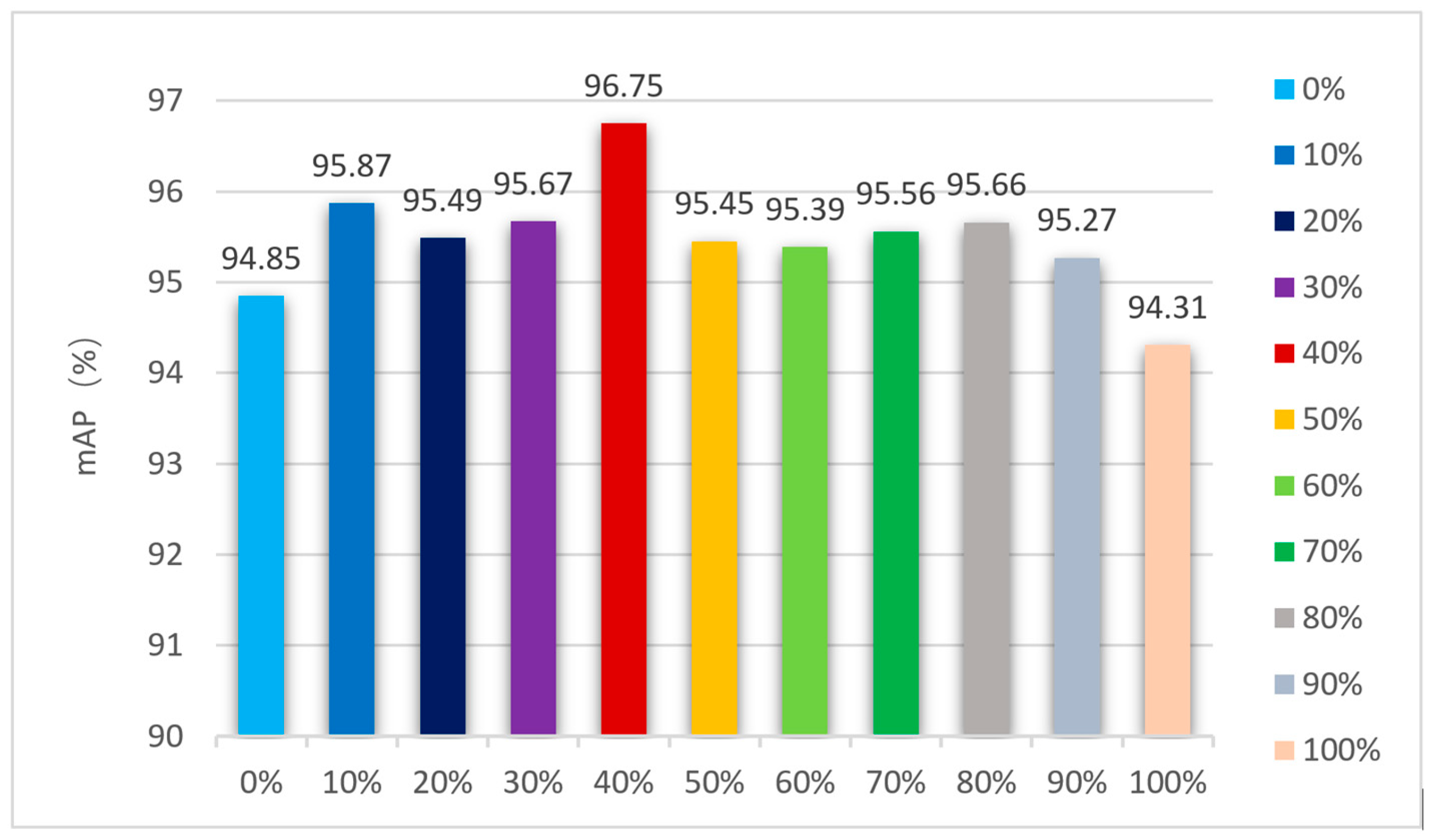
3.2.5. Comparison of Models under Different Anchors and Dynamic k Values
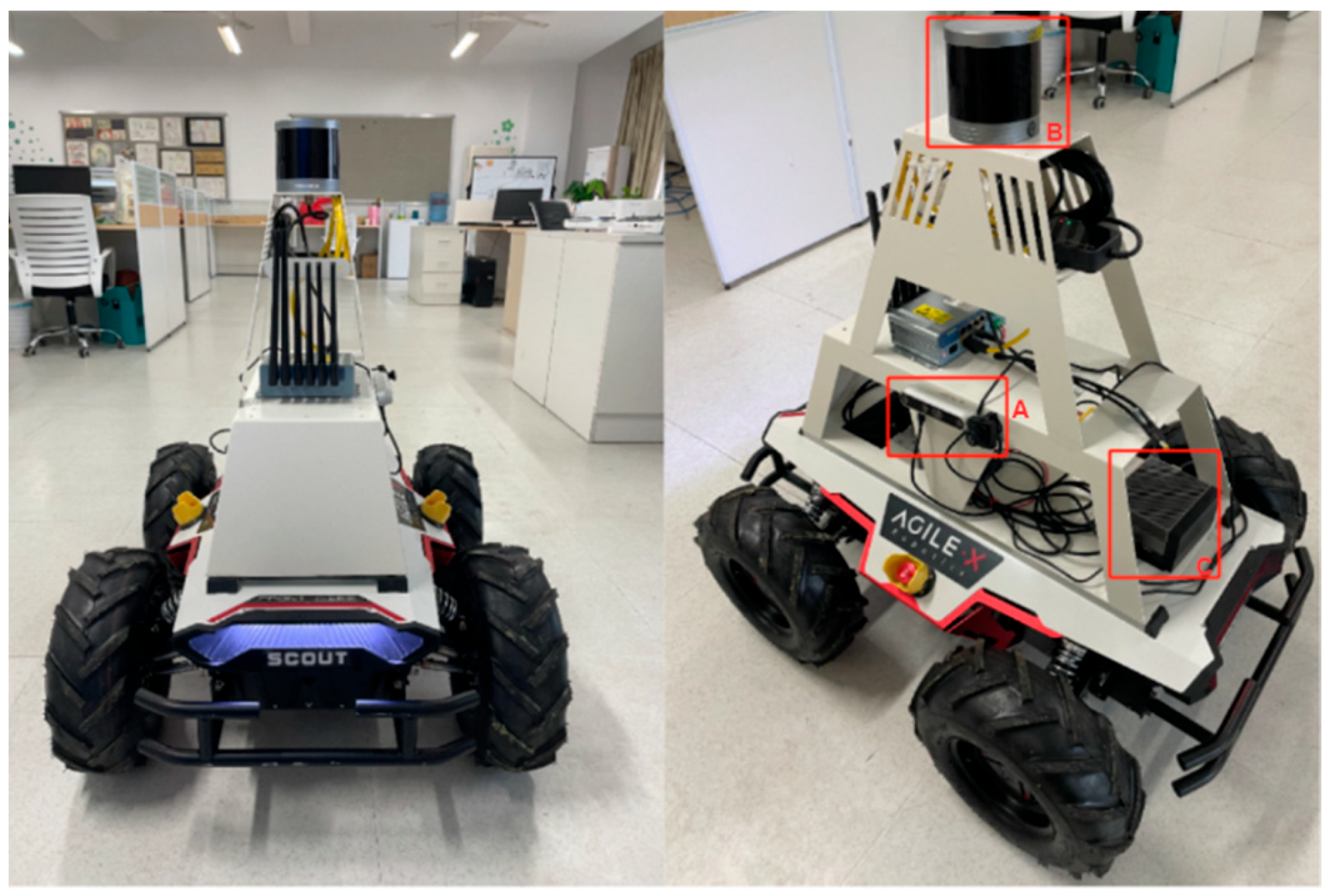
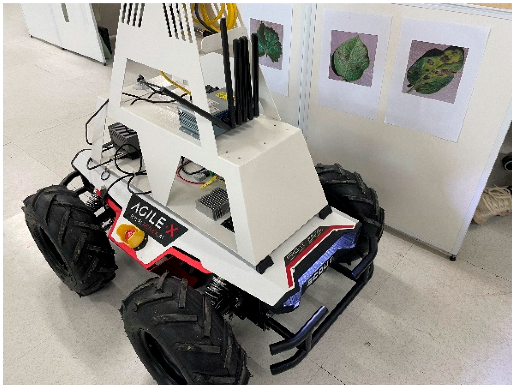
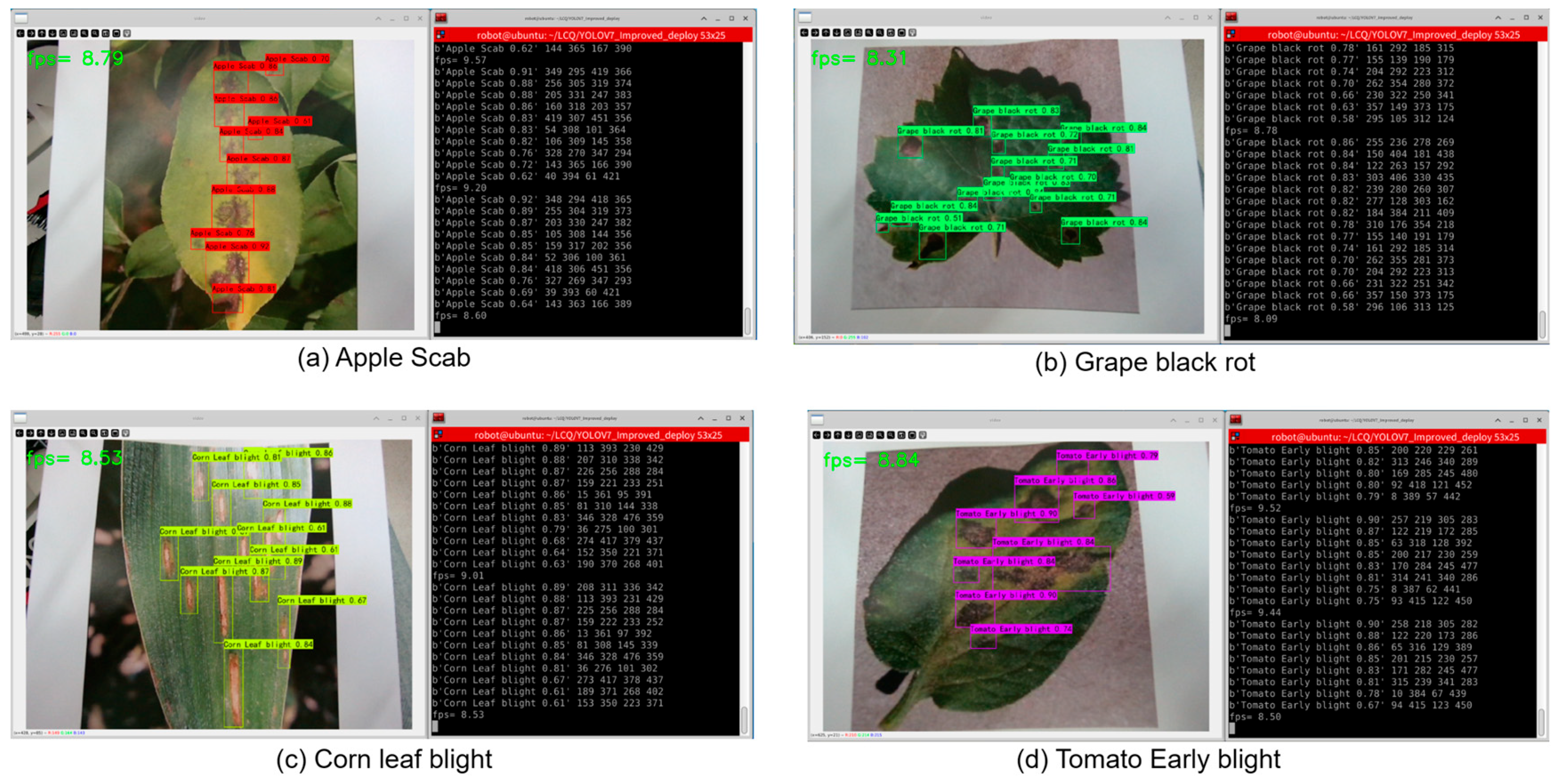
3.2.6. Deployment and Application
4. Discussion
5. Conclusions
Author Contributions
Funding
Institutional Review Board Statement
Data Availability Statement
Acknowledgments
Conflicts of Interest
References
- Sindhuja, S.; Ehsani, R.; Morganc, K.T. Detection of anomalies in citrus leaves using laser-induced breakdown spectroscopy (LIBS). Appl. Spectrosc. 2015, 69, 913–919. [Google Scholar]
- Parminder, K.; Pannu, H.S.; Malhi, A.K. Plant disease recognition using fractional-order Zernike moments and SVM classifier. Neural Comput. Appl. 2019, 31, 8749–8768. [Google Scholar]
- Kim, L.; Legay, A.; Nolte, G.; Schlüter, M.; Stoelinga, M. Formal methods meet machine learning (F3ML). In International Symposium on Leveraging Applications of Formal Methods; Springer Nature: Cham, Switzerland, 2022. [Google Scholar]
- Moez, K.; Mihoub, A.; Alzahrani, M.Y.; Adoni, W.Y.H.; Nahhal, T. Are formal methods applicable to machine learning and artificial intelligence? In Proceedings of the 2022 2nd International Conference of Smart Systems and Emerging Technologies (SMARTTECH), Riyadh, Saudi Arabia, 9–11 May 2022. [Google Scholar]
- Ross, G.; Donahue, J.; Darrell, T.; Malik, J. Rich feature hierarchies for accurate object detection and semantic segmentation. In Proceedings of the IEEE Conference on Computer Vision and Pattern Recognition, Columbus, OH, USA, 23–28 June 2014. [Google Scholar]
- Ross, G. Fast R-CNN. In Proceedings of the IEEE International Conference on Computer Vision, Santiago, Chile, 7–13 December 2015. [Google Scholar]
- Ren, S.; He, K.; Girshick, R.; Sun, J. Faster R-CNN: Towards real-time object detection with region proposal networks. arXiv 2015, arXiv:1506.01497. [Google Scholar] [CrossRef] [PubMed]
- Liu, W.; Anguelov, D.; Erhan, D.; Szegedy, C.; Reed, S.; Fu, C.-Y.; Berg, A.C. SSD: Single shot multibox detector. In Proceedings of the Computer Vision–ECCV 2016: 14th European Conference, Amsterdam, The Netherlands, 11–14 October 2016; Proceedings, Part I 14. Springer International Publishing: Cham, Switzerland, 2016. [Google Scholar]
- Lin, T.-Y.; Goyal, P.; Girshick, R.; He, K.; Dollár, P. Focal loss for dense object detection. In Proceedings of the IEEE International Conference on Computer Vision, Venice, Italy, 22–29 October 2017. [Google Scholar]
- Redmon, J.; Divvala, S.; Girshick, R.; Farhadi, A. You only look once: Unified, real-time object detection. In Proceedings of the IEEE Conference on Computer Vision and Pattern Recognition, Las Vegas, NV, USA, 27–30 June 2016. [Google Scholar]
- Redmon, J.; Farhadi, A. YOLO9000: Better, faster, stronger. In Proceedings of the IEEE Conference on Computer Vision and Pattern Recognition, Honolulu, HI, USA, 21–26 June 2017. [Google Scholar]
- Redmon, J.; Farhadi, A. Yolov3: An incremental improvement. arXiv 2018, arXiv:1804.02767. [Google Scholar]
- Bochkovskiy, A.; Wang, C.-Y.; Liao, H.-Y.M. Yolov4: Optimal speed and accuracy of object detection. arXiv 2020, arXiv:2004.10934. [Google Scholar]
- Ge, Z.; Liu, S.; Wang, F.; Li, Z.; Sun, J. Yolox: Exceeding yolo series in 2021. arXiv 2021, arXiv:2107.08430. [Google Scholar]
- Li, C.; Li, L.; Jiang, H.; Weng, K.; Geng, Y.; Li, L.; Ke, Z.; Li, Q.; Cheng, M.; Nie, W.; et al. YOLOv6: A single-stage object detection framework for industrial applications. arXiv 2022, arXiv:2209.02976. [Google Scholar]
- Wang, C.-Y.; Bochkovskiy, A.; Liao, H.-Y.M. YOLOv7: Trainable bag-of-freebies sets new state-of-the-art for real-time object detectors. In Proceedings of the IEEE/CVF Conference on Computer Vision and Pattern Recognition, Vancouver, BC, Canada, 17–24 June 2023. [Google Scholar]
- Wang, C.-Y.; Yeh, I.-H.; Liao, H.-Y.M. YOLOv9: Learning What You Want to Learn Using Programmable Gradient Information. arXiv 2024, arXiv:2402.13616. [Google Scholar]
- Gong, X.; Zhang, S. A high-precision detection method of apple leaf diseases using improved faster R-CNN. Agriculture 2023, 13, 240. [Google Scholar] [CrossRef]
- Lee, S.-H.; Gao, G. A Study on Pine Larva Detection System Using Swin Transformer and Cascade R-CNN Hybrid Model. Appl. Sci. 2023, 13, 1330. [Google Scholar] [CrossRef]
- Tian, L.; Zhang, H.; Liu, B.; Zhang, J.; Duan, N.; Yuan, A.; Huo, Y. VMF-SSD: A Novel v-space based multi-scale feature fusion SSD for apple leaf disease detection. IEEE/ACM Trans. Comput. Biol. Bioinform. 2022, 20, 2016–2028. [Google Scholar] [CrossRef] [PubMed]
- Sankareshwaran, S.P.; Jayaraman, G.; Muthukumar, P.; Krishnan, A. Optimizing rice plant disease detection with crossover boosted artificial hummingbird algorithm based AX-RetinaNet. Environ. Monit. Assess. 2023, 195, 1070. [Google Scholar] [CrossRef] [PubMed]
- Xu, W.; Wang, R. ALAD-YOLO: An lightweight and accurate detector for apple leaf diseases. Front. Plant Sci. 2023, 14, 1204569. [Google Scholar] [CrossRef] [PubMed]
- Lin, J.; Yu, D.; Pan, R.; Cai, J.; Liu, J.; Zhang, L.; Wen, X.; Peng, X.; Cernava, T.; Oufensou, S.; et al. Improved YOLOX-Tiny network for detection of tobacco brown spot disease. Front. Plant Sci. 2023, 14, 1135105. [Google Scholar] [CrossRef] [PubMed]
- Tian, Y.; Wang, S.; Li, E.; Yang, G.; Liang, Z.; Tan, M. MD-YOLO: Multi-scale Dense YOLO for small target pest detection. Comput. Electron. Agric. 2023, 21, 108233. [Google Scholar] [CrossRef]
- Xu, W.; Xu, T.; Thomasson, J.A.; Chen, W.; Karthikeyan, R.; Tian, G.; Shi, Y.; Ji, C.; Su, Q. A lightweight SSV2-YOLO based model for detection of sugarcane aphids in unstructured natural environments. Comput. Electron. Agric. 2023, 211, 107961. [Google Scholar] [CrossRef]
- Solimani, F.; Angelo, C.; Giovanni, D.; Angelo, P.; Stephan, S.; Francesco, C.; Vito, R. Optimizing tomato plant phenotyping detection: Boosting YOLOv8 architecture to tackle data complexity. Comput. Electron. Agric. 2024, 218, 108728. [Google Scholar] [CrossRef]
- Yang, G.; Wang, J.; Nie, Z.; Yang, H.; Yu, S. A lightweight YOLOv8 tomato detection algorithm combining feature enhancement and attention. Agronomy 2023, 13, 1824. [Google Scholar] [CrossRef]
- Yu, J.; Jiang, Y.; Wang, Z.; Cao, Z.; Huang, T. Unitbox: An advanced object detection network. In Proceedings of the 24th ACM International Conference on Multimedia, Amsterdam, The Netherlands, 15–19 October 2016. [Google Scholar]
- Lachlan, T.-S.; Petersson, L. Improving object localization with fitness NMS and bounded IOU loss. In Proceedings of the IEEE Conference on Computer Vision and Pattern Recognition, Salt Lake City, UT, USA, 18–23 June 2018. [Google Scholar]
- Rezatofighi, H.; Tsoi, N.; Gwak, J.; Sadeghian, A.; Reid, I.; Savarese, S. Generalized intersection over union: A metric and a loss for bounding box regression. In Proceedings of the IEEE/CVF Conference on Computer Vision and Pattern Recognition, Long Beach, CA, USA, 15–20 June 2019. [Google Scholar]
- Zheng, Z.; Wang, P.; Liu, W.; Li, J.; Ye, R.; Ren, D. Distance-IOU loss: Faster and better learning for bounding box regression. In Proceedings of the AAAI conference on Artificial Intelligence, New York, NY, USA, 7–12 February 2020; Volume 34. [Google Scholar]
- Zhang, Y.-F.; Ren, W.; Zhang, Z.; Jia, Z.; Wang, L.; Tan, T. Focal and efficient IOU loss for accurate bounding box regression. Neurocomputing 2022, 506, 146–157. [Google Scholar] [CrossRef]
- David, H.; Salathé, M. An open access repository of images on plant health to enable the development of mobile disease diagnostics. arXiv 2015, arXiv:1511.08060. [Google Scholar]
- Singh, D.; Jain, N.; Jain, P.; Kayal, P.; Kumawat, S.; Batra, N. PlantDoc: A dataset for visual plant disease detection. In Proceedings of the 7th ACM IKDD CoDS and 25th COMAD, Hyderabad, India, 5–7 January 2020; pp. 249–253. [Google Scholar]
- Zhang, H.; Cisse, M.; Dauphin, Y.N.; Lopez-Paz, D. mixup: Beyond empirical risk minimization. arXiv 2017, arXiv:1710.09412. [Google Scholar]
- Sunkara, R.; Luo, T. No more strided convolutions or pooling: A new CNN building block for low-resolution images and small objects. In Joint European Conference on Machine Learning and Knowledge Discovery in Databases; Springer Nature: Cham, Switzerland, 2022. [Google Scholar]
- Zhao, M.; Zhong, S.; Fu, X.; Tang, B.; Pecht, M. Deep residual shrinkage networks for fault diagnosis. IEEE Trans. Ind. Inform. 2019, 16, 4681–4690. [Google Scholar] [CrossRef]
- Yang, L.; Zhang, R.-Y.; Li, L.; Xie, X. Simam: A simple, parameter-free attention module for convolutional neural networks. In Proceedings of the International Conference on Machine Learning, Virtual, 18–24 July 2021. [Google Scholar]
- Ma, S.; Yong, X. MPDIoU: A loss for efficient and accurate bounding box regression. arXiv 2023, arXiv:2307.07662. [Google Scholar]
- Hu, J.; Shen, L.; Sun, G. Squeeze-and-excitation networks. In Proceedings of the IEEE Conference on Computer Vision and Pattern Recognition, Salt Lake City, UT, USA, 18–23 June 2018. [Google Scholar]
- Woo, S.; Park, J.; Lee, J.-Y.; Kweon, I.S. CBAM: Convolutional block attention module. In Proceedings of the European Conference on Computer Vision (ECCV), Munich, Germany, 8–14 September 2018. [Google Scholar]
- Wang, Q.; Wu, B.; Zhu, P.; Li, P.; Zuo, W.; Hu, Q. ECA-Net: Efficient channel attention for deep convolutional neural networks. In Proceedings of the IEEE/CVF Conference on Computer Vision and Pattern Recognition, Seattle, WA, USA, 13–19 June 2020. [Google Scholar]
- Hou, Q.; Zhou, D.; Feng, J. Coordinate attention for efficient mobile network design. In Proceedings of the IEEE/CVF Conference on Computer Vision and Pattern Recognition, Nashville, TN, USA, 20–25 June 2021. [Google Scholar]
- Liu, Y.; Shao, Z.; Hoffmann, N. Global attention mechanism: Retain information to enhance channel-spatial interactions. arXiv 2021, arXiv:2112.05561. [Google Scholar]

| Type of Diseases | Number |
|---|---|
| Apple scab | 1000 |
| Corn leaf blight | 1000 |
| Grape black rot | 1000 |
| Potato late blight | 1000 |
| Tomato early blight | 1000 |
| Different Attention | mAP (%) | mAP (%) Small Obj. | Params (M) | FLOPs (G) |
|---|---|---|---|---|
| SE | 92.97 | 47.3 | 37.52 | 104.84 |
| CBAM | 92.39 | 46.7 | 37.82 | 104.85 |
| ECA | 92.61 | 47.0 | 37.21 | 104.84 |
| CA | 92.93 | 45.7 | 37.67 | 104.87 |
| GAMA | 93.24 | 46.5 | 37.22 | 104.85 |
| SimAM | 93.00 | 47.2 | 37.21 | 104.83 |
| Soft-SimAM (our) | 93.59 | 47.9 | 37.21 | 104.83 |
| Each Improvement Part | mAP (%) | mAP (%) Small Obj. | Params (M) | FLOPs (G) | FPS |
|---|---|---|---|---|---|
| YOLO V7 | 90.96 | 48.0 | 37.21 | 104.83 | 30.6 |
| YOLO V7_A | 93.90 | 53.1 | 26.35 | 74.24 | 30.1 |
| YOLO V7_B | 93.59 | 52.7 | 37.21 | 104.83 | 30.2 |
| YOLO V7_C | 92.38 | 51.7 | 37.21 | 104.83 | 30.8 |
| YOLO V7_D | 91.91 | 51.2 | 37.21 | 104.83 | 29.5 |
| Improved-YOLO V7 | 96.75 | 58.1 | 26.35 | 74.24 | 28.8 |
| Type of Diseases | Model | AP (%) | F1 Score | Recall (%) | Precision (%) |
|---|---|---|---|---|---|
| Apple scab | YOLO V7 | 89.12 | 0.84 | 79.96 | 91.31 |
| Improved-YOLO V7 | 96.12 | 0.92 | 87.68 | 95.9 | |
| Corn leaf blight | YOLO V7 | 84.59 | 0.76 | 64.76 | 91.9 |
| Improved-YOLO V7 | 95.48 | 0.91 | 85.36 | 97.18 | |
| Grape black rot | YOLO V7 | 92.3 | 0.9 | 85.32 | 95.23 |
| Improved-YOLO V7 | 98.62 | 0.97 | 95.35 | 97.71 | |
| Potato late blight | YOLO V7 | 96.43 | 0.96 | 94.32 | 97.3 |
| Improved-YOLO V7 | 98.31 | 0.98 | 96.07 | 99.1 | |
| Tomato early blight | YOLO V7 | 92.37 | 0.87 | 79.95 | 95.99 |
| Improved-YOLO V7 | 95.22 | 0.91 | 84.01 | 98.32 |
| Model | mAP (%) | mAP (%) Small obj. | Params (M) | FLOPs (G) | F1 | Recall (%) | Precision (%) |
|---|---|---|---|---|---|---|---|
| Faster R-CNN | 79.61 | 27.9 | 136.77 | 370.01 | 0.65 | 84.73 | 52.94 |
| RetinaNet | 85.21 | 43.9 | 55.40 | 201.16 | 0.83 | 74.40 | 94.17 |
| SSD | 80.96 | 32.4 | 26.28 | 62.80 | 0.71 | 59.69 | 92.44 |
| YOLO V5 | 92.34 | 47.6 | 46.65 | 114.30 | 0.86 | 79.50 | 95.23 |
| YOLO X | 95.80 | 55.7 | 54.15 | 155.38 | 0.92 | 89.58 | 95.21 |
| YOLO V7 | 90.96 | 48.0 | 37.21 | 104.83 | 0.87 | 80.26 | 94.34 |
| YOLO V8 | 95.82 | 58.0 | 25.85 | 79.07 | 0.93 | 89.61 | 96.63 |
| YOLO V9 | 97.06 | 58.6 | 25.44 | 102.8 | 0.94 | 90.20 | 96.91 |
| Improved-YOLO V7 | 96.75 | 58.1 | 26.35 | 74.24 | 0.94 | 89.69 | 97.64 |
| Dynamic k Minimum | mAP (%) | Train Time |
|---|---|---|
| min = 1 | 96.75% | 1 d 22 h 38 m |
| min = 2 | 96.95% | 2 d 19 h 21 m |
| min = 3 | 96.77% | 2 d 21 h 47 m |
| Different Anchor | mAP (%) |
|---|---|
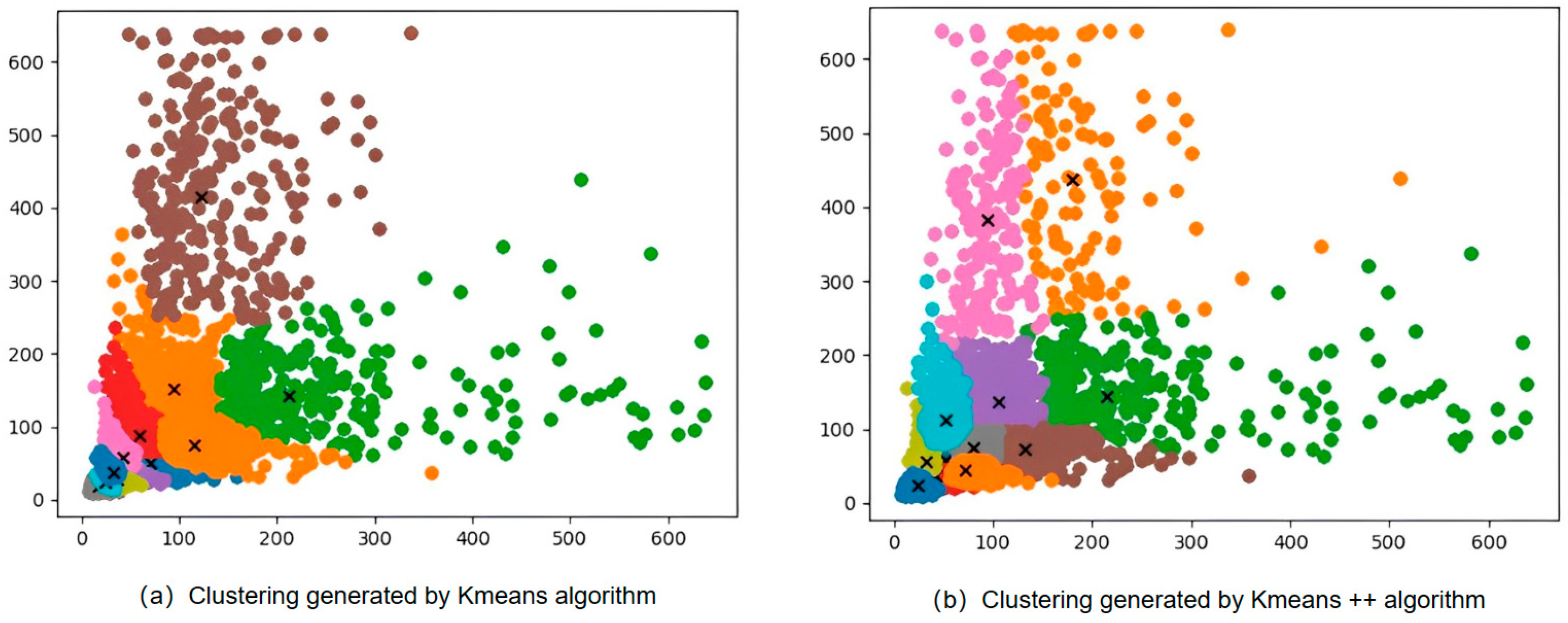
| Anchor generated by Kmeans | 96.75% |
| Anchor generated by Kmeans++ | 96.82% |
| Parameter Type | Parameter Value |
|---|---|
| Length, width, and height (mm) | 930 × 699 × 349 |
| Wheelbases (mm) | 498 |
| Front/Rear Wheelbase | 583 |
| Total weight | 67 ± 1 kg |
| Battery Type | li-ion battery |
| Battery parameters | 24 V 30 Ah |
| Power Drive Motor | DC brushless 4 × 400 W |
| Steering Forms | four-wheel differential steering |
| Major Parameter | Parameter Values |
|---|---|
| CPU | 12-core Arm Cortex-A78AE v8.2 64-bit processor (3 MB L2 + 6 MB L3) |
| GPU | 2048 NVIDIA CUDA cores and 64 Tensor cores @ 1 GHz |
| Memory | 32 GB 256-bit LPDDR5 @ 204.8 GB/s |
| Reservoir | 64 GB eMMC 5.1 |
| USB | 3× USB 3.2, 4× USB 2.0 |
| Vision accelerator | PVA v2.0 |
| Power mode | 15 W, 30 W or 50 W |
| Size | 100 × 87 mm |
Disclaimer/Publisher’s Note: The statements, opinions and data contained in all publications are solely those of the individual author(s) and contributor(s) and not of MDPI and/or the editor(s). MDPI and/or the editor(s) disclaim responsibility for any injury to people or property resulting from any ideas, methods, instructions or products referred to in the content. |
© 2024 by the authors. Licensee MDPI, Basel, Switzerland. This article is an open access article distributed under the terms and conditions of the Creative Commons Attribution (CC BY) license (https://creativecommons.org/licenses/by/4.0/).
Share and Cite
Zhao, Y.; Lin, C.; Wu, N.; Xu, X. APEIOU Integration for Enhanced YOLOV7: Achieving Efficient Plant Disease Detection. Agriculture 2024, 14, 820. https://doi.org/10.3390/agriculture14060820
Zhao Y, Lin C, Wu N, Xu X. APEIOU Integration for Enhanced YOLOV7: Achieving Efficient Plant Disease Detection. Agriculture. 2024; 14(6):820. https://doi.org/10.3390/agriculture14060820
Chicago/Turabian StyleZhao, Yun, Chengqiang Lin, Na Wu, and Xing Xu. 2024. "APEIOU Integration for Enhanced YOLOV7: Achieving Efficient Plant Disease Detection" Agriculture 14, no. 6: 820. https://doi.org/10.3390/agriculture14060820
APA StyleZhao, Y., Lin, C., Wu, N., & Xu, X. (2024). APEIOU Integration for Enhanced YOLOV7: Achieving Efficient Plant Disease Detection. Agriculture, 14(6), 820. https://doi.org/10.3390/agriculture14060820