Research and Experiment on Cruise Control of a Self-Propelled Electric Sprayer Chassis

Abstract

In order to address the issues of poor stability in vehicle speed and deteriorated spraying quality caused by changes in road slope and the decrease in overall mass due to liquid spraying, this study focuses on analyzing the structure and longitudinal dynamic characteristics of a 4WID high ground clearance self-propelled electric sprayer. By utilizing MATLAB/Simulink software, three subsystems, namely, the inverse longitudinal dynamics model, torque distribution model, and motor model, are established. The model takes into account the effects of longitudinal driving resistance, slope, and vehicle roll angle on the distribution of loads among the four wheels during slope driving. A seven-degrees-of-freedom dynamic model is developed. A hierarchical control structure is designed, incorporating an upper-level PID controller and a lower-level fuzzy PID controller, to control the overall system. The control algorithms are tailored to the specific characteristics of the sprayer’s operation, and simulation experiments are conducted under the corresponding operating conditions. Building upon this, a sensor-equipped experimental platform is set up in the self-propelled sprayer manufactured by the team in the preliminary stage. Real vehicle tests are conducted in two scenarios: transition transportation and field operations, with the evaluation of the overall vehicle speed serving as the performance metric to validate the correctness of the model and the control theory.

1. Introduction

As agricultural environmental protection requirements become increasingly stringent, electric-driven, high-clearance, self-propelled sprayers are poised to become a future trend. However, due to the complex working conditions of sprayers, changes in external road environments, and decreased curb weight caused by internal liquid spraying, issues such as poor driving speed stability, uneven spraying, and deteriorated work quality are prone to occur. Achieving cruise control of sprayers under disturbances in complex environments is a crucial means by which to enhance their operational quality and efficiency.

Currently, motion control and task control are the two core components of automatic control technology for intelligent agricultural machinery. Domestic and international scholars’ research on automatic agricultural machinery control primarily focuses on navigation path tracking control [1,2,3] and navigation positioning algorithms [4,5,6]. The study of constant-speed cruise control for agricultural machinery, as a crucial direction within motion control, presents more research opportunities compared to the study of adaptive cruise control for automobiles [7,8,9,10,11,12]. Most agricultural machinery studies target agricultural equipment powered by engines, adjusting the power system through parameters to achieve precise operational speeds [13,14]. Regarding agricultural machinery speed control, COEN et al. [15] developed a cruise control system based on a predictive controller designed using the harvester’s dynamic model, minimizing engine speed without compromising acceleration performance. KAYACAN et al. [16] controlled the longitudinal speed of tractors using a PID controller during the design of agricultural vehicles. Miao Zhonghua et al. [17] proposed a real-time adjustment algorithm for a cotton picker’s working speed based on fuzzy PID control, establishing a speed adjustment model to achieve optimal control of the cotton picker’s working speed. He Jie et al. [18] designed an expert PID speed control algorithm and PID interpolation mechanism control algorithm with a combined control strategy for rice transplanters, enabling automatic control of planting operations and speeds.

The spray machine cruise control is an automatic control strategy designed to maintain a constant speed of the spray machine during field operations. This control method is crucial for crop protection operations, as implementing cruise control for the spray machine can reduce human error and resource wastage, aiding farmers in accurately applying crop protection products. Based on their independently developed novel four-wheel-drive and steerable spray machine, the Shen Yue team [19] established the kinematic model of the chassis and adopted a hierarchical control approach. Through an upper-level wheel speed distribution controller and a lower-level wheel speed coordination controller for speed control, the results demonstrated that the maximum speed fluctuation controlled was 0.2 m/s, meeting the operational requirements of the spray machine.

In conclusion, there is a limited number of in-depth studies on the longitudinal velocity control of electric sprayers, with little consideration given to the unique operational characteristics of sprayers and external disturbances. Moreover, the majority of research relies on conventional PID algorithms, leading to issues concerning robustness and control precision balance. Therefore, this study, taking into account the structural features of high-clearance, self-propelled electric sprayers, aims to establish an accurate mathematical model under external disturbances and to implement a hierarchical control structure to investigate speed control strategies for constant-speed cruising. This approach seeks to achieve stable speed control during the operation of the sprayer, meeting the requirements for high-quality pesticide spraying. Subsequently, the real-time experimental platform for speed control during cruising is constructed for the sprayer, and experiments are conducted during transitional transport and field operations to validate the established model and control algorithms.

2. Materials and Methods

2.1. Test Platform Construction

The experimental platform was established based on a high-clearance, self-propelled sprayer constructed by our team. The chassis of the sprayer is a swing-type flexible electric chassis, with specific parameters outlined in

Table 1. Overall technical design parameters of sprayer chassis.

Parameter Name	Parameter Unit	Description
Chassis drive form	/	Four-wheel independent motor drive
Steering form	/	Four-wheel independent motor steering
Vehicle full load mass	kg	450
Sprayer wheelbase	mm	1200
Ground clearance	mm	600
Maximum working speed	km/h	20.0
Minimum working speed	km/h	3.0

.

A six-axis attitude measurement gyroscope module was installed at the center of gravity position of the sprayer to measure vehicle acceleration, speed, and body posture. The vehicle controller employed an IMC T3654 industrial programmable controller from Hirschmann, along with a remote controller featuring a human–machine interface, as depicted in Figure 1.

The selected IMC T3654 controller is based on a 32-bit Tricore platform, known for its fast response speed and high efficiency. It offers an open programming environment and a rich set of mature application modules. The control algorithm developed earlier can be converted into program code using Codesys and then burned into the controller (the version of the programming tool is Codesys v3.5 sp4).

The IMC T3654 controller is housed in the control box at the front of the sprayer. To measure the acceleration at the center of gravity, a JY61P six-axis attitude sensor is fixed to the support beam below the tank. By integrating the acceleration data, the current driving speed can be determined. Additionally, the sensor provides the vehicle’s pitch angle, allowing for the calculation of the current slope gradient. The final setup of the experimental vehicle platform is illustrated in Figure 2.

2.2. Analysis of the Overall Cruise Control Model Architecture

Dynamic models were established for each component of the chassis. In order to ensure the accuracy and conciseness of the longitudinal dynamic model and control system, a mechanistic analysis of each part of the system is conducted. Subsequently, a longitudinal dynamic simulation system for the sprayer is developed, and simulations are carried out using Simulink to validate the model’s correctness, facilitating the application of control algorithms on the model in the future.

The working environment of the sprayer is complex, with road conditions potentially varying between uphill and downhill slopes during operation. To analyze the longitudinal forces and motion states of the sprayer when driving on slopes, the force diagram is established in the spatial coordinate system as shown in Figure 3. The ground coordinate system is symbolized by X_s-Y_s-Z_s, with the directions of X_s, Y_s, and Z_s following the right-hand rule, and the coordinate origin O_s fixed at a corner of the slope. The coordinate system that moves with the center of mass of the sprayer’s spring-loaded mass is symbolized by X_v-Y_v-Z_v, with its origin O_v coinciding with the center of mass of the sprayer’s spring-loaded mass. When the sprayer travels on an inclined plane, the negative direction along the X_v axis represents its longitudinal motion, Y_v denotes the lateral direction, and Z_v indicates the vertical direction.

The slope angle is the angle between the projection of the slope on the Y_s-O_s-Z_s plane in the spatial coordinate system X_s-Y_s-Z_s and the Y_s axis. The heading angle of the sprayer when traveling on the slope is represented by θ, where θ is the angle between the velocity of the center of mass and the Y_s-O_s-Z_s plane in the spatial coordinate system. The body roll angle of the sprayer in the spatial coordinate system is represented by α, and the pitch angle is represented by β.

When establishing the longitudinal dynamic model of the sprayer, the following assumptions are made:

(1)

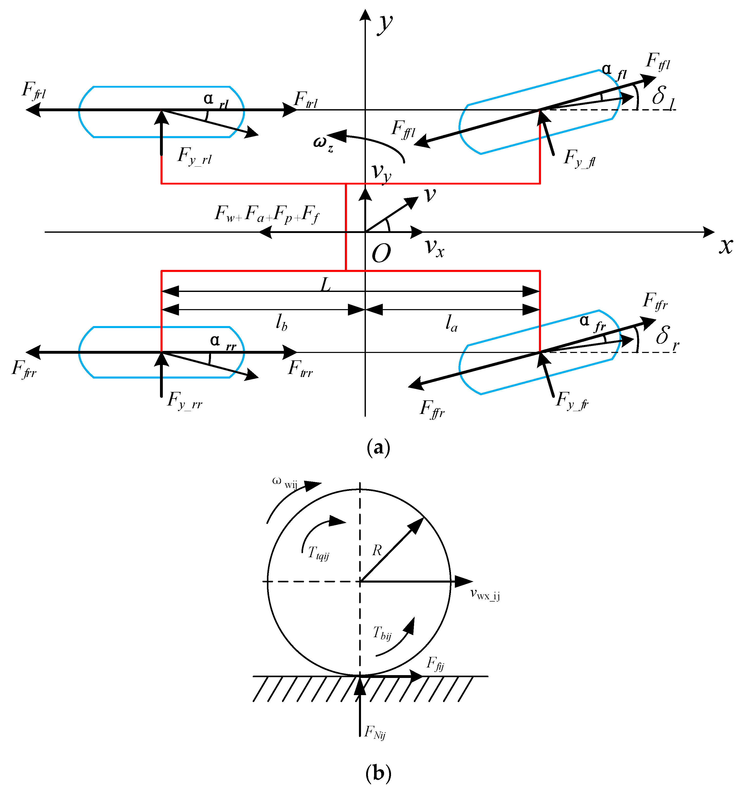
The deformation of the tires and the ground are neglected.

(2)

The entire body of the sprayer is symmetrical from left to right.

(3)

The tires are in a pure rolling state without side slip or slip, and the tire–road adhesion is ideal.

Based on the above assumptions, this paper considers the sprayer operating under slope conditions, establishing a longitudinal dynamic model with simultaneous pitch and roll of the vehicle body.

To analyze the longitudinal dynamic characteristics of the electric self-propelled sprayer, an electric sprayer’s longitudinal dynamic simulation system is first established. The system mainly consists of four parts, namely, an inverse longitudinal dynamic model, a torque distribution model, a motor model, and a seven-degrees-of-freedom vehicle body model, as shown in Figure 4.

a_des serves as the input to the inverse longitudinal dynamic model. After passing through the inverse longitudinal dynamic model, the desired torque T_des is output to the torque distribution model. The torque distribution model calculates the desired torque for each of the four wheels based on factors such as the current posture of the sprayer and the slope of the road. The actual torques are obtained through the motor model; and finally, the actual torques of the four wheels are input into the seven-degrees-of-freedom vehicle body model of the sprayer to calculate the actual vehicle speed and acceleration.

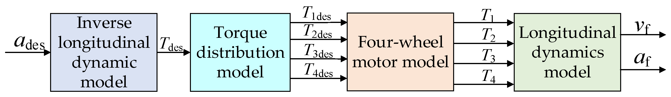
2.3. Modeling of Cruise Control Dynamics

2.3.1. Modeling of Inverse Longitudinal Dynamical Systems

According to Newton’s second law, the kinetic equation of the sprayer can be obtained as follows:

$$F_{\mathrm{t}}-F_{\mathrm{b}}=F_{\mathrm{w}}+F_{\mathrm{a}}+F_{\mathrm{p}}+F_{\mathrm{f}}.$$

(1)

In Equation (1), F_t is the total driving force of the sprayer, N; F_b is the braking force, N; and F_f is the rolling resistance, N.

The formula for each part of resistance is shown in Equation (2).

$$\{\begin{array}{l}{F}_{\mathrm{w}}=\frac{1}{2}{C}_{\mathrm{D}}A\rho V_{\mathrm{r}}^2=\frac{C_{\mathrm{D}}A{V_{\mathrm{r}}}^2}{21.15}\\ F_{\mathrm{a}}=\delta Ma\\ F_{\mathrm{p}}=Mg\sin \beta \cos \theta \\ F_{\mathrm{f}}=\mu Mg\cos \alpha \cos \beta \end{array}$$

(2)

In Equation (2), C_D is the air resistance coefficient; A is the windward area of the sprayer, m²; V_r is the traveling relative speed, m/s; V_r = V + V_wind, and considering the traveling of the sprayer under the windless condition, the relative speed at this time is the traveling speed of the sprayer; δ is the mass conversion factor that relates to the moment of inertia of the rotating parts of the sprayer, such as the wheels, and is usually greater than one [20]; a is the traveling acceleration of the sprayer, m/s²; and μ is the rolling resistance coefficient.

The equation for the longitudinal dynamics of the sprayer during acceleration can be expressed as follows:

$$Ma=F_{\mathrm{t}}-F_{\mathrm{b}}-F_{\mathrm{w}}-F_{\mathrm{a}}-F_{\mathrm{p}}-F_{\mathrm{f}}.$$

(3)

Furthermore, the total driving force of the sprayer is composed of the driving forces provided by the four in-wheel motors, respectively, as shown in Equation (4).

$$\{\begin{array}{l}{F}_{\mathrm{t}}=F_{\mathrm{tf}}+F_{\mathrm{tr}}\\ F_{\mathrm{tf}}=F_{\mathrm{tfl}}+F_{\mathrm{tfr}}\\ F_{\mathrm{tr}}=F_{\mathrm{trl}}+F_{\mathrm{trr}}\end{array}$$

(4)

In Equation (4), F_t is the driving force of the whole vehicle, N; F_tf and F_tr are the sum of the driving force of the front and rear axles of the sprayer, N; and F_tij is the driving force of each wheel individually (i = f,r; j = l,r), N, respectively.

The acting torque T_tqij of the hub motor on each wheel generates a circumferential force F₀ on the ground; and the reaction force F_tij of the ground on the wheel is the driving force of each wheel, expressed as follows:

$$F_{\mathrm{tij}}=\frac{T_{\mathrm{tqij}}{\eta }_{\mathrm{t}}}{R}.$$

(5)

In Equation (5), R is the rolling radius of the wheel, m; and η_t is the transmission efficiency of the in-wheel motor.

The sum of the output torque of the four hub motors can be calculated using Equations (2)–(5), jointly as follows:

$$T_{\mathrm{tq}}=\frac{R}{i_{\mathrm{g}}{\eta }_{\mathrm{t}}}\left\{\frac{C_{\mathrm{D}}A{V}^2}{21.15}+M\left[a\left(1+\delta \right)+g\sin \beta \cos \theta +\mu g\cos \alpha \cos \beta \right]\right\}.$$

(6)

2.3.2. Four-Wheel Torque Distribution Strategy

In the four-wheel drive mode of the sprayer, the overall vehicle driving torque, determined by the controller, needs to be appropriately distributed before it is transmitted to the four hub motors. This ensures efficient and energy-saving power output [21,22]. The distribution of the driving torques for each wheel of the sprayer during inclined slope conditions is based on the tire adhesion ratio. The tire adhesion ratio for each wheel during the sprayer’s movement on a slope can be expressed as follows [23]:

$$\{\begin{array}{l}{C}_{\mathsf{\phi }\mathrm{fl}}=\frac{F_{\mathrm{tfl}}}{F_{\mathrm{Nfl}}}\\ C_{\mathsf{\phi }\mathrm{fr}}=\frac{F_{\mathrm{tfr}}}{F_{\mathrm{Nfr}}}\\ C_{\mathsf{\phi }\mathrm{rl}}=\frac{F_{\mathrm{trl}}}{F_{\mathrm{Nrl}}}\\ C_{\mathsf{\phi }\mathrm{rr}}=\frac{F_{\mathrm{trr}}}{F_{\mathrm{Nrr}}}\end{array}.$$

(7)

In Equation (7), C_φfl, C_φfr, C_φrl, and C_φrr are the attachment rates of the left front wheel, right front wheel, left rear wheel, and right rear wheel, respectively; F_Nfl, F_Nfr, F_Nrl, and F_Nrr are the normal reaction forces of the ground on the left front wheel, right front wheel, left rear wheel, and right rear wheel, respectively, N.

When C_φfl = C_φfr = C_φrl = C_φrr, the driving forces of each wheel simultaneously reached the ground adhesion limit, and all the adhesion forces between the ground and the wheels could be converted into driving forces for the sprayer. Considering that the sprayer travels on a slope with both pitch and roll body states, the pitch angle and roll angle of the vehicle change with the direction of travel. Therefore, the normal reaction forces from the ground on each wheel vary, leading to a different distribution of driving forces for each wheel based on the varying normal reaction forces from the ground. Hence, the relationship for distributing the driving forces for each wheel can be determined as follows:

$$F_{\mathrm{tfl}}:F_{\mathrm{tfr}}:F_{\mathrm{trl}}:F_{\mathrm{trr}}=F_{\mathrm{Nfl}}:F_{\mathrm{Nfr}}:F_{\mathrm{Nrl}}:F_{\mathrm{Nrr}}.$$

(8)

Based on the longitudinal dynamics analysis of the sprayer in space, the longitudinal dynamic forces from the pitch and roll perspectives can be obtained. The sprayer model can be simplified into a two-wheel model, as shown in Figure 5.

The normal reaction forces on the front and rear wheels of the sprayer can be derived from the torque balance equation at the contact points with the ground. Similarly, the normal reaction forces on the left and right wheels of the sprayer can be obtained, as shown in Equation (9), based on the torque balance equation.

$$\{\begin{array}{l}{F}_{\mathrm{N}\_\mathrm{front}}=\frac{Mg(l_{\mathrm{b}}\cos \beta \cos \alpha -h\sin \beta )}{L}\\ F_{\mathrm{N}\_\mathrm{rear}}=\frac{Mg(l_{\mathrm{a}}\cos \alpha \cos \beta +h\sin \beta )}{L}\\ F_{\mathrm{N}\_\mathrm{left}}=\frac{Mg(h\sin \alpha +\frac{B}{2}\cos \alpha \cos \beta )}{B}\\ F_{\mathrm{N}\_\mathrm{right}}=\frac{Mg(\frac{B}{2}\cos \alpha \cos \beta -h\sin \alpha )}{B}\end{array}$$

(9)

The total vehicle normal support force and the torque distribution coefficients for each wheel of the sprayer can be obtained from Equation (9). Based on the torque distribution coefficients for each wheel of the sprayer, the optimal required torque for each wheel can be determined.

$$\{\begin{array}{l}{F}_{\mathrm{N}}=F_{\mathrm{N}\_\mathrm{front}}+F_{\mathrm{N}\_\mathrm{rear}}=F_{\mathrm{N}\_\mathrm{left}}+F_{\mathrm{N}\_\mathrm{right}}=M\mathrm{g}\cos \alpha \cos \beta \\ T_{\mathrm{tqfl}}={\psi }_{\mathrm{fl}}{T}_{\mathrm{tq}}=\frac{F_{\mathrm{N}\_\mathrm{front}}}{F_{\mathrm{N}}}\cdot \frac{F_{\mathrm{N}\_\mathrm{left}}}{F_{\mathrm{N}}}\cdot T_{\mathrm{tq}}\\ T_{\mathrm{tqfr}}={\psi }_{\mathrm{fr}}{T}_{\mathrm{tq}}=\frac{F_{\mathrm{N}\_\mathrm{front}}}{F_{\mathrm{N}}}\cdot \frac{F_{\mathrm{N}\_\mathrm{right}}}{F_{\mathrm{N}}}\cdot T_{\mathrm{tq}}\\ T_{\mathrm{tqrl}}={\psi }_{\mathrm{rl}}{T}_{\mathrm{tq}}=\frac{F_{\mathrm{N}\_\mathrm{rear}}}{F_{\mathrm{N}}}\cdot \frac{F_{\mathrm{N}\_\mathrm{left}}}{F_{\mathrm{N}}}\cdot T_{\mathrm{tq}}\\ T_{\mathrm{tqrr}}={\psi }_{\mathrm{rr}}{T}_{\mathrm{tq}}=\frac{F_{\mathrm{N}\_\mathrm{rear}}}{F_{\mathrm{N}}}\cdot \frac{F_{\mathrm{N}\_\mathrm{right}}}{F_{\mathrm{N}}}\cdot T_{\mathrm{tq}}\end{array}$$

(10)

Equation (10) defines ψ_fl, ψ_fr, ψ_rl, and ψ_rr as the torque distribution coefficients for the front left, front right, rear left, and rear right wheels of the sprayer, respectively.

2.3.3. Modeling of Motor Systems

The parameters of the selected hub motor were determined to have a maximum power of 953.05 W and a maximum torque of 80.34 N·m. By calculations, the rated speed of the hub motor was found to be 113.2889 r/min. Based on the generated external characteristic curve of the hub motor (as shown in Figure 6a) and its actual parameters, the drive motor model was established in MATLAB/Simulink (as shown in Figure 6b).

The motor is modeled in Simulink using the Lookup Table module according to the external characteristic curve of the motor. Meanwhile, in order to make the motor model conform to the reality, the following rules of torque output of the motor model are stipulated: according to the current speed of the motor, check the external characteristic table to obtain the maximum actual permissible torque; if the current demand torque is less than the maximum permissible torque, then the demand torque is output; if the current demand torque is more than the maximum permissible torque, then the output torque will be limited to the maximum permissible torque, which ensures the accuracy of the motor model.

2.3.4. Chassis Dynamics Modeling

The essence of vehicle modeling and stability analysis lies in accurately depicting the operational state of the vehicle, laying a solid foundation for vehicle control [24,25,26,27]. Given the focus of this study on speed sustainment control during the operation of the sprayer, particular attention should be paid to the sprayer’s motion characteristics in the horizontal plane during the dynamics analysis of the sprayer.

The schematic diagram of the chassis dynamic model of the sprayer is illustrated in Figure 7a,b, depicting a seven-degrees-of-freedom model and a wheel model. The seven-degrees-of-freedom model primarily encompasses the motion of the sprayer around the x-axis, y-axis, z-axis, and the rotational motion of the four wheels [28]. Therefore, considering the analysis presented earlier, the motion differential equations accounting for the driving resistance of the sprayer, the vertical forces on each tire, and the dynamics of the wheels can be expressed as Equation (11).

$$\{\begin{array}{l}M\left({\dot{\nu }}_{\mathrm{x}}-{\nu }_{\mathrm{y}}{\omega }_{\mathrm{z}}\right)=F_{\mathrm{tfl}}\cos {\delta }_{\mathrm{l}}+F_{\mathrm{tfr}}\cos {\delta }_{\mathrm{r}}-F_{\mathrm{y}\_\mathrm{fl}}\sin {\delta }_{\mathrm{l}}-F_{\mathrm{y}\_\mathrm{fr}}\sin {\delta }_{\mathrm{r}}+F_{\mathrm{trl}}+F_{\mathrm{trr}}-\\ F_{\mathrm{w}}-F_{\mathrm{a}}-F_{\mathrm{p}}-F_{\mathrm{f}}\\ M\left({\dot{\nu }}_{\mathrm{y}}+{\nu }_{\mathrm{x}}{\omega }_{\mathrm{z}}\right)=F_{\mathrm{tfl}}\sin {\delta }_{\mathrm{l}}+F_{\mathrm{tfr}}\sin {\delta }_{\mathrm{r}}+F_{\mathrm{y}\_\mathrm{fl}}\cos {\delta }_{\mathrm{l}}+F_{\mathrm{y}\_\mathrm{fr}}\cos {\delta }_{\mathrm{r}}+F_{\mathrm{y}\_\mathrm{rl}}+F_{\mathrm{y}\_\mathrm{rr}}\\ {\mathsf{{\rm I}}}_{\mathrm{z}}{\dot{\omega }}_{\mathrm{z}}=\frac{B_{\mathrm{f}}}{2}\left(F_{\mathrm{ffr}}\cos {\delta }_{\mathrm{r}}-F_{\mathrm{ffl}}\cos {\delta }_{\mathrm{l}}-F_{\mathrm{y}\_\mathrm{fr}}\sin {\delta }_{\mathrm{r}}+F_{\mathrm{y}\_\mathrm{f}l}\sin {\delta }_{\mathrm{l}}\right)+\frac{B_{\mathrm{r}}}{2}\left(F_{\mathrm{frr}}-F_{\mathrm{frl}}\right)\\ +l_{\mathrm{a}}\left(F_{\mathrm{ffl}}\sin {\delta }_{\mathrm{l}}+F_{\mathrm{y}\_\mathrm{fl}}\cos {\delta }_{\mathrm{l}}+F_{\mathrm{ffr}}\sin {\delta }_{\mathrm{r}}+F_{\mathrm{y}\_\mathrm{fr}}\cos {\delta }_{\mathrm{r}}\right)-l_{\mathrm{b}}\left(F_{{\mathrm{y}}_{\mathrm{rl}}}+F_{{\mathrm{y}}_{\mathrm{rr}}}\right)\\ F_{\mathrm{z}\_\mathrm{fl}}=m_{\mathrm{w}}g+\frac{Mg{l}_{\mathrm{b}}}{2L}\cos \beta -\frac{Mh{a}_{\mathrm{x}}}{2L}-\frac{Mh{a}_{\mathrm{y}}}{2B_{\mathrm{f}}}-\frac{Mgh\tan \alpha }{2B_{\mathrm{f}}}\\ F_{\mathrm{z}\_\mathrm{fr}}=m_{\mathrm{w}}g+\frac{Mg{l}_{\mathrm{b}}}{2L}\cos \beta -\frac{Mh{a}_{\mathrm{x}}}{2L}+\frac{Mh{a}_{\mathrm{y}}}{2B_{\mathrm{f}}}+\frac{Mgh\tan \alpha }{2B_{\mathrm{f}}}\\ F_{\mathrm{z}\_\mathrm{rl}}=m_{\mathrm{w}}g+\frac{Mg{l}_{\mathrm{a}}}{2L}\cos \beta +\frac{Mh{a}_{\mathrm{x}}}{2L}-\frac{Mh{a}_{\mathrm{y}}}{2B_{\mathrm{r}}}-\frac{Mgh\tan \alpha }{2B_{\mathrm{r}}}\\ F_{\mathrm{z}\_\mathrm{rr}}=m_{\mathrm{w}}g+\frac{Mg{l}_{\mathrm{a}}}{2L}\cos \beta +\frac{Mh{a}_{\mathrm{x}}}{2L}+\frac{Mh{a}_{\mathrm{y}}}{2B_{\mathrm{r}}}+\frac{Mgh\tan \alpha }{2B_{\mathrm{r}}}\\ I_{\mathrm{wij}}{\omega }_{\mathrm{wij}}=T_{\mathrm{tqij}}-F_{\mathrm{fij}}R-T_{\mathrm{bij}}\end{array}$$

(11)

In Equation (11), the longitudinal forces on the four wheels are represented by F_ffl, F_ffr, F_fr, and F_frr, N; the lateral forces on the four wheels are represented by F_{y_fl}, F_{y_fr}, F_{y_rl}, and F_{y_rr}, N; δ_l indicates the steering angle of the left front wheel, while δ_r represents the steering angle of the right front wheel, °; I_z stands for the moment of inertia of the sprayer around the z-axis, kg·m²; B_f corresponds to the front wheelbase distance, and B_r to the rear wheelbase distance, m; m_w denotes the weight of the tires, kg; a_x signifies the longitudinal acceleration of the sprayer in the x-direction, m/s², and a_y describes the lateral acceleration of the sprayer in the y-direction, m/s²; I_wij represents the moment of inertia of the wheel about the center of the hub motor, kg·m²; R is the wheel radius, m; and T_bij denotes the rolling resistance torque, N·m, where T_tqij provides driving torque when positive and acts as braking torque when negative.

To obtain accurate tire characteristics, suitable tire models must be established based on the specific research context to accurately describe the kinematic behavior of the tires, thereby enhancing the overall reliability and precision of the study [29,30]. Currently, in practical engineering studies, there exist various tire models, categorized as theoretical models, empirical models, semi-empirical models, and adaptive models [31,32,33].

Among these, the “magic formula” tire model proposed by H. B. Pacejka stands out as a typical empirical model known for its unified and concise form, offering high fitting accuracy [34,35]. This paper adopts the “magic formula” tire model, which employs a set of uniformly structured equations to precisely describe crucial mechanical properties such as longitudinal forces, lateral forces, and the aligning moments of the tire [36].

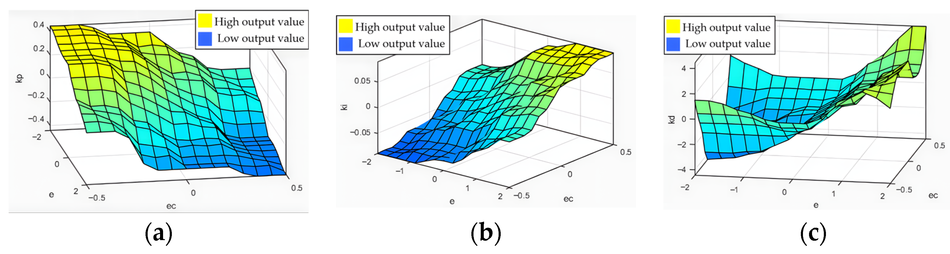
2.4. Design of Constant Speed Cruise Control Method Based on Fuzzy PID

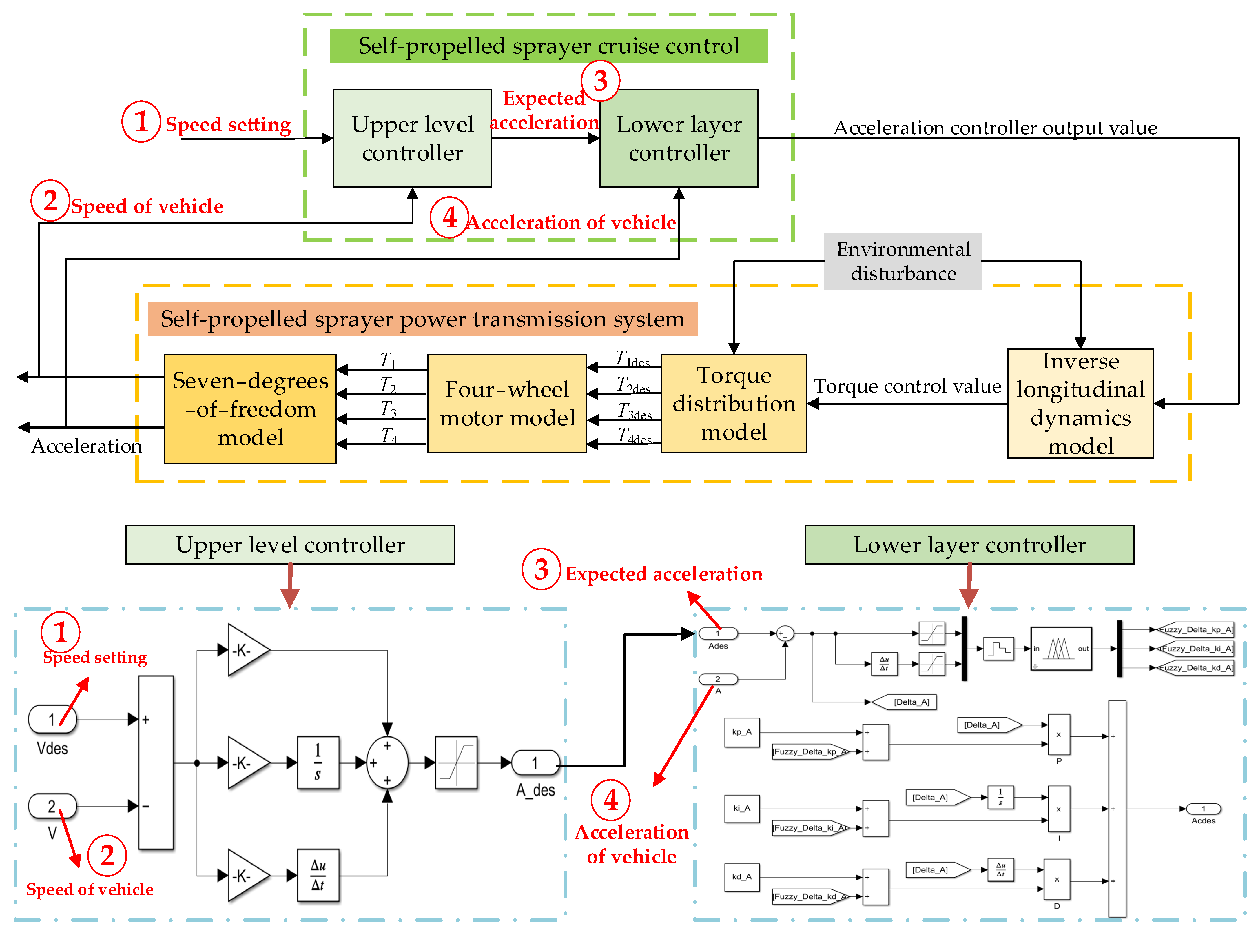
2.4.1. General Architecture of Cruise Control System for Self-Propelled Sprayers

The designed cruise control system in this study adopts a hierarchical control framework, consisting primarily of an upper-level controller and a lower-level controller. The upper-level controller is responsible for computing and determining the desired acceleration of the sprayer, while the lower-level controller, based on directives from the upper-level controller and actual acceleration values of the sprayer, outputs real control values to the dynamic model. The overall vehicle inverse longitudinal dynamics model and torque distribution model dynamically calculate the driving motor output torque in real time based on signals provided by the lower-level controller to ensure that the seven−degrees−of−freedom model tracks the desired acceleration, ultimately maintaining a constant speed. The schematic overview of the spray machine’s cruise control system is depicted in Figure 8, based on the outlined analysis. The figure illustrates the control models of the upper and lower controllers in Simulink. Additionally, the closed-loop feedback control signals between the controllers and the spray machine’s dynamic model are represented by the numbers 1−4 in the figure.

2.4.2. Upper and Lower Level Controller Design

For the upper-level controller, the PID control algorithm was employed to ensure rapid response [37]. It takes the user’s speed setpoint and real-time vehicle speed as inputs and outputs the desired acceleration to the lower-level controller.

During the parameterization of the upper controller. Initially, the proportional gain (k_p) was set to 2, while both integral (k_i) and derivative (k_d) gains were set to 0. Observing the response characteristics of the output, k_p was continuously adjusted to ensure good system sensitivity, while k_i was adjusted to reduce overshoot. After multiple iterations, the optimal PID parameter combination was determined to be k_p = 15, k_i = 3.97, and k_d = 0.

To avoid the instability issues associated with conventional PID control [38], the fuzzy PID control approach was ultimately adopted for the lower-level controller design, considering the complex operating conditions of the sprayer during travel. This method ensures control accuracy while maintaining smooth driving.

The error between the target acceleration and the actual acceleration, represented by e, along with the rate of change of the error, e_c, are considered as fuzzy values for the proportional (K_p), integral (K_i), and derivative (K_d) coefficients. Based on the current operating conditions of the self-propelled sprayer, the fundamental domain for the error e between the target and actual accelerations is [−2, 2], while the domain for the error rate e_c is [−0.5, 0.5]. These variables (K_p, K_i, K_d, e_c, e) are divided into seven fuzzy sets each, represented as NB, NM, NS, ZO, PS, PM, and PB, indicating negative large, negative medium, negative small, zero, positive small, positive medium, and positive large, respectively. After determining the fuzzy sets and domains, membership functions were established for the fuzzy variables. For NB and PB, zmf and smf membership functions were utilized, while trimf membership functions were used for the others. The membership functions have a narrow range in the middle and wider ranges on the sides to ensure quick stability when errors are small.

Drawing from the extensive driving experience of traditional vehicle drivers and the operational characteristics of the sprayer under study, fuzzy rules were formulated, taking into account response time and overshoot. Overshoot impacts the smooth operation of the sprayer; due to the significant mass of liquid in the tank, excessive acceleration could lead to increased liquid agitation within the tank, compromising the safety of the sprayer during operation. The formulation of fuzzy rules is as follows.

When the absolute value of the acceleration deviation e is large, the system’s response speed becomes a primary consideration. To reduce the time required to reach the cruising speed, increasing the tuning parameters K_p and K_i can enhance the spray machine’s dynamics, thereby correcting the deviation more quickly. However, this action may prematurely put the system into a regulation state, thereby prolonging the entire adjustment process. Therefore, fine-tuning of the tuning parameter K_d is necessary to appropriately reduce its value in order to balance the system’s response speed and stability.

When the absolute value of the acceleration deviation e only slightly exceeds a certain range, a moderate increase in the proportional gain K_p can enhance the system’s sensitivity to deviations. Based on the rate of change of the deviation e_c, the integral gain K_i is adjusted accordingly to optimize the system’s dynamic performance. Simultaneously, to minimize the system’s overshoot and ensure the safe and stable operation of the spray machine, the derivative gain K_d can be moderately increased.

When the absolute value of the acceleration deviation e is relatively small, indicating that the actual operating speed of the spray machine is close to the user-set cruising speed, the controller needs to avoid excessive overshoot. At this point, maintaining K_p and K_i at a relatively moderate level is essential, while slightly increasing the value of K_d can aid the system in better suppressing overshoot.

Following a comprehensive analysis of the deviation between the expected and actual acceleration values, fuzzy PID control rules were established, as presented in

Table 2. Adjustment table for control rules of parameters K_p, K_i, and K_d.

e	ec
	NB	NM	NS	ZO	PS	PM	PB
NB	PB/NB/PS	PB/NB/NS	PM/NM/NB	PM/NM/NB	PS/NS/NB	ZO/ZO/NM	ZO/ZO/PS
NM	PB/NB/PS	PB/NB/NS	PM/NM/NB	PS/NS/NM	PS/NS/NM	ZO/ZO/NS	NS/ZO/ZO
NS	PM/NB/ZO	PM/NM/NS	PM/NS/NM	PS/NS/NM	ZO/ZO/NM	NS/PS/NS	NS/PS/ZO
ZO	PM/NM/ZO	PM/NM/NS	PS/NS/NS	ZO/ZO/NS	NS/PS/NS	NM/PM/NS	NM/PM/ZO
PS	PS/NM/ZO	PS/NS/ZO	ZO/ZO/ZO	NS/PS/ZO	NS/PS/ZO	NM/PM/ZO	NM/PB/ZO
PM	PS/ZO/PB	ZO/ZO/NS	NS/PS/NS	NM/PS/PS	NM/PM/PS	NM/PB/PS	NB/PB/PB
PB	ZO/ZO/PB	ZO/ZO/PM	NM/PS/PM	NM/PM/PM	NM/PM/PS	NB/PB/PS	NB/PB/PB

.

After entering the rules in the table one by one in the MATLAB fuzzy logic design module, the characteristic surface corresponding to the input and output variables obtained is shown in Figure 9.

Subsequently, the fuzzy values output by the fuzzy controller were defuzzified to obtain precise output quantities. In this study, centroid defuzzification using the area centroid method was implemented in the MATLAB Fuzzy Logic Toolbox to ensure smooth output control. Ultimately, a constant speed cruise control system for the sprayer was established in Simulink. The controller takes the acceleration deviation and the rate of deviation as inputs and outputs K_p, K_i, and K_d. These three parameters are added to the proportional, integral, and derivative gains of the system in a simple PID control. The resulting value, after proportional, integral, and derivative operations on the deviation, is then summed to produce the acceleration control value for the sprayer. After tuning, the optimal initial fuzzy PID parameters were determined to be k_p = 2.5, k_i = 2.8, and k_d = 0.01.

3. Analysis of Simulation and Field Test Results

3.1. Analysis of Simulation Test Results

The vehicle dynamics model and controller model established in MATLAB/Simulink 2023a will be integrated to obtain the overall model for the constant speed cruise control, as shown in Figure 10.

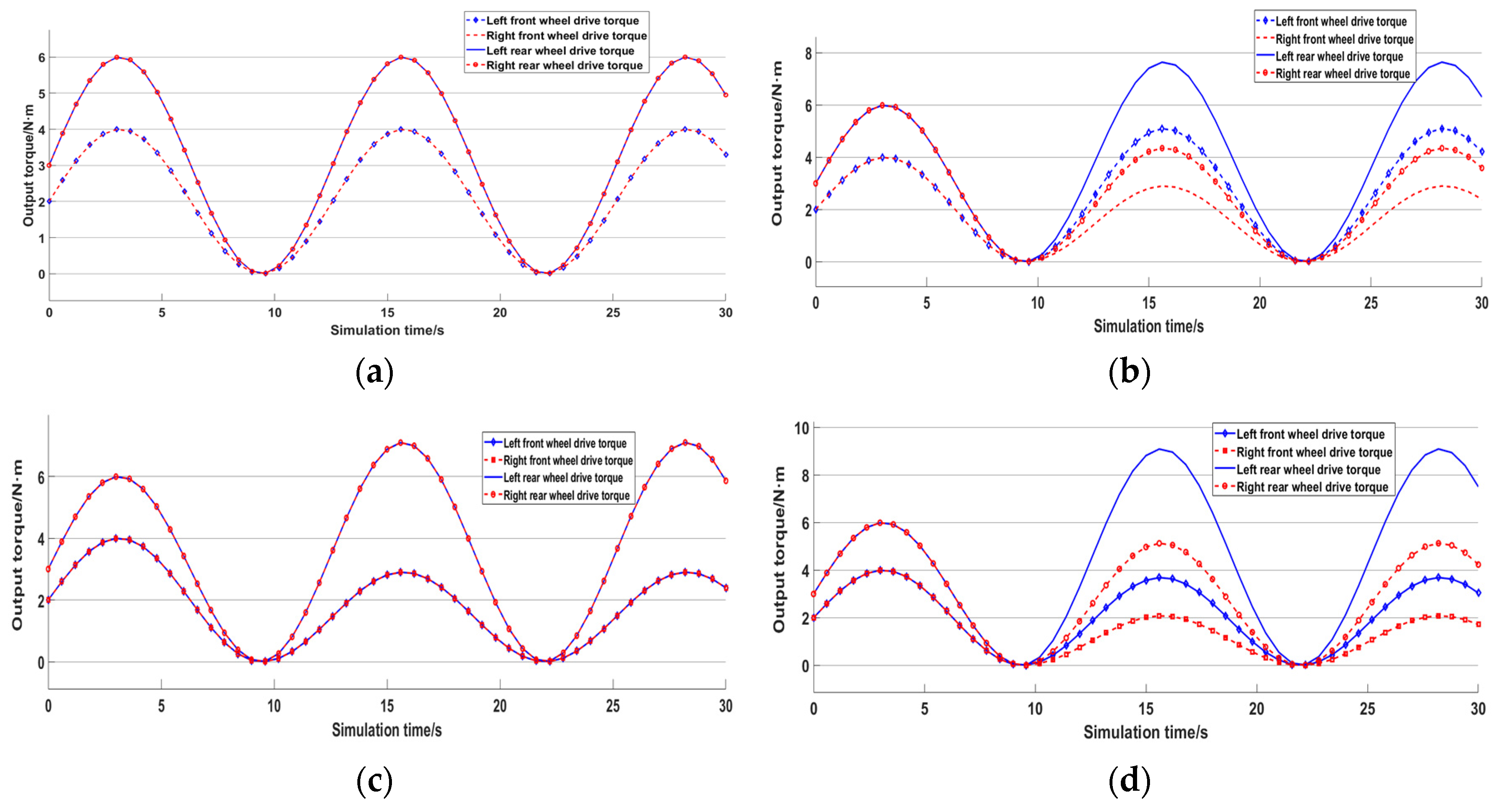
3.1.1. Four-Wheel Torque Distribution Strategy Validation

To validate the constructed four-wheel torque distribution model, simulations were conducted under four different scenarios in the sprayer: when the sprayer’s body pitch angle is 0°, when the sprayer does not have any lateral or pitch angles, when both lateral and pitch angles are 0°, and when they are both non-zero. To ensure that the simulation test aligns with the actual operating conditions, a survey of the actual transportation environment for the sprayer revealed that the majority of road gradients are less than 10°. Consequently, we have set a gradient of 10° as the value for the sprayer’s travel during operation. The simulation scenarios were set as follows:

Scenario 1: The sprayer travels on a level road with no lateral or pitch angles in the body. The input whole-vehicle desired torque is set as a sine wave signal with amplitudes, biases, and frequencies of 100, 100, and 0.5, respectively. The simulation duration is 30 s, and the torque curves of each wheel hub motor output are illustrated in Figure 11a.

Scenario 2: The sprayer travels on a level road from 0 to 10 s and then on a slope from 10 to 30 s with a heading angle of 90°, resulting in a 10° lateral tilt angle of the body and 0° pitch angle. The input signal is the same as in Scenario 1, and the torque curves of each wheel hub motor output are shown in Figure 11b.

Scenario 3: The sprayer travels on a level road from 0 to 10 s and then on a slope from 10 to 30 s with a heading angle of 0°, resulting in a 10° pitch angle of the body and 0° lateral tilt angle. The input signal matches Scenario 1, and the torque curves of each wheel hub motor output are depicted in Figure 11c.

Scenario 4: The sprayer travels on a level road from 0 to 10 s and then on a slope from 10 to 30 s with a 10° pitch angle and a 10° lateral tilt angle of the body. The input signal corresponds to Scenario 1, and the torque curves of each wheel hub motor output are displayed in Figure 11d.

The analysis of the torque distribution simulation results for the four scenarios reveals the following:

(1)

In Scenario 1, as the sprayer operates on a level road, using the sprayer’s center of gravity position as the optimal torque distribution reference, it is determined from the established mathematical model that the center of gravity is located in the rear half of the sprayer, with equal mass on both sides. Consequently, the torque applied to the two rear wheels is equal and slightly greater than that applied to the front wheels.

(2)

In Scenario 2, during the first 10 s, the torque distribution is similar to Scenario 1. After 10 s, when the sprayer ascends the slope, with the left two wheels of the sprayer positioned lower due to the center of gravity being towards the rear, the left rear wheel should have the highest driving torque.

(3)

In Scenario 3, the torque distribution during the first 10 s aligns with Scenario 1. After 10 s, when the sprayer climbs the slope, the torque applied to the two rear wheels is equal, as is the torque applied to the two front wheels, with the rear wheel torque exceeding that of the front wheels.

(4)

In Scenario 4, the torque distribution during the first 10 s is consistent with Scenario 1. After 10 s, when the sprayer ascends the slope with a 10° pitch angle and lateral tilt, the left rear wheel has the highest driving torque.

The simulation results indicate that the torque allocated by the torque distribution module corresponds to the actual force distribution on each wheel, enabling the sprayer to output more reasonable torque when driving on slopes, thereby ensuring stability and safety during operation.

3.1.2. Cruise Control Function Verification

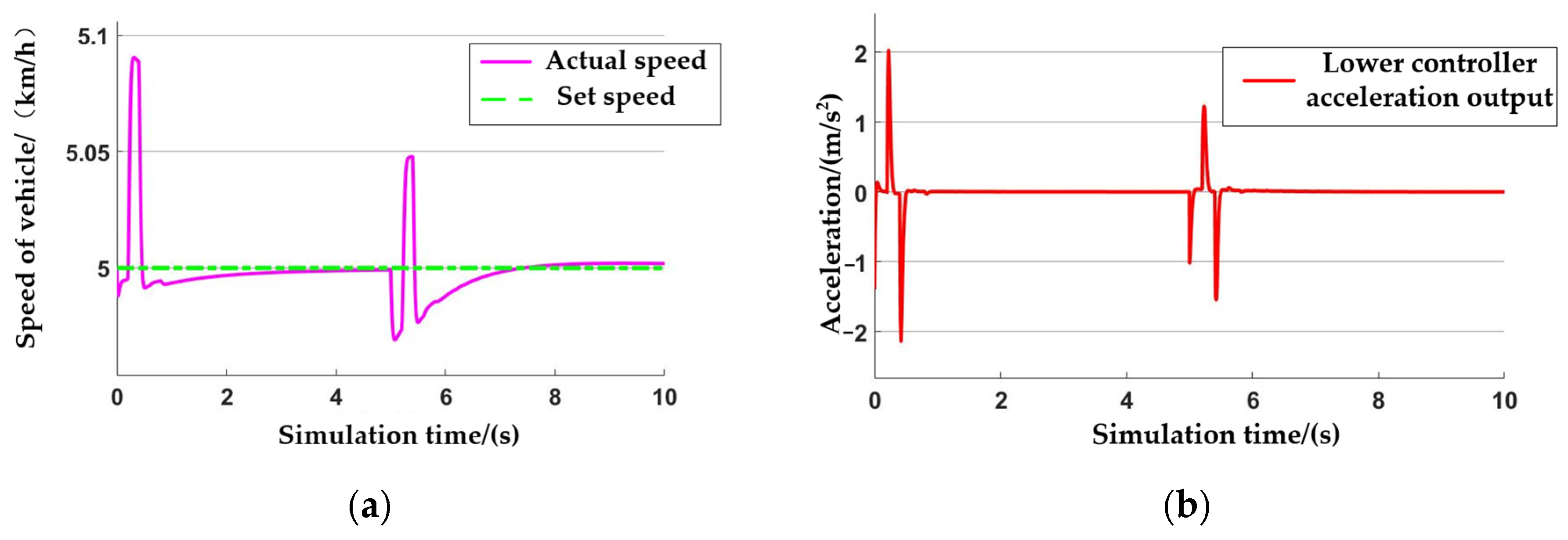
Building upon the established longitudinal dynamics system model and control model, simulations were conducted for the cruise control of the sprayer, considering the actual operational requirements for spray coverage and driving safety. Typically, the sprayer operates at speeds of 3–8 km/h to maintain operational efficiency. Therefore, simulations were conducted under two typical scenarios based on the actual operating speeds of the sprayer:

(1)

The effectiveness of the set speed cruise control during the sprayer’s transition and transport was validated. The following typical scenario was simulated: the sprayer travels on a level road with an initial speed of 5 km/h and zero initial acceleration, maintaining a constant weight. To test the robustness of the control system, an external disturbance in the form of a slope change was introduced between 5 and 10 s, causing the body of the sprayer to pitch at a 10° angle. The simulation results for speed and acceleration are illustrated in Figure 12a,b.

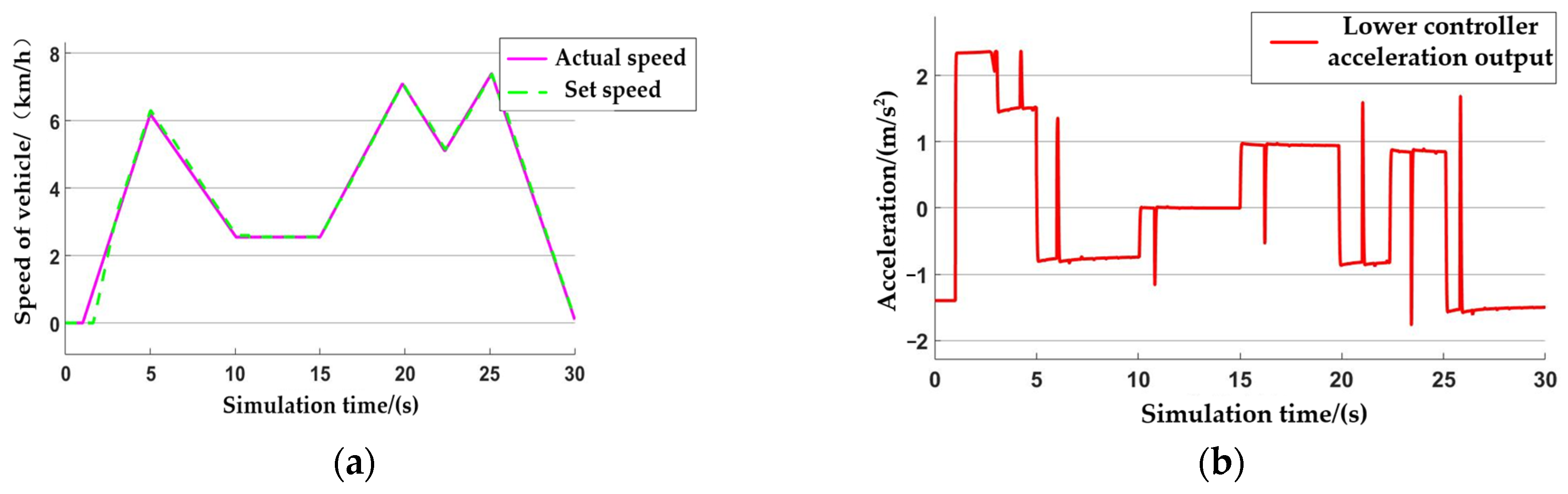
The simulation revealed that the system exhibits a short speed response time of less than 0.1 s, with a maximum steady-state error close to 0 and an overshoot of 1.6%. At 5 s, the system demonstrated sensitivity to slope changes, responding quickly to alterations in the body posture and returning to stability within 2 s.

(2)

The cruise control performance during spraying operations was validated under the following typical scenario: the sprayer starts from rest in the field and periodically adjusts the set desired speed. Additionally, as the spraying operation progresses, the sprayer’s weight gradually decreases. Starting from 15 s until the end of the simulation, a 10° pitch disturbance was introduced. The simulation results for speed and acceleration are shown in Figure 13a,b.

The simulations indicated that even when facing continuous adjustments to the desired vehicle speed by the user, the cruise control system maintained excellent speed tracking performance. The system exhibited a response time of less than 0.2 s, minimal overshoot, and minimal steady-state errors. Furthermore, it demonstrated good robustness in the face of external disturbances such as changes in road slope.

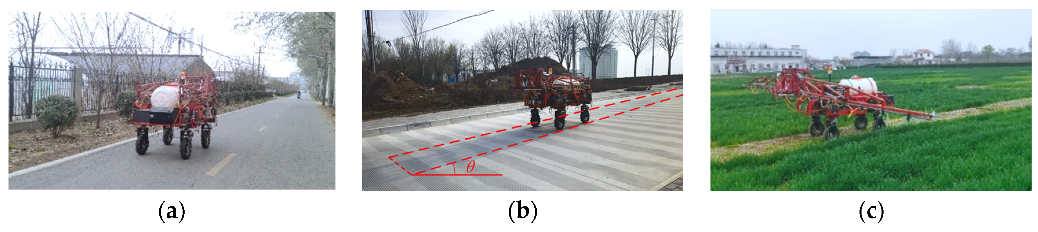
3.2. Analysis of Field Vehicle Test Results

Real vehicle tests were conducted based on the actual working conditions of the self-propelled sprayer, focusing on transition transportation and field operations. To comprehensively evaluate the effectiveness of the sprayer’s cruise control function under different road conditions, the experimental plan included on-road testing on cement, asphalt, and compacted soil surfaces in the field. The cement surface was utilized to assess the machine’s speed maintenance capability when encountering slopes during straight-line horizontal travel, while the asphalt surface was used to evaluate the cruise control function during routine transition transportation. On the compacted soil surface in the field, the cruise control function during actual spraying operations was validated. The experimental conditions and grouping are presented in

Table 3. Test grouping and condition setting.

Test Scene	Test Grouping	Road Conditions	Driving Conditions
Transit transportation	Group 1	Asphalt concrete roads	Accelerate in a straight line to a constant speed
	Group 2	Concrete pavement	Driving straight uphill
Field operations	Group 3	Compacted dirt road	Accelerate in a straight line to a constant speed

, and the experimental process is illustrated in Figure 14.

3.2.1. Transit Transportation Test

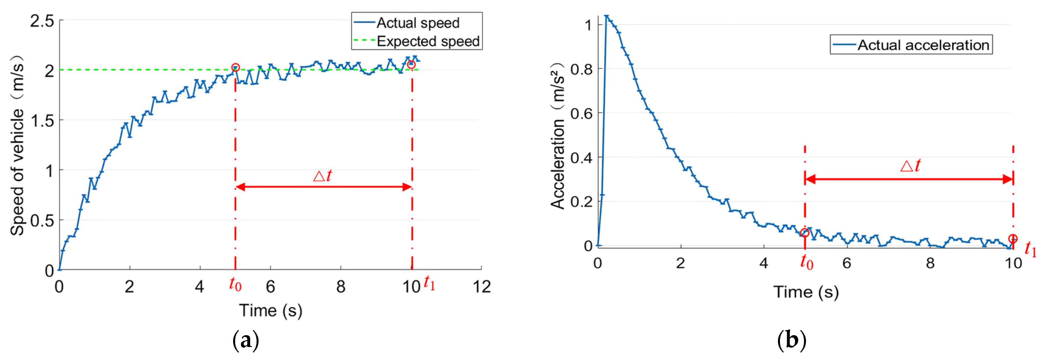
Horizontal Straight-Line Acceleration

During the transition transportation process, the power lever on the remote controller was manipulated to initiate the sprayer’s movement from a standstill. Once the vehicle reached the desired speed, the “Cruise Control” button was pressed. At this point, the control system utilized the current speed signal to regulate the output torque of the wheel motor, ensuring the vehicle maintained the set speed.

The current speed and acceleration of the sprayer were calculated using sensors and transmitted to the upper computer through the controller for storage. During data processing, a low-pass filtering method was employed to eliminate high-frequency interference stemming from the sensors themselves or the environment, while preserving the low-frequency components related to the movement of the sprayer. The specific parameter variations are depicted in Figure 15.

Figure 15a,b depict the speed and speed variation of the sprayer from acceleration to activating the cruise control function. At time t₀ in the figures, the “Cruise Control” function is enabled, with the current set speed being 2 m/s. The total duration of cruise control is symbolized by Δt. To accurately determine the fluctuation and stability between the actual and desired speeds, the start and end times of cruise control are identified as 5 s and 10 s, respectively. By processing the velocity and acceleration data during the Δt period,

Table 4. The results of parameter processing under transfer transportation—linear acceleration.

Parameter Name	Maximum Values	Minimum Value	RMS Value
Speed (m/s)	2.13	1.85	1.91
Acceleration (m/s2)	0.08	−0.01	0.06

is obtained.

Combining Figure 15 and Table 4 reveals that during the transition transportation and straight-line acceleration scenario, the sprayer maintains a stable driving state due to the good road conditions. The acceleration during the cruise control phase remains around 0 m/s², with a root mean square value of 0.06 m/s². As can be observed from Figure 15b, there is a decreasing trend in the acceleration values from time t₀ to t₁. This stable acceleration ensures a small deviation between the speed and the desired value, with a maximum deviation of 0.15 m/s and a maximum deviation rate of 7.5%. The root mean square (RMS) deviation from the expected value is 4.5%, indicating that the velocity of the sprayer gradually stabilizes upon activation of the “constant speed cruise control” feature.

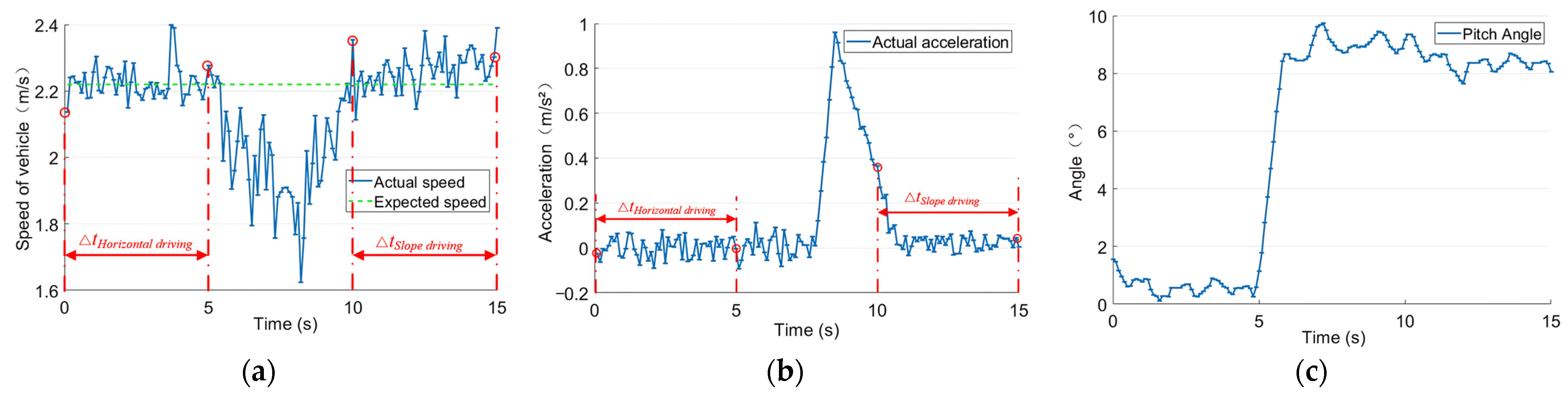
Straight-Line Uphill Driving

To assess the control effectiveness of the cruise control function during uphill travel, the sprayer was maneuvered to a road section with a slope. Prior to ascending the slope, the sprayer was engaged in horizontal straight-line cruise control. The specific parameter variations throughout this entire process are illustrated in Figure 16. By analyzing the velocity, acceleration, and vehicle pitch angle data during this timeframe,

Table 5. The parameter processing results of transfer transportation—straight uphill driving.

Parameter Name	Maximum Values	Minimum Value	RMS Value
Speed when traveling horizontally (m/s)	2.39	2.14	2.24
Speed when traveling uphill (m/s)	2.38	2.11	2.28
Acceleration while traveling horizontally (m/s2)	0.08	−0.09	0.063
Acceleration when traveling uphill (m/s2)	0.27	−0.03	0.221
Pitch angle when traveling horizontally (°)	1.55	0.12	1.47
Pitch angle when traveling uphill (°)	9.35	7.64	8.42

was generated. During the processing of the collected pitch angle data, the utilization of the Kalman filter effectively eliminates noise and drift in the attitude sensor.

In Table 5, “horizontal travel” and “slope travel” refer to stable phases, excluding the transition from horizontal to sloped roads. As shown in Figure 16c, the horizontal travel period for the sprayer spans 0–5 s, while the slope travel period ranges from 10 to 15 s. Upon examination of Figure 16 and Table 5, it is evident that the sprayer was in the constant speed phase for the initial 5 s, during which an expected velocity of 8 km/h (2.22 m/s) was set. Analysis of the data reveals that the root mean square (RMS) value is 2.24 m/s, with a deviation of 0.9% from the expected velocity. Furthermore, the RMS value of acceleration is 0.063 m/s². The sprayer maintained nearly constant speed during this phase, demonstrating effective control under cruise control.

At 5 s, the sprayer transitioned from horizontal to uphill travel. Under the influence of the gravitational component and frictional forces, the sprayer’s velocity decreased rapidly. During the time period of 5–6 s, the sprayer was in a transition phase from horizontal to inclined terrain navigation. Due to the swift change in the pitch angle of the sprayer’s body, the controller did not immediately adjust the speed. After 6 s, the sprayer reached a stable state of traversal on the inclined surface. Approximately 1.5 s later, the controller initiated a response to adjust the vehicle speed, and within 2.5 s, the speed was swiftly restored to the desired value. Concurrently, the pitch angle of the sprayer’s body reflected the slope gradient, with Table 5 indicating a slope of approximately 8.42° during inclined operation. The root mean square (RMS) value of the velocity was 2.28 m/s, with a deviation of 2.7% from the desired value. These data demonstrate that even during inclined traversal, the constant speed cruise control function can essentially maintain the vehicle speed within the desired range. The system’s overall response time was 1.5 s, with an adjustment duration of 2.5 s, indicating a control effect that is relatively accurate.

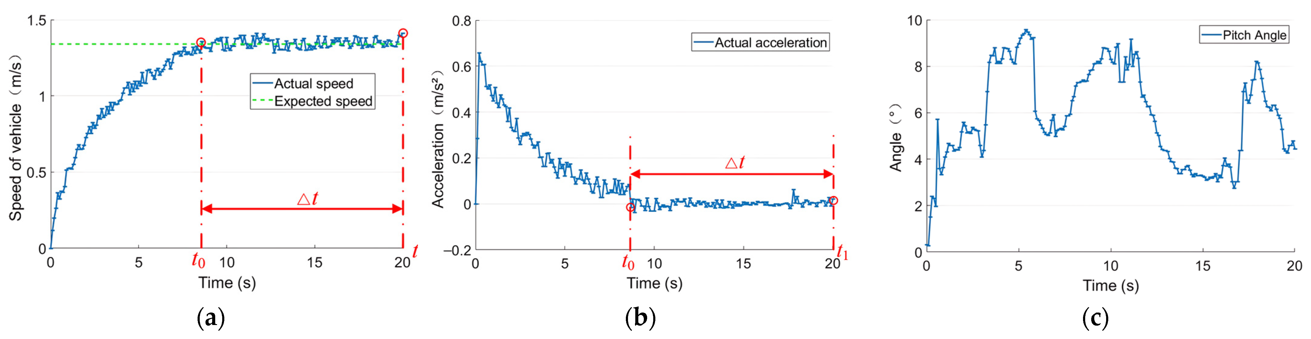
3.2.2. Fieldwork Trials

During field operations, considering the impact of the swaying motion of the spray boom on the quality of pesticide application, both the vehicle speed and acceleration were maintained at low values to mitigate this issue. After driving the sprayer onto the field road and deploying the spray boom, the operator used a remote controller to initiate forward movement for spraying operations starting from a standstill. Upon reaching the desired operational speed, the “Cruise Control” button was pressed, allowing the control system to adjust the wheel motor torque based on the current speed signal to maintain the set speed. Additionally, to visually represent the impact of field roads on the vehicle, the pitch angle of the vehicle was monitored to indicate the roughness of the terrain. Initially, the pitch angle during flat ground travel was measured, and after obtaining and filtering pitch angle data during field travel, the specific parameter variations were presented in Figure 17.

Figure 17a,b illustrate the speed and speed variation of the sprayer from acceleration to activating the cruise control function. At time t₀ in the figures, the “Cruise Control” function was engaged, with the desired speed set at 5 km/h, and the total duration of cruise control is symbolized by Δt. From Figure 17b, it is evident that to ensure stability during spraying, the maximum controlled acceleration is kept below 0.65 m/s². Figure 17c shows significant variations in the pitch angle of the vehicle while traveling on field roads, with a maximum value approaching 10°, indicating random and substantial road disturbances. In the initial acceleration phase, the pitch angle rapidly increases due to the high instantaneous acceleration, reflecting the actual conditions of the sprayer. Summarizing the data collected during the cruise control phase yields

Table 6. Field operation—parameter processing results under linear acceleration.

Parameter Name	Maximum Values	Minimum Value	RMS Value
Speed (m/s)	1.41	1.28	1.35
Acceleration (m/s2)	0.64	−0.03	0.013
Pitch angle (°)	9.24	2.89	13.74

.

Overall, the combination of Figure 17 and Table 6 demonstrates that despite random road disturbances, the sprayer effectively maintains speed. The root mean square velocity is 1.35 m/s, with a deviation rate from the desired speed of 2.8%. The maximum deviation observed was merely 0.1 m/s, with the highest deviation rate being 7.2%. This indicates that the sprayer maintains good cruise control even during field spraying operations. The lower speed and the decrease in the center of gravity due to the lowering of the spray boom during spraying contribute to the enhanced stability of the vehicle under similar conditions.

4. Discussion

Due to changes in road gradient and variations in equipment weight during spraying, the stability of the sprayer is compromised. This study focuses on addressing the speed stability issues encountered by the 4WID high ground clearance self-propelled electric sprayer during driving and spraying operations. The approach involves the analysis of the sprayer’s structure and longitudinal dynamic characteristics, utilizing a hierarchical control structure that combines upper-layer PID and lower-layer fuzzy PID algorithms to manage the entire system. The research encompasses the development of a dynamic model considering driving resistance, slope, and vehicle roll angle effects on the distribution of the four-wheel load, along with field tests to validate the model and control theory.

Key findings of this study include the following:

(1)

Establishment of a dynamic model for slope driving conditions based on an analysis of the sprayer’s longitudinal dynamic characteristics.

(2)

Implementation of simulation experiments under external disturbances and variations in vehicle weight using a hierarchical control structure with upper-layer PID and lower-layer fuzzy PID control. Results indicate rapid speed adjustment response times of less than 0.1 s, with an overshoot of only 1.6%. The control system demonstrates effective speed tracking capabilities across various simulated scenarios.

(3)

Evaluation of the stability of the sprayer’s cruise control function through on-road tests using a sensor-equipped test platform. Results show minimal speed deviation and effective maintenance of stable speed during straight-line acceleration and uphill driving scenarios.

During the research process, it was assumed that the sprayer wheels do not slip, and the speed of each wheel can be calculated from the vehicle speed. The internal speed of the hub motor can be determined from the reduction ratio of the hub motor. Consequently, in real vehicle experiments, when the vehicle speed needs to be altered, the controller adjusts the magnitude of the analog voltage signal input to the hub motor driver. The driver then increases or decreases the current input to the hub motor, ultimately controlling the motor speed to achieve the desired speed.

Additionally, due to the nonlinear nature of the overall dynamic system, a hierarchical control approach was adopted in the controller design process, utilizing linear PID and nonlinear fuzzy PID. The design of the fuzzy PID controller addressed the limitations of traditional PID controllers in nonlinear systems. By incorporating fuzzy logic, the fuzzy PID controller can flexibly adjust its control strategy when facing nonlinear responses, thus better adapting to changes in system dynamic behavior. The combination of these two controllers resolved stability issues that might arise from directly applying traditional PID control in nonlinear systems, enhancing the overall adaptability and robustness of the control system.

Based on the above analysis, to make the model more realistic and improve control stability, future research will focus on the following aspects:

(1)

Considering the slip of each wheel during sprayer operation, incorporating slip rate control to enhance the precision of torque control.

(2)

Building upon the existing research, introducing advanced control techniques such as adaptive control, sliding mode control, or other more complex nonlinear control methods to more accurately capture the system’s nonlinear characteristics, thereby designing more efficient and reliable control strategies.

5. Conclusions

(1)

Based on the analysis of the longitudinal dynamic characteristics of a self-propelled electric sprayer on sloped terrain, a simplified model of the sprayer’s dynamic system was established by combining relevant vehicle data under the assumption of simplification.

(2)

Simulation experiments were conducted using a hierarchical control structure based on upper-level PID control and lower-level fuzzy PID control, considering external disturbances and variations in vehicle weight. The results showed that the system had a very short response time for speed adjustment, less than 0.1 s, with an overshoot of only 1.6%. In the simulation experiments involving simultaneous variations in vehicle weight and slope, the control system exhibited a response time of less than 0.2 s, with minimal overshoot and steady-state errors. These three sets of simulation experiments verified the rationality of the torque distribution algorithm and the effectiveness of the cruise control algorithm in tracking the vehicle speed.

(3)

An experimental platform for the entire vehicle chassis was built on the actual vehicle to evaluate the stability of the cruise control function of the sprayer by collecting acceleration and velocity data using sensors. During the horizontal straight-line acceleration phase in transportation transition, the measured maximum deviation in speed was 0.15 m/s, with a maximum deviation rate of 7.5%. The acceleration remained close to zero during the cruise control phase, with a root mean square value of 0.06. During the straight-line uphill travel phase in transportation transition, the root mean square velocity values during stable travel (horizontal and uphill phases) were 2.24 m/s and 2.28 m/s, respectively, with deviation rates from the desired values of 0.9% and 2.7%. During field operations, the root mean square velocity of the sprayer was 1.35 m/s, with a deviation rate from the desired speed of 2.8%. The experimental results further validated the correctness of the model construction and the rationality and accuracy of the experiments, providing strong support for the cruise control of the sprayer.

References

1. Tang, H.; Han, J.; Yan, X. Path Navigation Control Method of Tractor Rotary Cultivator Group Based on Lateral Force Limitation. J. Agric. Mech. Res. 2024, 46, 32–37. [Google Scholar]
2. Wu, C.; Wu, S.; Wen, L.; Chen, Z.; Yang, W. Variable curvature path tracking control for the automatic navigation of tractors. Trans. Chin. Soc. Agric. 2022, 38, 1–7. [Google Scholar]
3. Wang, S.; Li, Q.; Zhu, H. Design of simulation test platform for autonomous navigation of orchard vehicles. J. Chin. Agric. Mech. 2024, 45, 132–140. [Google Scholar]
4. Wan, X.; Wang, H.; Cong, P.; Xiao, Y.; Zhao, R.; Chen, X.; Liu, J. Study on localization algorithm of monocular vision navigation for orchard spraying robot. J. Agric. Sci. 2023, 51, 202–209. [Google Scholar]
5. Jiang, C.; Zhang, L.; Gu, H. Design and Test of Positioning System of Agricultural Harvester Based on Information Age. J.Agric. Mech. Res. 2021, 43, 195–198. [Google Scholar]
6. Li, Z.; Liu, X.; Chen, X.; Gao, Y.; Yang, S. Tractor Integrated Navigation and Positioning System Based on Data Fusion. Trans. Chin. Soc. Agric. 2020, 51, 382–390+399. [Google Scholar]
7. Han, K.; Zhu, Z.; Mao, E.; Song, Z.; Xie, B.; Li, M. Joint Control Method of Speed and Heading of Navigation Tractor Based on Optimal Control. Trans. Chin. Soc. Agric. 2013, 44, 165–170. [Google Scholar]
8. Wang, Z.; Liu, Z.; Bai, X.; Gao, L. Longitudinal Acceleration Tracking Control of Tractor Cruise System. Trans. Chin. Soc. Agric. 2018, 49, 21–28. [Google Scholar]
9. Zhao, C.; Wei, C.; Fu, W.; Shang, Y.; Zhang, G.; Cong, Y. Design and Experiment of Cruise Control System for Hydrostatic Transmission Tractor. Trans. Chin. Soc. Agric. 2021, 52, 359–365. [Google Scholar]
10. Xie, L.; Luo, Y.; Li, S.; Li, K. Coordinated Control for Adaptive Cruise Control System of Distributed Drive Electric Vehicles. Automot. Eng. 2018, 40, 652–658+665. [Google Scholar]
11. Zhang, G.; Wang, Y.; Wang, F.; Meng, Y. Research on Stability of Adaptive Cruise Based on DDEV. Mach. Build. Autom. 2023, 52, 190–193+221. [Google Scholar]
12. Zhang, L.; Liu, M.; Liu, Z.; Xie, L. Joint Simulation of Vehicle Adaptive Cruise Hierarchical Control System. Mach. Des. Manuf. 2022, 69–72+77. [Google Scholar] [CrossRef]
13. Dong, S.; Yuan, Z.; Gu, C.; Yang, F. Research on intelligent agricultural machinery control platform based on multi-discipline technology integration. Trans. Chin. Soc. Agric. 2017, 33, 1–11. [Google Scholar]
14. Han, S.; He, Y.; Fang, H. Recent development in automatic guidance and autonomous vehicle for agriculture: A Review. J. Zhejiang Univ. (Agric. Life Sci.) 2018, 44, 381–391+515. [Google Scholar]
15. Coen, T.; Saeys, W.; Missotten, B.; De, B.J. Cruise control on a combine harvester using model-based predictive control. Biosyst. Eng. 2008, 99, 47–55. [Google Scholar] [CrossRef]
16. Kayacan, E.; Ramon, H.; Ramon, H. Towards agrobots: Trajectory control of an autonomous tractor using type-2 fuzzylogic controllers. IEEE-ASME T Mech. 2015, 20, 287–298. [Google Scholar] [CrossRef]
17. Miao, Z.; Li, C.; Han, K.; Hao, F.; Han, Z.; Zeng, L. Optimal Control Algorithm and Experiment of Working Speed of Cotton-picking Machine Based on Fuzzy PID. Trans. Chin. Soc. Agric. 2015, 46, 9–14+27. [Google Scholar]
18. He, J.; Zhu, J.; Zhang, Z.; Luo, X.; Gang, Y.; Hu, L. Design and Experiment of Automatic Operation System for Rice Transplanter. Trans. Chin. Soc. Agric. 2019, 50, 17–24. [Google Scholar]
19. Shen, Y.; He, S.; Liu, H.; Cui, Y. Modeling and control of self-steering electric chassis structure of high clearance sprayer. Trans. Chin. Soc. Agric. Mach. 2020, 51, 385–392, 402. [Google Scholar]
20. Wang, Z.; Lv, G.; Zhu, X. Research on the measurement method of vehicle driving resistance. Automob. Appl. Technol. 2019, 67–69. [Google Scholar]
21. Song, Q.; Wang, G.; Shang, H.; Zhang, N. Research on Handling Stability Control Strategy for Distributed Drive Electric Vehicle Based on Multi-parameter Control. Automot. Eng. 2023, 45, 2104–2112+2138. [Google Scholar]
22. Li, Z.; Pan, S.; Xu, Y. Review on Cooperative Control of Chassis Stability for Distributed Electric Vehicles. Automob. Technol. 2022, 9, 1–14. [Google Scholar]
23. Qi, L.; Lv, X.; Wang, L. Analysis and simulationon force distribution ratio of AWD vehicle. Mach. Des. Manuf. 2011, 181–183. [Google Scholar]
24. Sangeetha, E.; Subashini, N.; Santhosh, T. Validation of EKF based SoC estimation using vehicle dynamic modelling for range prediction. Electr. Power Syst. Res. 2024, 226, 109905. [Google Scholar]
25. Sun, B.; Gu, T.; Wang, P.; Zhang, T.; Shubin, W. Optimization Design of Powertrain Parameters for Electromechanical Flywheel Hybrid Electric Vehicle. IAENG Int. J. Appl. Math. 2022, 14, 11017. [Google Scholar]
26. Li, R.; Deng, S.; Hu, Y. Autonomous Vehicle Modeling and Velocity Control Based on Decomposed Fuzzy PID. Int. J. Fuzzy Syst. 2022, 24, 2354–2362. [Google Scholar] [CrossRef]
27. Sun, W.; Rong, J.; Wang, J.; Zhang, W.; Zhou, Z. Research on Optimal Torque Control of Turning Energy Consumption for EVs with Motorized Wheels. Energies 2021, 14, 6947. [Google Scholar] [CrossRef]
28. Hu, F.; Chen, L.; Hu, D.; Chen, W. 4WD Car Performance Study Based on Electronic Stability and Torque Distribution Coordinated Control. J. Mech. Eng. 2017, 53, 147–157. [Google Scholar] [CrossRef]
29. Schreiber, M.; Kutzbach, H.D. Influence of soil and tire parameters on traction. Res. Agric. Eng. 2008, 54, 43–49. [Google Scholar] [CrossRef]
30. Roth, J.; Darr, M. Data acquisition system for soil-tire interface stress measurement. Comput. Electron. Agric. 2011, 78, 162–166. [Google Scholar] [CrossRef]
31. Fan, B.; Hui, K.; Zhang, B.; Lu, D. Analysis of Tire Cornering Stiffness Property under Slight Driving or Braking Condition. J. Appl. Biomater. Biom. 2012, 271–272, 767–772. [Google Scholar]
32. Zhang, K.; Zhang, Y.; Xu, P. An Algorithm for Parameter Identification of Semi-Empirical Tire Model. SAE Int. J. Veh. Dyn. Stab. NVH 2021, 5, 379–396. [Google Scholar] [CrossRef]
33. Du, H.; Gao, Z.; Liu, Z. Research status and development trend of automobile tire model. Tire Ind. 2019, 39, 195–198. [Google Scholar]
34. Yuan, Z.; Lu, D.; Guo, K. Comparative Study on the UniTire Model and the Magic Formula Model. Automob. Technol. 2006, 7–11. [Google Scholar]
35. Guo, K.; Lu, D. UniTire: Unified tire model for vehicle dynamic simulation. Veh. Syst. Dyn. 2007, 45 (Suppl. S1), 79–99. [Google Scholar] [CrossRef]
36. Duan, S.; Xu, N.; Shi, Q.; Bai, X. Longitudinal Dynamic Model of Tire Considering Hysteresis Characteristics. J. Mech. Eng. 2023, 59, 364–372. [Google Scholar]
37. Chen, W.; Wang, S. Four-Wheel AGV Transporter Straight-Line Movement PID Control and Implementation. Autom. Appl. 2024, 65, 94–96+105. [Google Scholar]
38. Huang, J.; Wang, X.; Gao, Y.; Liu, H. Research on path planning and tracking control of four-wheeled independently driven electric vehicles. Mech. Sci. Technol. Aerosp. Eng. 2024, in press.
Figure 1. Equipment for real vehicle test: (a) attitude sensor; (b) IMC T3654 controller; (c) remote controller.
Agriculture 14 00902 g001
Figure 2. High-clearance, self-propelled sprayer test platform.
Agriculture 14 00902 g002
Figure 3. Force diagram of the sprayer in a spatial coordinate system. M—total weight of sprayer, kg; L—sprayer wheelbase, m; la—center of mass to front axle distance, m; lb—center of mass to rear axis distance, m; B—wheel pitch, m; h—height of center of mass, m; V—current traveling speed, m/s2; Fw—air resistance, N; Fa—acceleration resistance, N; Fp–ramp resistance, N; Ttqij—optimum demand torque for each wheel, N·m; Ftij—driving force of each wheel individually, N; FNij—normal ground support for each wheel, N; Ffij—rolling resistance of each wheel, N; (i = f,r; j = l,r).
Agriculture 14 00902 g003
Figure 4. Longitudinal dynamics simulation system of the sprayer. ades—desired model acceleration; Tdes—desired total driving or braking torque; T1des, T2des, T3des, T4des—desired torques for each wheel; T1, T2, T3, T4—actual output torques for each wheel; vf—actual speed; af—actual acceleration.
Agriculture 14 00902 g004
Figure 5. Schematic representation of the forces on the sprayer from two viewpoints: (a) two-wheel model of the sprayer from a pitch angle view; (b) two-wheel model of the sprayer from a pitch angle view.
Agriculture 14 00902 g005
Figure 6. Motor model construction: (a) motor external characteristics curve; (b) motor modeling in Simulink.
Agriculture 14 00902 g006
Figure 7. Sprayer chassis dynamics modeling: (a) schematic diagram of vehicle 7-DOF model; (b) wheel dynamics model. vwx_ij—longitudinal speed of wheel center; ωwij—angular velocity of wheel rotation; Ffij—longitudinal force on wheels; FNij—ground support.
Agriculture 14 00902 g007
Figure 8. Overall scheme of the cruise control system for the sprayer.
Agriculture 14 00902 g008
Figure 9. Corresponding characteristic curves of input and output variables: (a) the input variable corresponds to the characteristic surface of Kp; (b) the input variable corresponds to the characteristic surface of Ki; (c) the input variable corresponds to the characteristic surface of Kd..
Agriculture 14 00902 g009
Figure 10. Overall model of cruise control at constant speed.
Agriculture 14 00902 g010
Figure 11. Torque distribution of individual wheel hub motors under different operating conditions: (a) working condition 1; (b) working condition 2; (c) working condition 3; (d) working condition 4.
Agriculture 14 00902 g011
Figure 12. Parameters of cruise control simulation under working conditions: (a) speed tracking curve; (b) acceleration output curve.
Agriculture 14 00902 g012
Figure 13. Parameters of cruise control simulation under working condition II: (a) speed tracking curve; (b) acceleration output curve.
Agriculture 14 00902 g013
Figure 14. Vehicle test process: (a) Group 1; (b) Group 2; (c) Group 3.
Agriculture 14 00902 g014
Figure 15. The actual parameters of the sprayer under the transfer transportation—linear acceleration: (a) velocity variation; (b) acceleration change.
Agriculture 14 00902 g015
Figure 16. Transfer field transportation—actual parameters of straight uphill driving sprayer: (a) velocity variation; (b) acceleration change; (c) body pitch angle changes.
Agriculture 14 00902 g016
Figure 17. Field operation—actual parameters of sprayer under linear acceleration: (a) velocity variation; (b) acceleration change; (c) body pitch angle changes.
Agriculture 14 00902 g017