Abstract
At present, agricultural non-point source pollution has become the main source of water pollution, which mainly comes from the excessive use of agricultural chemicals such as pesticides and fertilizers. The TRS is another land system reform in China after the household contract responsibility system, which relaxes the management rights of rural land and clarifies the ownership of land. Using this land reform in China as a case study, this paper constructs panel data for 30 provinces in China to explore the impact of land tenure intensification on agricultural non-point source pollution, using the difference-in-difference (DID) model to identify the causal relationship between the two. The results show that the coefficient of the TRS policy variable is −4.056 at the 1% significance level, indicating that this round of land reform has suppressed agricultural non-point source pollution. The provinces that have implemented TRS have seen an average annual reduction of 405,600 tons in Agnps emissions compared to those that have not implemented TRS, and the scale operation of agriculture and the size of the agricultural economy act as two paths. Moreover, heterogeneity analysis shows that the policy effect of the provinces in non-major food-producing areas is smaller than that of the provinces in major food-producing areas, and the path to realization is also different. Therefore, we should continue to encourage large-scale agricultural operations, cultivate new agricultural business entities, and strengthen the inhibitory effect of TRS on agricultural non-point source pollution.
1. Introduction and Literature Review
Agricultural non-point source pollution (hereinafter abbreviated as Agnps), which refers to the contamination of water bodies by pollutants generated during the agricultural production process through pathways such as surface runoff and subsurface leaching, has become a major source of surface water and groundwater pollution worldwide, with 30% to 50% of the Earth’s surface already affected by non-point source pollution [1]. According to the Food and Agriculture Organization of the United Nations’ “2020 Yearbook of World Food and Agriculture Statistics”, there was a significant increase in global pesticide usage from 2000 to 2018, reaching 4.1 million tons annually, which is a one-third increase. Concurrently, the use of chemical fertilizers has also risen, with the total amount increasing to 53 million tons, equivalent to approximately 121 kg per hectare of farmland. In modern agricultural production, the extensive use of chemical fertilizers, pesticides, and mulch, coupled with inadequate waste management in planting and breeding processes, has led to a substantial influx of nutrients such as nitrogen, phosphorus, and organic matter into the ecosystem, exacerbating the issue of Agnps. These pollutants, through surface runoff and subsurface leaching, have caused severe water pollution, posing threats to water resource safety and ecological balance [2]. Compared to fixed-point source pollution, this type of pollution is typically more widespread and diverse, lacks a clear discharge point, has undefined geographical boundaries, and is characterized by high dispersion, strong concealment, and significant challenges in management and mitigation.
China has been an agricultural powerhouse since ancient times and remains the largest developing country in the world today. Compared to the high labor input and low capital input in agricultural production at the beginning of the nation’s founding, the enhancement of rural wealth brought about by reform and opening up has led to heavy reliance on capital goods such as pesticides and chemical fertilizers, which have become significant reasons for China’s high agricultural output and have long formed a path dependency [3]. Due to this path dependency and consumer orientation, the overuse of chemicals such as pesticides, fertilizers, and agricultural films in large-scale planting has caused severe Agnps in China, becoming one of the major sources of water, soil, and air pollution [4]. According to the data from the “Second National Pollution Source Census Bulletin” released by the Ministry of Ecology and Environment of the People’s Republic of China, in 2017, China’s agricultural source water pollution emissions were 10.6713 million tons of chemical oxygen demand, accounting for 49.7% of the national total water pollution emissions; 216,200 tons of ammonia nitrogen, accounting for 22.4% of the total emissions; 1.4149 million tons of total nitrogen, accounting for 46.5% of the total; and 212,000 tons of total phosphorus, accounting for 67.2% of the total. In the face of the severe agricultural pollution situation, the “Implementation Plan for the Management and Supervision of Agricultural Non-Point Source Pollution (Trial)” was issued in 2021, elevating the governance of agricultural ecology and environment to a national strategy and establishing a policy system for the prevention and control of Agnps. The main reason for China’s current Agnps is the excessive use of agricultural chemicals [5]. Unlike intensive and large-scale agricultural production in countries such as the United States, Germany, and the Netherlands, China still has a prevalence of smallholder economies. Small-scale family operations find it difficult to ensure the application of advanced agricultural technology and machinery, instead adhering to traditional practices and relying on continuous inputs of pesticides and fertilizers to ensure yields. The reasons for this situation are twofold: firstly, most farmers engaged in agriculture in China have a lower level of education and find it difficult to learn and apply new agricultural technologies, thereby changing traditional production concepts [6]; secondly, the land system restricts large-scale production, and smallholder agricultural production always favors the use of pesticides and fertilizers. China’s modern land system has evolved from collective to private ownership, and since the reform and opening up, the household responsibility system with linked production has been implemented. Land contracting rights have been liberalized, and agricultural intensification has gradually begun, but so far, large-scale agricultural production has not taken shape [7,8].
In the historical development of China, the alternation of dynasties has always been accompanied by reforms in the land system, and each dynasty has had different land policies [9]. During the feudal dynasty period, land ownership belonged to the state, while land use rights were given to the farmers. However, after the establishment of the People’s Republic of China, the continuous adjustment and practice of land policies have led to the current system, in which “land use rights belong to the state and collectives, and farmers have the management rights and contracting rights to the land”. From the “two rights separation” of ownership and contracting management rights implemented after the reform and opening up, to the current process of clarifying the management rights and contracting rights, this gradual process of strengthening land tenure is the case study of this paper, “three rights separation” (hereinafter referred to as TRS), which the Chinese government first proposed in 2014. After five years of practice in various provinces, the legal status and rights of land management were officially granted in 2019. Research on the TRS mainly focuses on the economic effects of this policy, which can be divided into micro and macro aspects. Microscopically, the separation of land management rights and contracting rights has a positive effect on increasing farmers’ income [10]. On one hand, the TRS increases the ways for farmers to earn income, allowing them to gain income from both land management and off-farm employment [11]; on the other hand, the TRS increases the collective economic income in rural areas by concentrating land rights on operating entities, achieving economies of scale in agricultural management [12]. Although many studies believe that this reform can promote farmers’ income growth by increasing land transfer, there may be controversy over whether the TRS can accelerate land transfer. Yan and Yang (2021) established an irrational analysis framework, arguing that the separation of land contracting management rights would strengthen the endowment effect of land, causing farmers to overestimate the value of their land and hinder the operation of the land transfer market [13]. Macroscopically, according to the existing literature, the impact of this round of land reform on agriculture and rural areas is diverse. For example, it has improved the efficiency of farmers’ agricultural production management [14], increased total factor productivity by reducing the misallocation of land resources [15], and some scholars have studied the relationship between the three rights transfer and the sustainable development of the agricultural environment, finding that increasing the use of organic fertilizers has reduced agricultural pollution to the environment [16].
In previous studies on the TRS, the focus has often been on the economic benefits brought about by this land reform, and there is already an abundance of related research. However, studies that focus on the environmental benefits are still relatively scarce. To fill this gap in the literature, this paper considers the TRS as a land reform that has intensified land tenure and uses it as a case study to examine the impacts and mechanisms of land system reforms on Agnps. Specifically, this paper employs a difference-in-differences model to examine the policy effect of this land reform and analyzes its internal relationship with the scale of agricultural operations and the economic scale of agriculture. This study finds that TRS can significantly suppress the emission of Agnps, and this effect remains robust under a series of robustness tests. Moreover, the effect and mechanism vary across different provinces. The potential marginal contributions of this paper are as follows: First, based on the existing literature, this paper conducts research on Agnps from the perspective of land ownership changes under land reform, which allows for a more macro-level discussion on the causes and management strategies of Agnps. Second, by using the timing of each province’s response to the TRS policy documents to set policy dummy variables, this paper can estimate a more accurate policy effect. Third, this paper explores the role of land ownership clarification and the relaxation of land management rights in the framework of TRS affecting Agnps, deepening the existing literature.
2. Policy Background and Research Hypothesis
2.1. TRS Policy Background and Its Implications
In 1978, China began implementing the household responsibility system with linked production contracts, which established the separation of land ownership and contract management rights, known as the “two rights separation”. This reform transformed the land system from communal to individual ownership, greatly motivating farmers in their production [17]. As China quickly urbanizes, more farmers are moving to cities and finding jobs outside of farming. This shift has increased the need for land to be transferred. While the right to operate land is not legally recognized, in reality, it is distinct from the right to contract [18]. By 2014, a new round of land reform began, and the TRS was officially implemented. Its key goal was to split land contract management rights into two: contracting rights and operational rights. This change aimed to guarantee a smooth transfer of land management rights [19]. According to property rights theory in new institutional economics, clearly defined property rights encourage individuals to work harder and prevent them from taking advantage of situations, thereby providing momentum for economic development. At the same time, clearly defined and freely transferable private property rights are prerequisites for market formation, and markets are the institutional foundations for the effective allocation of resources. The direct impact of this land reform can be divided into two aspects: the relaxation of land management rights and clearer rights attribution [20]. On one hand, the TRS accelerated land transfer by relaxing land management rights [21,22], and some studies believe that clearer land ownership strengthens the private attributes of land in farmers, which enhances their estimation of land value, thereby increasing the price of farmers’ land in the rental market and increasing operational income [23]. On the other hand, this round of land reform also affects farmers’ behavior, increasing their confidence in long-term land investment [24]. Furthermore, the acceleration of land transfer under the TRS leads to the aggregation of land, forming new types of agricultural operators with scaled production capabilities, such as family farms, agricultural companies, and agricultural cooperatives [25,26]. Scaled agricultural operations, unlike small-scale farming in a smallholder economy, can better withstand risks, and more standardized and planned production processes can reduce production costs. This, in turn, encourages the use of agricultural machinery and modern farming technology [27,28]. When farmers feel secure about their long-term land investment, they will invest in better tools and more efficient farming methods, even if their farm is small, which will also improve agricultural production efficiency [29]. The following are some studies on how agricultural scale and agricultural production efficiency promote agricultural economic growth. Zaid Ashiq Khan (2022) studied the relationship between fertilizer use, carbon emissions, and agricultural economic growth in China, believing that changes in agricultural output value can reflect the growth of the agricultural economy [30]. Duan (2024) argues that as agriculture scales up, the resulting industrialization will drive economic growth in the agricultural sector [31]. Wu (2024) examined the link between agriculturally socialized services and grain production using panel data from Chinese provinces. It was found that these services primarily boost grain output and agricultural economic growth by facilitating the management of large-scale land consolidation [32]. In addition, some studies believe that when farmers’ income structures become more diverse, it will enhance their entrepreneurial awareness, indirectly strengthening the agricultural economy [33]. These studies, which look at agricultural growth from different angles, all point to the same conclusion: as agricultural scale, income, and farmers’ investment in production increase, so does the agricultural economy.
2.2. Research Hypothesis
The previous discussion, building on current research, shows that the TRS reform has a beneficial impact on advancing large-scale farming and boosting the agricultural economy. The following text will discuss how the TRS affects Agnps. This paper posits that there are two main pathways (for a summary of the specific path mechanisms, see Figure 1): First, under the TRS, large-scale agricultural production will invest more in agricultural technology as a substitute for traditional agricultural input factors. Provinces that have adopted the TRS reform offer more subsidies and support for land transfer than those that have not. This encourages the growth of a market for agricultural services, helping them move towards large-scale farming faster than other provinces. For example, after Shandong Province first proposed the TRS pilot project for the entire province in 2015, it emphasized in 2016 the development of a transformation towards agriculturally socialized services, which in turn supports the scaling of agriculture. Local documents on agriculture and rural areas from 2017 and 2018 also frequently highlighted the TRS reform. Moreover, the larger the scale of agriculture, the smaller the marginal cost of investing in a particular technology, and the greater the scale benefits generated by technological investment [34]. Additionally, large-scale production generates more uniform types of pollutants, making it easier to treat pollution, which in turn affects Agnps. For instance, Liu’s research found a positive correlation between the scale of breeding and the rate of pollution treatment [35]. Currently, the overall level of agricultural scale in China is not high, and there is still a significant gap compared to the developed countries. Therefore, the scale of benefits brought about by accelerated land transfer is aiding the development of Chinese agriculture. Based on path one, this paper proposes its first hypothesis: implementing the TRS policy can lead to an expansion of agricultural operations’ scale in the pilot provinces, thereby curbing Agnps, and it is more obvious in provinces with a higher degree of land transfer.
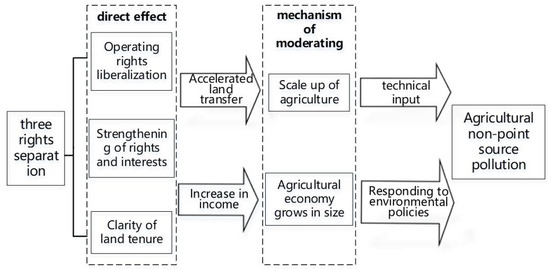
Figure 1.
The Impact of TRS on Agnps.
Secondly, the TRS has strengthened the capacity of regions to respond to environmental protection policies. With the gradual acceleration of land transfer speed and scale, more new types of agricultural operators, such as agricultural cooperatives and companies, have been formed [26]. As the agricultural sector expands, management skills are strengthened and modernized, which better equips the region to meet national and provincial environmental standards for farming. Liu researched how agricultural firms perceive and react to environmental regulations, focusing on their total factor productivity. The analysis revealed that, due to varying resource availability and market conditions, different regions have different capacities to comply with policies [36]. Huang’s research found that the same environmental policy exhibits strong heterogeneity in China’s eastern, central, and western regions. While it can promote green environmental development in the east, the results in the west are quite different [37]. China’s agricultural environmental protection policies emphasize both pollution control and pollution reduction. Therefore, the stronger the region’s capacity to respond to policies, the stronger its ability to manage agricultural pollution. Based on the above, this paper proposes its second hypothesis: the TRS reform has led to an expansion of the agricultural sector in the pilot provinces, enhancing agricultural management capabilities. This has allowed for quicker implementation of environmental protection policies by higher-level authorities compared to non-pilot regions, resulting in a reduction in Agnps emissions.
3. Methods, Variables, and Data
3.1. Model Construction
The TRS policy was officially introduced by the central government in 2014 and subsequently codified into law in 2019. To pinpoint the implementation timeline across various provinces, this study leverages the Peking University Law Database (PKULAW) database to access policy documents and regulations pertaining to the TRS. The year when the first responsive document was issued is taken as the effective date of the policy for each province. The analysis reveals that since the introduction of the TRS in 2014, 19 provinces have issued relevant documents. This paper treats the staggered responses to the TRS as a quasi-natural experiment and employs a difference-in-differences model to assess the impact of the land system reform on Agnps. The model is set up as follows:
In Equation (1), is the explained variable of this paper, representing the Agnps of each province in different years; is the dummy variable of the TRS, indicating whether a certain province implements the policy; is the control variable related to Agnps; in addition, year fixed effect and province fixed effect are added to the model; and is the residual.
3.2. Variable Settings
3.2.1. Explained Variable
Agricultural non-point source pollution (). In this study, key indicators of Agnps are measured using chemical oxygen demand (COD), ammonia nitrogen (NH3-N), total nitrogen (TN), and total phosphorus (TP). Pollutants mainly come from nitrogen and phosphorus in the soil and the fertilizers applied to it. When it rains or when irrigation water runs off, these nutrients dissolve and wash away, causing a loss of nitrogen and phosphorus from the fields. Some of these pollutants also end up in lakes, rivers, and oceans through various routes, except for those that are captured and reused in farming and aquaculture. In livestock and poultry farming, pollutants from the animals that are not recycled are released into the environment, either after passing through treatment facilities or without any treatment at all. To understand Agnps fully, this paper uses an inventory analysis method, which gives a detailed look at where the emissions come from and how they affect the environment.
The accounting of Agnps encompasses four interconnected steps (Table 1). Initially, the identification of pollution sources is crucial, with this research focusing on the “planting industry”, “livestock and poultry industry”, and “aquaculture industry” as the subjects of study. The second step involves determining and adjusting the evaluation units, which are identified through an analysis and breakdown of the pollution sources. In the third step, we focus on how pollution is produced, with a specific focus on quantifying the amount of pollution lost from each source. We also determine the production and discharge coefficients for each unit that contributes to pollution. These coefficients are mainly taken from the “Manual on Production and Discharge Coefficients for Agricultural Pollution Sources”, which was published by the Ministry of Ecology and Environment of the People’s Republic of China in 2021. This manual provides us with discharge coefficients for various production and discharge units in different provinces. The final step is the actual accounting of Agnps, which synthesizes the information gathered in the previous steps to calculate the overall pollution impact. The calculation formula for the list analysis method is as follows:
where is the total amount of emissions; is the area of cultivation in different provinces; is the production of aquaculture in different provinces; is the number of livestock and poultry breeding in different provinces; is the discharge coefficient of cultivation in different provinces; is the discharge coefficient of different aquaculture in different provinces; and is the discharge coefficient of different livestock and poultry breeding in different provinces.

Table 1.
List of Agnps-producing units.
In addition to calculating non-point source pollution for each province, this paper also computes the emissions of TN, NH3-N, and TP for each province. This approach allows for an examination of the heterogeneity in the impact of the TRS policy on the emission of different pollutants.
3.2.2. Core Explanatory Variable
Whether to implement the policy of TRS. The year of policy implementation from the beginning of each province is set to 1, and the year before implementation and non-implementing provinces are set to 0.
3.2.3. Control Variables
Agricultural structure (). When the agricultural structure is adjusted from planting to breeding, Agnps may be aggravated. Measured using the ratio of the sum of the value of livestock and fishery production in the primary sector to the value of agricultural production, while multiplying the ratio by 100 to visualize the regression coefficients.
Industrial structure (). The technological upgrading brought about by the optimization of the industrial structure spills over into agricultural production, changing the structure of agricultural factor inputs and thus reducing dependence on inputs such as pesticides and fertilizers. Measured by the sum of the output values of secondary and tertiary industries as a share of the total output value.
Scale of the agricultural economy (). A larger agricultural economy in a region implies stronger agricultural production capacity, which is also positively related to the intensification and organization of agricultural production and is conducive to the successful implementation of the government’s green agriculture policy. The scale of the agricultural economy is measured using the gross value of agricultural, forestry, livestock, and fisheries production and treated in logarithms.
Urbanization level (). As urbanization keeps growing, we will see a huge shift of rural workers to cities and a drop in the number of extra farm workers. This tends to push agriculture to use more pesticides and chemical fertilizers instead of labor, which in turn increases Agnps. The urbanization rate is measured by the proportion of the urban population to the total population.
Financial support (). With regard to the financial support policy for agriculture, it consists mainly of policy instruments such as financial allocations, price subsidies, and financial interest subsidies, of which expenditure on agricultural, forestry, and water affairs is an effective means for the Chinese government to increase agricultural inputs and protect agricultural development. It is measured by taking the logarithm of the annual fiscal expenditure on agriculture, forestry, and water affairs in each province.
Rural wealth (). According to the theory of the environmental Kuznets curve, as per capita income increases, the pollution level of the environment shows a tendency to increase and then decrease. That is, such a relationship also exists between affluence and Agnps. Measured by the disposable income of rural residents, which is logarithmically multiplied by 100.
3.2.4. Moderating Variables
Starting from the pre-determined two research hypotheses, using the data about the scale of agricultural business and the scale of the agricultural economy, the degree of land transfer () and the number of employees in the primary industry () are selected as the moderating variables in this paper. The degree of land transfer is measured by the total area of family-contracted arable land transferred, and the two moderating variables are logarithmically processed. In order to avoid the occurrence of multicollinearity between the data and make the estimation of the coefficients more intuitive, the two variables are decentralized here.
3.3. Data Source
The regulatory documents that determine the time of implementation of the TRS policy in each province come from the PKULAW database, including local regulations and local normative documents. This research methodology employed a full-text search strategy utilizing TRS as the key term, organizing regulatory documents by year. After a thorough review of the content, documents unrelated to land reform were excluded, culminating in the retention of 19 provincial regulatory documents that could ascertain the implementation timeline of the TRS policy. Considering the availability of data, this study selects 30 provincial-level administrative units (excluding Tibet, Hong Kong, Macao Special Administrative Regions, and Taiwan) for the years 2011–2021 as the research sample. The data used to construct the variables are sourced from the “China Statistical Yearbook”, “China Rural Statistical Yearbook”, and the statistical yearbooks of the respective provinces. Missing values were imputed using linear interpolation. Table 2 displays the descriptive statistics of the variables, revealing that the average level of Agnps is 66.75. The considerable range between the maximum and minimum values suggests notable differences in Agnps among various regions.
Table 2.
Descriptive statistics.
4. Result
4.1. Benchmark Regression Results
This section examines the impact of TRS land reform on Agnps based on model (1). Table 3 details the regression outcome estimation, with columns (1) and (2) fixing the regression results by province and time without adding any control variables in column (1), while column (2) adds control variables based on column (1). The results indicate that the coefficient of is significantly negative at the 1% level, regardless of whether a series of control variables are included. This suggests that the TRS land reform has reduced the emissions of Agnps, yielding a significant pollution reduction effect. Specifically, the second column factor is −4.056. The provinces that have implemented TRS have seen an average annual reduction of 405,600 tons in Agnps emissions compared to those that have not implemented TRS. On the basis of the suppression of agricultural surface pollution emissions by the TRS, it is further explored whether the reform has a similar suppression effect on individual pollutants that constitute Agnps. Columns (3), (4), and (5), respectively, take total nitrogen, ammonia nitrogen, and total phosphorus as the dependent variables. By employing a model with fixed effects for time and provinces and including a series of control variables, it was found that regardless of which pollutant served as the dependent variable, the coefficient of the variable was significantly negative. This indicates that, compared to provinces where the TRS policy was not implemented, the policy significantly reduced the pollution of TN, NH3-N, and TP, which are components of Agnps. In conclusion, the TRS policy reform can effectively reduce Agnps as well as decrease individual pollutants such as TN, NH3-N, and TP.
Table 3.
Benchmark regression results.
4.2. Robustness Check
4.2.1. Parallel Trend Test
The robustness of difference-in-differences estimation hinges on the assumption of parallel trends, which suggests that, in the absence of policy intervention, the underlying trends for the treatment group and the control group would have remained consistent. This paper utilizes the event study approach to assess the trends in Agnps before and after the policy’s enactment, with the following specific configurations:
where is a dummy variable for policy shocks relative to the time of implementation of the TRS, indicates the first year of implementation of the transaction, the first year of all pilot provinces will be assigned a value of 1 for the , the rest of the sample will be assigned a value of 0, and so on to set up the for the other policy points in time. The coefficients of the dummy variables are able to portray the dynamic effects of the policy on the trading of agricultural surface pollution; the other variables are the same as those in the benchmark regression model.
Figure 2 presents the parallel trend test for the impact of the TRS policy on Agnps and the individual pollution of TN, NH3-N, and TP. Figure 2a corresponds to the explained variable of Agnps, while Figure 2b–d corresponds to the explained variables of TN, NH3-N, and TP, respectively, for each province. The findings show that before the TRS policy was put in place, the coefficients of were not statistically significant, implying that there was no significant difference in the trends of agricultural pollution emissions between the treatment and control groups.
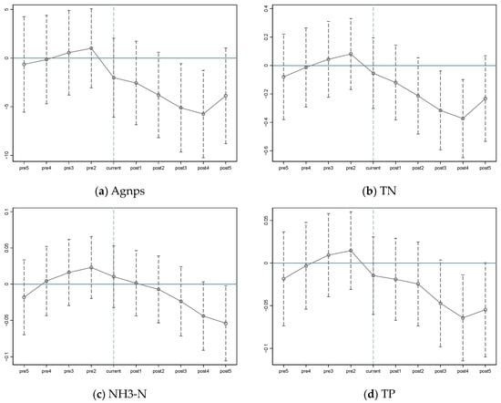
Figure 2.
Parallel trend test.
4.2.2. Placebo Test
- (1)
- Time–placebo test
To ensure that changes in agricultural pollution emissions within provinces are not merely due to changes over time, we create a fictional policy variable that does not actually exist. This allows us to confirm the causal link between the TRS policy and Agnps emissions. Using this method, we can more precisely measure the policy’s effects by accounting for factors that change over time and might otherwise skew our analysis. The construction is carried out as follows: (1) The policy period is defined as 2014–2021, and the variable is created accordingly. Given that the Chinese government proposed the TRS policy in 2014 but not all provinces immediately responded and implemented it, if the coefficient of this dummy variable remains significant, it would cast doubt on the credibility of the previous estimation results. Conversely, if the coefficient is not significant, it would validate the robustness of the findings presented in this study. (2) For each province that has implemented the policy, the time point of the policy is advanced by one year (), lagged by one year (), and lagged by two years (), respectively. When we shift the policy’s start date forward, essentially including data that were supposed to be in the control group in the experimental group instead, we anticipate that the policy’s impact will be reduced or even eliminated. On the other hand, if we push back the timeline of the policy, even if the size of the experimental group becomes smaller, the policy effect should still be evident, and the calculated coefficients should remain statistically significant. The estimation results from Table 4 reveal that the estimated coefficients for and are not significant, indicating that there is no systematic temporal difference in Agnps between provinces that have implemented the policy and those that have not. Meanwhile, the coefficients for and remain significantly negative, suggesting that the policy has a clear effect and exhibits a degree of persistence. This further validates the robustness of the findings presented in this study.
Table 4.
Time–placebo Test.
- (2)
- Individual placebo test
To more firmly establish a causal link between the TRS policy and the decrease in Agnps and to reduce the impact of other unseen factors on our findings, we conducted a placebo test using the approach suggested by Lu et al., (2017) [38]. Specifically, this paper randomly selects a subset of provinces from the sample of 30 provinces as the treatment group and re-estimates the benchmark model, thereby obtaining an estimated coefficient for a fictitious TRS policy variable. Furthermore, the aforementioned process is repeated 500 times to obtain 500 regression coefficient estimates for the core explanatory variable, along with their p-values. A kernel density distribution and a p-value combination plot are then created, as illustrated in Figure 3. As can be seen in Figure 3a, the coefficients based on the random samples follow a normal distribution and are centered around zero. Additionally, the majority of the regression coefficients have p-values greater than 0.01. The black dashed line represents the estimated coefficient from the benchmark model mentioned earlier, which is notably different from the mean of the kernel density distribution. Consequently, the policy effects of the TRS are not attributable to other random and unobservable factors, thereby confirming the reliability of the benchmark regression results presented in this study. Additionally, Figure 3b–d, which respectively considers TN, NH3-N, and TP as the dependent variables, shows a distribution of p-values and regression coefficients consistent with Figure 3a. This further substantiates the robustness of the policy effects.
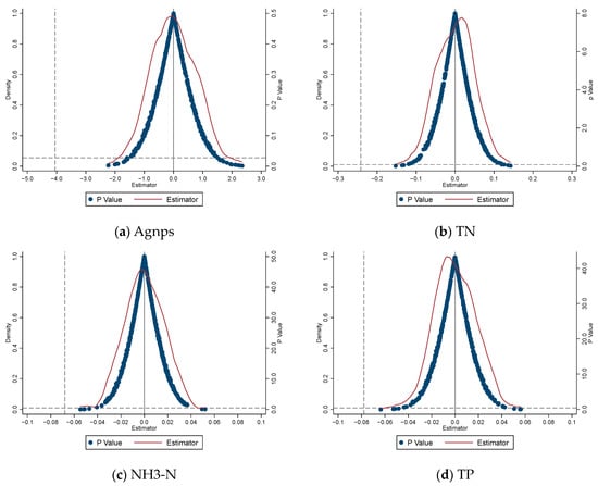
Figure 3.
Individual placebo test.
4.2.3. Other Robustness Tests
1. Adjustment of the sample time frame. On 1 January 2019, the revised “Rural Land Contracting Law of the People’s Republic of China” was officially implemented, legally establishing the separation of rural land ownership rights, contracting rights, and management rights. To prevent any interference from this event on the results of this study, the approach taken by Zhou (2022) was followed by excluding the samples from 2019 and onwards; additionally, samples prior to 2014 were also excluded [12]. As shown in columns (1) and (2) of Table 5, the coefficient of the policy dummy variable remains significantly negative, indicating that the results are still robust.
Table 5.
Other robustness tests.
2. Excluding municipalities. To avoid any bias in our results due to differences in size between municipalities directly governed by the central government and regular provinces, this study leaves out the samples from those municipalities in our regression analysis. The results in the third column of Table 5 show a significantly negative coefficient at the 1% level, reinforcing this study’s robust empirical findings.
3. Controlling other policies during the same period. In order to avoid the interference of other provincial-level policies that may affect the estimation results of Agnps, carbon trading pilot (CTP) policies and central environmental protection inspections (CEPI) in the same period were collected. The carbon trading pilot program aims to drive down carbon emissions through market-based approaches, supporting a shift to a low-carbon economy. This effort is key to meeting international pledges for “carbon peak” and “carbon neutrality”. With agriculture being a major economic sector in China and contributing to the country’s overall carbon emissions, reaching these emission reduction targets will involve strategies such as optimizing crop planting, promoting the reuse of waste resources, and cutting back on traditional pesticide and fertilizer use. These changes are expected to have an impact on Agnps. The central environmental protection inspection aims to bolster the development of ecological civilization by addressing environmental pollution and ecological damage. It includes agriculture in its scope, ensuring that farming practices are subject to scrutiny. Additionally, the inspection’s intermittent sampling and accountability systems encourage local leaders to prioritize agricultural issues, which in turn can impact agricultural pollution. To mitigate the potential impact of the above policies, the policy dummy variables of carbon trading pilot and central environmental protection inspection are added to the baseline model, and the results are shown in column (4) of Table 5, which shows that the impact of the TRS policy on Agnps is still significantly negative, while the coefficients of the CTP and the CEPI are not significant.
4. Censoring. To avoid extreme values affecting the estimation results, column (5) of Table 5 is bilaterally shaded at the 1% quantile, and the regression results are found to be still significant.
4.2.4. PSM-DID
Recognizing that there might be inherent differences between provinces where the policy is in place and those where it is not, we need to account for potential selection bias in how we define the experimental group. Alternatively, the propensity score matching (PSM) method can identify a control group that closely matches the experimental group in terms of characteristics. This helps to minimize internal disturbances by meeting the equilibrium assumption before applying the difference-in-differences approach to evaluate policy impacts. Two matching methods are used: radius matching and kernel matching. In Table 6, (1) and (2) show the results of radius matching estimation, while (2) adds control variables to (1), and the coefficients are all found to be significant at the 1% level of significance; columns (3) and (4) show the results of kernel matching estimation with no control variables added versus its results with the addition of control variables, respectively, and the estimated coefficients are all significant and very robust.
Table 6.
PSM-DID test.
5. Mechanism Analysis
This section further explores the impact mechanism of the TRS land reform on Agnps. We can anticipate that the larger the scale of agricultural operations or the agricultural economy in a province, the more significant the impact of the policy will be in curbing Agnps. On the basis of the benchmark model, the following settings are made:
where is the mechanism variable and the rest of the variables have the same meaning as in model (1).
Scale of agricultural operations. As another institutional innovation in rural reform after the household contract responsibility system, the TRS reform is a reinforcement of the property rights attribute of land and leads to the gradual extension of the function of land from the traditional functions of employment and security to the functions of income, property, and capital. The implementation of the TRS will revitalize rural land transfer and, at the same time, will also help the moderate and large-scale operation of agriculture and rationalize the allocation of factors of production such as land, capital, and labor. The interaction term and its separate terms of the policy variables of land transfer area and TRS are brought into the regression equation, and the results are shown in Table 7(1). The coefficients of the interaction term are significant at the 1% level of significance. Moreover, the coefficients of the interaction term and the policy dummy variable are both negative, indicating that the higher the degree of land transfer, the greater the inhibition effect of TRS on Agnps in the provinces.
Table 7.
Regression results with the addition of the cross-multiplication term.
Scale of the agricultural economy. For a long time, China has struggled with a structural imbalance in employment, with an oversupply of labor in rural areas and far more people working in agriculture than in industry or services. In addition to the household registration system, the rural land system has also been a key factor contributing to this employment imbalance [39]. The focus of this paper’s land system reform is to unlock the potential of rural land management rights, and by doing so, it encourages the most effective use and distribution of land resources, thereby driving a more market-based approach to the allocation of rural land [40]. As agriculture evolves, it transitions from a heavy reliance on labor to a mix of technology and fewer manual workers. However, China’s agricultural modernization is still in its early stages. In the initial phase of technology adoption, technology implementation often needs a certain level of labor support. Consequently, during this period, the growth of the agricultural economy is closely tied to the number of people employed in primary industries [41]. The interaction term of and and its separate terms are brought into the main regression, and the results are shown in Table 7(2). The coefficient of the interaction term is significantly negative at the 1% significance level, and the coefficient of the policy dummy variable is also negative, i.e., the moderating variable strengthens the negative relationship between the policy and the explanatory variables. This indicates that after the implementation of the TRS, the inhibition effect of Agnps is more significant in areas with more people in the primary industry than in areas with fewer people in the primary industry.
6. Heterogeneity
Whether it is a major food-producing region. Considering the long-standing cultural differences among regions and the varying natural resource endowments, agricultural practices in different provinces exhibit distinct characteristics. For instance, provinces with extensive plains are well-suited for large-scale cultivation, while those with a high proportion of hilly and mountainous terrain face challenges in agricultural development. In this part, according to the distribution of China’s major food-producing areas, the sample is divided into two groups, with 13 provinces located in the main grain-producing areas, such as Heilongjiang, Henan, and Shandong, as one group and the rest of the provinces as one group, to explore whether there is any difference in the influence mechanism mentioned above. The regression results are shown in Table 8. Columns (1) and (4) show the effects of TRS on Agnps in the major food-producing provinces and in non-major food-producing areas, respectively, and both are found to be significantly negative but more significant in the major food-producing areas; columns (2) and (3) show the mechanism we have discussed for food-producing provinces; while columns (5) and (6) indicate that the cross-multiplier terms are still significant in food-producing regions, with larger absolute values. However, the coefficients in non-food-producing regions are not significant, suggesting that the mechanism described above does not hold in those areas.
Table 8.
Heterogeneity analysis of whether or not they are located in major food-producing areas.
In summary, the TRS policy has a more pronounced effect on reducing Agnps in the major food-producing regions. This is due to two main reasons: first, these provinces have a larger agricultural economy and more agricultural workers, which enables them to implement central government policies more effectively. Second, the agricultural structure in these regions is more focused on crop cultivation, which is more likely to lead to higher levels of Agnps. Therefore, they are more sensitive to the pollution reduction effects of the TRS policy. In contrast, in non-food-producing regions, while the policy still has some effect on reducing Agnps, it is more difficult to achieve this through land transfer and employment in the primary industry. This is because the proportion of crop cultivation in these regions is not as high, and their smaller agricultural economies make them less inclined to spontaneously respond and implement the TRS policy compared to the food-producing regions.
7. Conclusions and Policy Implications
7.1. Conclusions
The reform of China’s land system has been a continuous and evolving process for the government since the country’s establishment. It not only fulfills the traditional concept of “land for the cultivator” but also plays a crucial role in balancing the relationship between urban and rural areas. The TRS, which separates ownership, contracting, and management of rural land, is a tangible example of the ongoing enhancement of the land system. Against this background, this paper conducts a case study, utilizing provincial panel data from 2011 to 2021 to analyze the impact of the TRS on Agnps and its mechanisms. This study found that (1) the TRS in all provinces of China has a significant inhibiting effect on the emission of Agnps as well as on the emission of TN, NH3-N, and TP pollutants. (2) The policy effect of TRS on pollution reduction is more obvious in provinces with a higher degree of agricultural scale and a larger agricultural economy. (3) Heterogeneity analysis shows that the TRS policy has a stronger effect on reducing Agnps in major food-producing provinces compared to those in non-food-producing regions. Moreover, the two pathways proposed in our hypothesis are not observed in the latter group.
7.2. Policy Implications
Based on the analysis of the above findings, several policy recommendations can be drawn, as follows: (1) Encourage large-scale agricultural operations and give full play to the positive effects of land transfer. The TRS reform has curbed the emission of Agnps, and the large-scale operation of agriculture serves as one of the mechanisms. Since accelerated land transfer is a prerequisite for large-scale agricultural production, policymakers should consider how to improve the existing land transfer market transaction system to protect the rights and interests of land contract operators. (2) Accelerate the cultivation of new business entities and increase the scale of the agricultural economy. Unlike the agricultural operations of developed countries, China’s large-scale agriculture has just started, and the number of institutions that can provide modern agricultural socialization services is still relatively small, so it is difficult for advanced seed cultivation, grain storage, agricultural product processing, and other technologies to fully cover the rural areas. Therefore, it is necessary to strengthen the cultivation of high-quality farmers, family farms, farmers’ cooperatives, and other new business entities to improve the efficiency of agricultural production and the level of modernization of agriculture, and then grow the agricultural economy. (3) Encourage the application of agricultural technology and improve the level of green agricultural production. The application of agricultural technology is an important reason why large-scale production can reduce Agnps emissions. China’s current mode of agricultural production is still mostly traditional, and its level of mechanization lags behind that of developed countries, so the government should provide certain subsidies to encourage the use of agricultural machinery and organic fertilizers.
Against the backdrop of global Agnps worsening without clear causes, this case study of China’s TRS land reform demonstrates that a well-defined land ownership system and scaled agricultural operations can significantly suppress Agnps, offering a reference for addressing Agnps worldwide. However, the heterogeneity of policies across different countries is also a critical issue that requires careful consideration. For instance, in less developed countries where land tenure is not entirely clear, it is necessary to approach the issue from the perspective of improving and optimizing institutional frameworks. These countries could adopt pilot policies similar to those implemented in China, adjusting and refining the policies in practice to align with local culture and farmers’ perspectives. Starting with small-scale pilots and gradually expanding to larger areas, this approach can lead to the green and sustainable development of agriculture. On the other hand, in developed countries where land tenure is well-defined and agricultural scaling is already relatively advanced, the focus can be on the research and application of green agricultural technologies.
Author Contributions
D.Y.: conceptualization, formal analysis, software, and writing—original draft and review. X.H.: data curation, formal analysis, visualization, and writing—review and editing. Z.W.: writing—review and editing. H.C.: conceptualization, methodology, and writing—review and editing. All authors have read and agreed to the published version of the manuscript.
Funding
This research was funded by Xihua University Graduate Student Science and Innovation Competition Project “Study on the Policy Support System for Migrant Workers Returning to Their Hometowns for Entrepreneurship and Employment in the Old Revolutionary Areas of Sichuan under the Perspective of Rural Revitalization”.
Institutional Review Board Statement
Not applicable.
Data Availability Statement
The data used in this study are publicly available, data sources are indicated in the text.
Conflicts of Interest
All authors certify that they have no affiliations with or involvement in any organization or entity with any financial interest or non-financial interest in the subject matter or materials discussed in this manuscript.
References
- Corwin, D.L.; Vaughan, P.J.; Loague, K. Modeling Nonpoint Source Pollutants in the Vadose Zone with GIS. Environ. Sci. Technol. 1997, 31, 2157–2175. [Google Scholar] [CrossRef]
- Napoletano, P.; Guezgouz, N.; Benradia, I.; Benredjem, S.; Parisi, C.; Guerriero, G.; De Marco, A. Non-Lethal Assessment of Land Use Change Effects in Water and Soil of Algerian Riparian Areas along the Medjerda River through the Biosentinel Bufo spinosus Daudin. Water 2024, 16, 538. [Google Scholar] [CrossRef]
- Feng, T.; Xiong, R.; Huan, P. Productive use of natural resources in agriculture: The main policy lessons. Resour. Policy 2023, 85, 103793. [Google Scholar] [CrossRef]
- Qin, G.; Niu, Z.; Yu, J.; Li, Z.; Ma, J.; Xiang, P. Soil heavy metal pollution and food safety in China: Effects, sources and removing technology. Chemosphere 2021, 267, 129205. [Google Scholar] [CrossRef]
- Ma, W.; Pan, Y.; Sun, Z.; Liu, C.; Li, X.; Xu, L.; Gao, Y. Input Flux and the Risk of Heavy Metal(Loid) of Agricultural Soil in China: Based on Spatiotemporal Heterogeneity from 2000 to 2021. Land 2023, 12, 1240. [Google Scholar] [CrossRef]
- Xu, J.; Cui, Z.; Wang, T.; Wang, J.; Yu, Z.; Li, C. Influence of Agricultural Technology Extension and Social Networks on Chinese Farmers’ Adoption of Conservation Tillage Technology. Land 2023, 12, 1215. [Google Scholar] [CrossRef]
- Chen, C.; Woods, M.; Chen, J.; Liu, Y.; Gao, J. Globalization, state intervention, local action and rural locality reconstitution—A case study from rural China. Habitat Int. 2019, 93, 102052. [Google Scholar] [CrossRef]
- Xiong, W.; Wang, Y. Contemporary peasant collectives: A discussion of a four-dimensional analytical framework. Soc. Dev. Res. 2015, 2, 62–85+243. [Google Scholar]
- Zang, Z.; Zhou, G.; Geng, Y.; Li, H.; Zhao, S.; Liu, Z. Changes of land system in ancient China under the perspective of materialistic view of history. China Soc. Sci. 2020, 1, 153–203+207–208. [Google Scholar]
- Qu, Y.; Li, Y.; Zhao, W.; Zhan, L. Does the rural housing land system reform model meeting the needs of farmers improve the welfare of farmers? Socio-Econ. Plan. Sci. 2023, 90, 101757. [Google Scholar] [CrossRef]
- Li, K.; Liu, C.; Ma, J.; Ankrah Twumasi, M. Can Land Circulation Improve the Health of Middle-Aged and Older Farmers in China? Land 2023, 12, 1203. [Google Scholar] [CrossRef]
- Zhou, L.; Shen, K. The income-generating effects of rural land system reform in China: Empirical evidence from the “three rights separation”. Econ. Res. 2022, 57, 141–157. [Google Scholar]
- Yan, J.; Yang, Y.; Xia, F. Subjective land ownership and the endowment effect in land markets: A case study of the farmland “three rights separation” reform in China. Land Use Policy 2021, 101, 105137. [Google Scholar] [CrossRef]
- Gong, M.; Li, H.; Elahi, E. Three Rights Separation reform and its impact over farm’s productivity: A case study of China. Land Use Policy 2022, 122, 106393. [Google Scholar] [CrossRef]
- Zhang, X.; Hu, L.; Yu, X. Farmland Leasing, misallocation Reduction, and agricultural total factor Productivity: Insights from rice production in China. Food Policy 2023, 119, 102518. [Google Scholar] [CrossRef]
- Xu, Y.; Huang, X.; Bao, H.X.H.; Ju, X.; Zhong, T.; Chen, Z.; Zhou, Y. Rural land rights reform and agro-environmental sustainability: Empirical evidence from China. Land Use Policy 2018, 74, 73–87. [Google Scholar] [CrossRef]
- Chen, Y.; Wang, H.; Cheng, Z.; Smyth, R. Early-life experience of land reform and entrepreneurship. China Econ. Rev. 2023, 79, 101966. [Google Scholar] [CrossRef]
- Gao, J.; Liu, Y.; Chen, J. China’s initiatives towards rural land system reform. Land Use Policy 2020, 94, 104567. [Google Scholar] [CrossRef]
- Wang, Q.; Zhang, X. Three rights separation: China’s proposed rural land rights reform and four types of local trials. Land Use Policy 2017, 63, 111–121. [Google Scholar] [CrossRef]
- Gong, M.; Zhong, Y.; Zhang, Y.; Elahi, E.; Yang, Y. Have the new round of agricultural land system reform improved farmers’ agricultural inputs in China? Land Use Policy 2023, 132, 106825. [Google Scholar] [CrossRef]
- de Janvry, A.; Emerick, K.; Gonzalez-Navarro, M.; Sadoulet, E. Delinking Land Rights from Land Use: Certification and Migration in Mexico. Am. Econ. Rev. 2015, 105, 3125–3149. [Google Scholar] [CrossRef]
- Gao, X.; Shi, X.; Fang, S. Property rights and misallocation: Evidence from land certification in China. World Dev. 2021, 147, 105632. [Google Scholar] [CrossRef]
- Galiani, S.; Schargrodsky, E. Property rights for the poor: Effects of land titling. J. Public Econ. 2010, 94, 700–729. [Google Scholar] [CrossRef]
- Goldstein, M.; Houngbedji, K.; Kondylis, F.; O’Sullivan, M.; Selod, H. Formalization without certification? Experimental evidence on property rights and investment. J. Dev. Econ. 2018, 132, 57–74. [Google Scholar] [CrossRef]
- Zhang, Z.; Zhao, H. The dilemma of new agricultural management main body and its institutional mechanism innovation. Reform 2013, 2, 78–87. [Google Scholar]
- Fang, D.; Guo, Y. Induced Agricultural Production Organizations under the Transition of Rural Land Market: Evidence from China. Agriculture 2021, 11, 881. [Google Scholar] [CrossRef]
- Chen, C. Technology adoption, capital deepening, and international productivity differences. J. Dev. Econ. 2020, 143, 102388. [Google Scholar] [CrossRef]
- Foster, A.D.; Rosenzweig, M.R. Are There Too Many Farms in the World? Labor-Market Transaction Costs, Machine Capacities and Optimal Farm Size; National Bureau of Economic Research: Cambridge, MA, USA, 2017. [Google Scholar] [CrossRef]
- Zhou, N.; Cheng, W.; Zhang, L. Land rights and investment incentives: Evidence from China’s Latest Rural Land Titling Program. Land Use Policy 2022, 117, 106126. [Google Scholar] [CrossRef]
- Khan, Z.A.; Koondhar, M.A.; Tiantong, M.; Khan, A.; Nurgazina, Z.; Tianjun, L.; Fengwang, M. Do chemical fertilizers, area under greenhouses, and renewable energies drive agricultural economic growth owing the targets of carbon neutrality in China? Energy Econ. 2022, 115, 106397. [Google Scholar] [CrossRef]
- Duan, W.; Jiang, M.; Qi, J. Agricultural certification, market access and rural economic growth: Evidence from poverty-stricken counties in China. Econ. Anal. Policy 2024, 81, 99–114. [Google Scholar] [CrossRef]
- Wu, A.; Elahi, E.; Cao, F.; Yusuf, M.; Abro, M.I. Sustainable grain production growth of farmland–A role of agricultural socialized services. Heliyon 2024, 10, e26755. [Google Scholar] [CrossRef] [PubMed]
- Murtisari, A.; Irham, I.; Mulyo, J.H.; Waluyati, L.R. Do poor farmers have entrepreneurship skill, intention, and competence? Lessons from transmigration program in rural Gorontalo Province, Indonesia. Open Agric. 2022, 7, 794–807. [Google Scholar] [CrossRef]
- Lu, H.; Chen, Y.; Luo, J. Development of green and low-carbon agriculture through grain production agglomeration and agricultural environmental efficiency improvement in China. J. Clean. Prod. 2024, 442, 141128. [Google Scholar] [CrossRef]
- Liu, Y.; Ji, Y.; Shao, S.; Zhong, F.; Zhang, N.; Chen, Y. Scale of Production, Agglomeration and Agricultural Pollutant Treatment: Evidence From a Survey in China. Ecol. Econ. 2017, 140, 30–45. [Google Scholar] [CrossRef]
- Liu, Y.; She, Y.; Liu, S.; Lan, H. Supply-shock, demand-induced or superposition effect? The impacts of formal and informal environmental regulations on total factor productivity of Chinese agricultural enterprises. J. Clean. Prod. 2022, 380, 135052. [Google Scholar] [CrossRef]
- Huang, Y.; Gan, J.; Liu, B.; Zhao, K. Environmental policy and green development in urban and rural construction: Beggar-thy-neighbor or win-win situation? J. Clean. Prod. 2024, 446, 141201. [Google Scholar] [CrossRef]
- Lu, Y.; Tao, Z.; Zhu, L. Identifying FDI spillovers. J. Int. Econ. 2017, 107, 75–90. [Google Scholar] [CrossRef]
- Xu, X.; Jin, Z. Impact of Return Migration on Employment Structure: Evidence from Rural China. J. Asian Econ. 2024, 91, 101697. [Google Scholar] [CrossRef]
- Li, J.; Xiong, C.; Cai, J. Starting a new milestone of urban-rural land property rights homologation and market-oriented reform of resource allocation. Manag. World 2020, 36, 93–105+247. [Google Scholar] [CrossRef]
- Li, L.; Khan, S.U.; Guo, C.; Huang, Y.; Xia, X. Non-agricultural labor transfer, factor allocation and farmland yield: Evidence from the part-time peasants in Loess Plateau region of Northwest China. Land Use Policy 2022, 120, 106289. [Google Scholar] [CrossRef]
Disclaimer/Publisher’s Note: The statements, opinions and data contained in all publications are solely those of the individual author(s) and contributor(s) and not of MDPI and/or the editor(s). MDPI and/or the editor(s) disclaim responsibility for any injury to people or property resulting from any ideas, methods, instructions or products referred to in the content. |
© 2024 by the authors. Licensee MDPI, Basel, Switzerland. This article is an open access article distributed under the terms and conditions of the Creative Commons Attribution (CC BY) license (https://creativecommons.org/licenses/by/4.0/).