Computational Fluid Dynamics Model with Realistic Plant Structures to Study Airflow in and around a Plant Canopy on a Cultivation Shelf in a Plant Factory with Artificial Light

Abstract

Airflow plays a crucial role in plant growth because it supplies CO₂, O₂, and energy to plants in a plant factory with artificial light (PFAL). Therefore, understanding how various factors affect airflow in and around a plant canopy is essential. In this study, we developed a computational fluid dynamics (CFD) model with realistic plant structures created using structure-from-motion imaging to investigate airflow in and around a plant canopy. The averages of the absolute percentage errors of simulated air velocity in three conditions were 6.7%, 10.1%, 12.7%, respectively. The simulated and measured air velocities agreed well, confirming the accuracy of the developed CFD model. The effects of inflow velocities and plant canopy structures on the airflow in and around the plant canopy were analysed using the validated CFD model. The inflow velocities significantly decreased stagnant zones (from 62.4% to 7.2%) and increased the airflow uniformity in and around the plant canopy. A staggered layout of the plant canopy slightly decreased stagnant zones (from 16.4% to 13.2%) and increased the airflow uniformity. The airflow in and around the plant canopy was further inhibited by a large plant structure. This CFD model provided a basis for improving the airflow status in and around a plant canopy in a PFAL.

1. Introduction

Currently, agricultural production faces numerous challenges, including population growth, urbanisation, unusual weather patterns, uneven distribution of natural resources, and food security [1]. A plant factory with artificial light (PFAL) or vertical farm is considered a viable solution in which environmental factors, such as temperature, humidity, and light, can be optimally controlled, and the facilities can be built at any location [2]. In addition, it achieves year-round crop production [3] and provides high-quality plants [4]. In the PFAL, airflow significantly influences the microclimate in and around a compact plant canopy [5,6] depending on the convection transfer of heat and mass [7]. It determines factors such as leaf and air temperatures [8], humidity, and carbon dioxide concentration. Low airflow cannot mitigate uneven temperature gradients from lamps in the vertical direction or non-homogeneous gas concentrations in the plant canopy. Meanwhile, an appropriate range of airflow (0.1–1.3 m s⁻¹) promoted photosynthesis and transpiration rates in plants because it increases gas exchange rates through a high gas gradient and decreasing boundary layer resistance between plants and the surrounding atmospheres [9]. Airflow patterns in and around a plant canopy are affected by airflow controls such as inflow velocity and direction. Previous studies have demonstrated that appropriate airflow control can influence plant growth [10,11], improve the photosynthesis and transpiration rates of plants [12,13], and prevent lettuce tipburn [14,15,16]. In addition, different layouts, planting densities, and leaf shapes and angles [17] affect airflow in and around the plant canopy because plant structures are correlated with airflow patterns, owing to skin friction and the form drag of plants [18]. However, knowledge regarding the airflow passing through a plant canopy remains limited. To effectively improve the airflow in and around a plant canopy, the ways in which various elements such as inflow velocity and plant canopy structures directly affect airflow patterns and which elements play a dominant role must be understood.

Studies on flow phenomena are typically conducted using experimental measurements and computational fluid dynamics (CFD). However, experimental measurements are expensive and time-consuming. Owing to the limited number of measured points, it is challenging to obtain the entire airflow information. In addition, the accuracy of measurements is affected by the inevitable interference of sensors with airflow [19]. Therefore, quantifying the complicated effects of various factors on airflow in and around a plant canopy is almost impossible. CFD involves the use of numerical methods to solve fluid flow problems and simulate complex physical phenomena with reasonable accuracy [20]. In greenhouses, CFD is an effective and well-established tool for analysing ventilation phenomena [21,22] and climate distribution [23,24]. Several studies have optimised the airflow in an indoor plant factory using a CFD approach [25,26,27,28]. Some studies have focused on improving the airflow around plants using the CFD method. Okayama et al. simulated the airflow near lettuce replicas under different multi-fan systems using cubic lettuce geometry models [29]. Zhang et al. improved the airflow uniformity over a plant canopy through a vertical airflow design, considering the plant canopy surface to be a rough wall [30]. Similarly, Fang et al. optimized the airflow on the surface of a plant canopy using a horizontal airflow and treating the plant canopy as a porous medium model [31]. In addition, some studies have enhanced the climate uniformity of plant canopies using a CFD model by setting localised air supply on each shelf [32,33,34,35].

In most CFD research, plants were modelled as an implicit porous medium with cuboidal or spherical geometries in greenhouses [36,37], orchards [38,39], and forest areas [40,41]. However, simulating detailed airflow patterns in and around plants using this method is challenging because of the lack of plant structural descriptions. Recently, a few studies have utilised the explicit geometry of trees and shrubs to estimate the effect of plants on flow fields using CFD models [42,43]. Detailed flow characteristics can be captured using a CFD model with an explicit geometry of the plants. These previous studies targeted plant growth in external environments, such as forest areas and street canyons. Leaves were simplified in these studies because of their complex plant structures. Leaves are important research objects in agricultural production. An explicit plant model can be established using direct and reverse modelling of plant components. Direct modelling requires the accurate measurement of each plant component. It is difficult to obtain a detailed description of plant structures (e.g., leaf textures) because of the high spatial complexity of plants [44,45]. Reverse modelling can directly extract structures from plants using a 3D scanner and a structure-from-motion (SFM) imaging technique. Several studies have estimated the light environment of plants using SFM [46,47,48].

The objective of the present study was to develop a CFD model with realistic plant structures to analyse the airflow in and around a plant canopy. In addition, the effects of various inflow velocities and plant canopy structures (e.g., days after sowing (DAS), arrangement, and leaf veins) on airflow were investigated. Therefore, a CFD model with a 3D realistic plant canopy was developed. Subsequently, experimental measurements were conducted to validate the 3D plant canopy and CFD models. Finally, the airflow in and around the plant canopy was systematically simulated and analysed under various inflow velocities and plant canopy structures. This study provides a foundational understanding for optimizing airflow in and around the plant canopy. It offers insights for designing more efficient airflow control in a cultivation shelf of PFALs.

2. Materials and Methods

2.1. Outline of CFD Model

We developed an accurate CFD model to simulate the airflow in and around a plant canopy. A commercial CFD program (Fluent, ver. 2021 R2, ANSYS Inc., Canonsburg, PA, USA) was used for the simulations. The simulation results were compared with the experimental results to validate the CFD model. The CFD model was designed to simulate a closed-type cultivation shelf used in the Research Unit for Closed-type Plant Production Systems at Matsudo Campus, Chiba University, Japan (Figure S1 and Figure 1). The conventional cultivation system in PFALs is an open-type but the modern closed-type cultivation shelf is designed to distribute a same temperature air from an air conditioner unit to each cultivation shelf (Figure S1).

The shelf was constructed using blackboards, and four LED lamps (LT-B4600T08-N, OHM ELECTRIC Inc., Saitama, Japan) were installed 0.4 m from the bottom wall. Air flowed through the holes into the cultivation space. Due to the non-uniform distribution of inlet velocity, the velocity was determined by measuring at 12 locations of the inlet area. Approximately 15 d after sowing (DAS), a soybean canopy, cultivated hydroponically in a container, was located at the centre of the chamber in the y-direction.

2.2. CFD Modelling

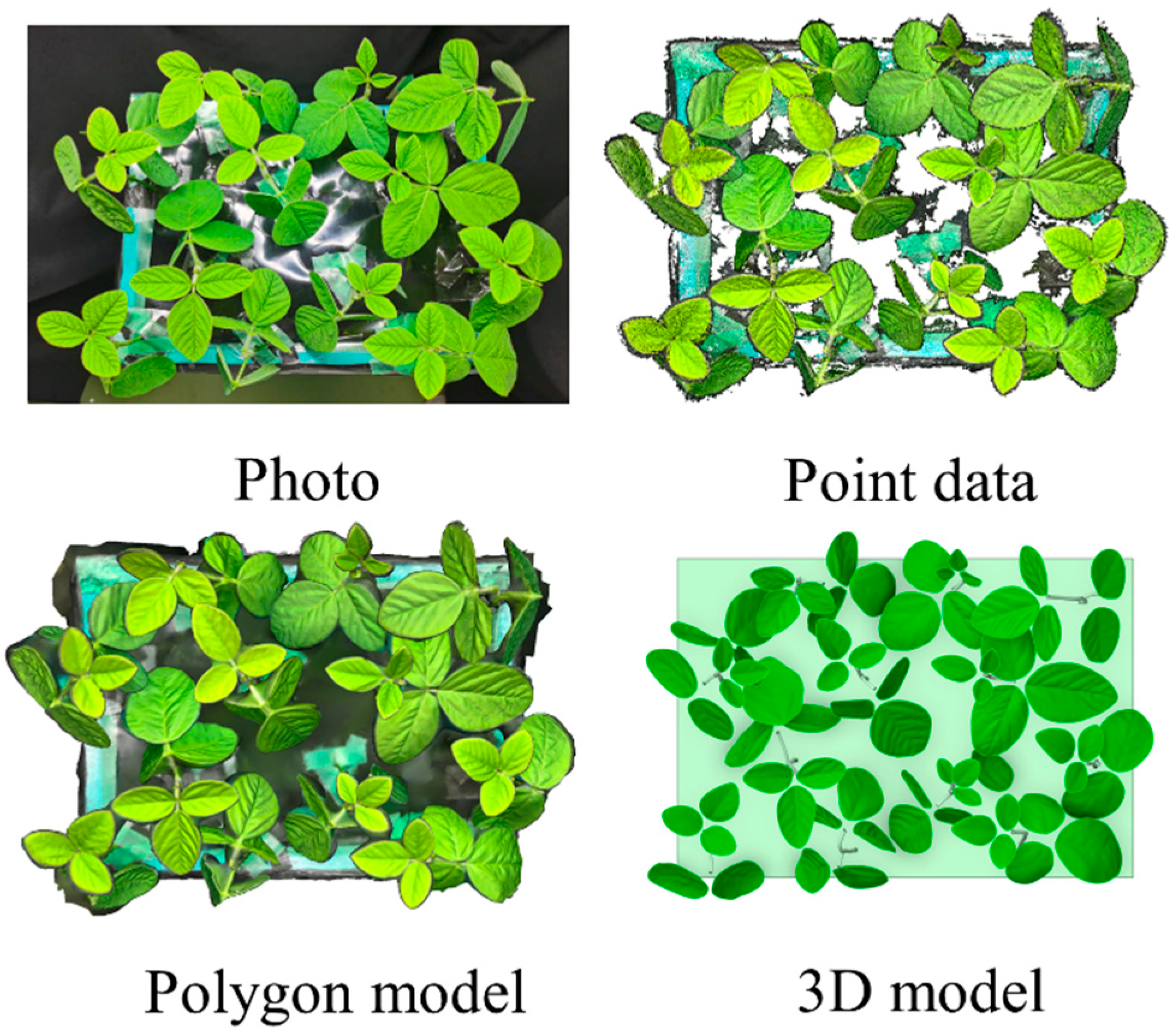
2.2.1. 3D Plant Canopy Models

Plant Material

We used vegetable soybean (Glycine max (L.) Merr., ‘Sirojisi’), also called edamame in Japanese, as a plant material [49]. Edamame is harvested and consumed at the immature developmental stage, which occurs when the seeds or pods become larger but do not turn yellow. Their cultivation period from germination is approximately 70 d and is shorter than those of fruit vegetables, such as strawberries and tomatoes. It is common for crops to be cultivated without agrichemicals in a PFAL; therefore, fresh and agrichemical-free edamame could be produced and made available to the market in the future [49,50].

3D Plant Canopy Model for CFD Model Validation

The 3D plant canopy model used for the CFD model validation was developed using a reverse modelling method. Plant structures were extracted using the structure-from-motion (SFM) imaging technique, which enabled us to obtain a realistic reconstructed model of plants [51]. This study focused on the leaves as a crucial research object; hence, the vegetative growth stage of soybeans was examined. Figure 2 shows the procedure for the 3D modelling of the soybean canopy. First, Metashape (ver.1.8.1, Agisoft LLC, St. Petersburg, Russia) was used to generate dense point clouds with photographs. Secondly, the point dataset was converted into a polygon model. Finally, a 3D plant canopy model was constructed using SpaceClaim (ver. 2021 R2, ANSYS Inc., Canonsburg, PA, USA) from the polyhedron model. The 3D plant canopy model included fine details of the leaves (veins). To reduce the calculation time and skew rate of grids, the stems of the 3D plant model were smoothed.

3D Plant Canopy Model for Case Simulations

A 17 DAS (days after sowing) and a 19 DAS 3D soybean model (Figure 3) were established using the method described in the above section. The 3D soybean without veins was reconstructed from the 3D 17 DAS soybean with veins using SpaceClaim. The 3D plant canopy models for the simulations were created by copying a single 3D soybean model (17 and 19 DAS), as shown in Figure 3.

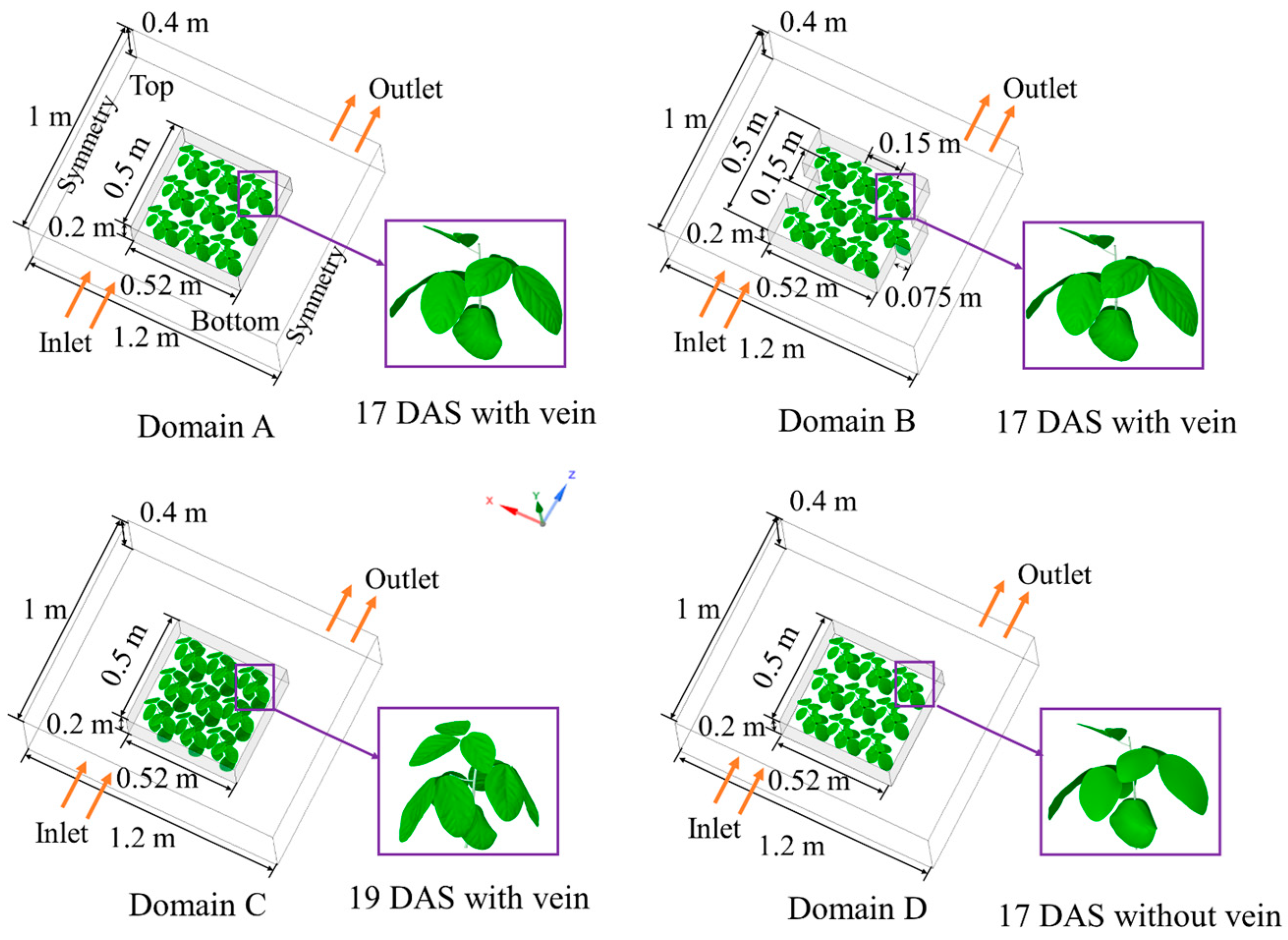
2.2.2. Simulation Domains

CFD Model Validation

Simulation domains for CFD model validation were created based on measurements of the shelf with and without plants (Figure 1). Computational domains were established using SpaceClaim (ver. 2021 R2) software. The simulation domain depicted in Figure 1A corresponds to condition 1, representing the scenario without soybeans. The simulation domains for conditions 2 and 3, illustrated in Figure 1B, incorporate soybean plants.

Case Simulations

Case simulations were used for studying the effect of inflow velocities and plant canopy structures (e.g., DAS, arrangement, and leaf veins) on airflow in and around plant canopies. In this study, we focused on six scenarios including different inlet air velocities, arrangements of plants, plant sizes, and leaf characteristics.

Table 1. Case settings.

	Inflow Velocity (m s−1)	Arrangement	DAS * (Day)	LAI (m−2 m−2)
Case 1	0.20	Square	17	1.00
Case 2	0.50	Square	17	1.00
Case 3	0.80	Square	17	1.00
Case 4	0.50	Stagger	17	1.00
Case 5	0.50	Square	19	1.40
Case 6	0.50	Square	17	0.99

* represents days after sowing.

summarises the settings of the six cases. Four simulation domains were created for each of the six cases (Figure 4). Domain A was used for Cases 1, 2, and 3 to analyse the airflow under different inflow velocities, because the difference among Cases 1, 2, and 3 was the inflow velocities (0.20, 0.50, and 0.80 m s⁻¹, respectively). Therefore, the simulation domain of Cases 1, 2, and 3 was the same. The inflow was in the z-direction. Domain B was used for Case 4 to analyse the airflow under different plant arrangements. The staggering distance of the middle row of plants was 0.075 m along the x-direction. In Domains A and B, the 3D plant canopy consisted of nine identical 17 DAS soybean plants (17 DAS 3D model in Figure 3). Domain C was used for Case 5 to examine the airflow alteration with different plant sizes. The 3D plant canopy included nine identical 19 DAS soybean plants (Figure 3). Domain D was used for Case 6 to analyse the effect of veins on the airflow. The 3D plant model without veins exhibited a smooth leaf surface (17 DAS 3D model without veins in Figure 3). In Table 1, LAI (m⁻² m⁻²) is defined as the ratio of one-sided leaf area to plant ground cover area (0.50 m × 0.52 m).

2.2.3. Transport Equations

The airflow in the computational domain was assumed to be a steady-state, incompressible, viscous, and three-dimensional flow. In this study, the detailed structures of turbulence were not important; therefore, the Reynolds-averaged Navier–Stokes (RANS) equation was applied to model the turbulence. The average mass and momentum equations are as follows:

$${\displaystyle \frac{\partial \rho }{\partial t}}+{\displaystyle \frac{\partial }{\partial x_i}}(\rho u_i)=0$$

(1)

$${\displaystyle \frac{\partial }{\partial t}}(\rho u_i)+{\displaystyle \frac{\partial }{\partial x_j}}(\rho u_i{u}_j)=-{\displaystyle \frac{\partial p}{\partial x_i}}+{\displaystyle \frac{\partial }{\partial x_j}}\left[\mu \left({\displaystyle \frac{\partial u_i}{\partial x_j}}+{\displaystyle \frac{\partial u_j}{\partial x_i}}-{\displaystyle \frac{2}{3}}{\delta }_{ij}{\displaystyle \frac{\partial u_i}{\partial x_i}}\right)\right]+{\displaystyle \frac{\partial }{\partial x_j}}\left(-\rho \overline{u_i^{\prime }{u}_j^{\prime }}\right)$$

(2)

where t is time (s); x_j is the coordinate in the j direction (m); u_i is the velocity component in the i direction (m s⁻¹); u_j is the velocity component in the j direction (m s⁻¹); ρ is the density (kg m⁻³); p is the pressure (Pa);${ u}_j^{\prime }$ is the fluctuating velocity component in the j direction (m s⁻¹);${ u}_i^{\prime }$ is the fluctuating velocity component in the i direction (m s⁻¹);$\rho \overline{u_i^{\prime }{u}_j^{\prime }}$ is Reynolds stresses; and δ_ij is Kronecker delta.

In several studies, a standard k-ε turbulent model was used to model the airflow through trees due to its robustness, economy, and reasonable accuracy [42,44]. However, the realisable k-ε turbulent model performed the best among all versions of the k-ε model for separated flows and flows with complex secondary flow features [52]. Therefore, it was employed to calculate two additional governing equations for the turbulent kinetic energy (k) and turbulent dissipation (ε) of RANS. Because the air temperature difference in the shelf is small (about 9 °C calculated by lamp temperature minus the bottom wall temperature of the shelf), the influence of buoyancy on air movements in the momentum equation was not considered.

Some assumptions relative to the leaves’ behaviour were considered as follows.

(1)

In contrast to the larger leaf area, the low thickness of leaves was ignored

(2)

The robust structure of the compact plant canopy presented a formidable barrier to airflow. Consequently, the minute vibrations of the leaves exert minimal influence on airflow and are therefore deemed insignificant.

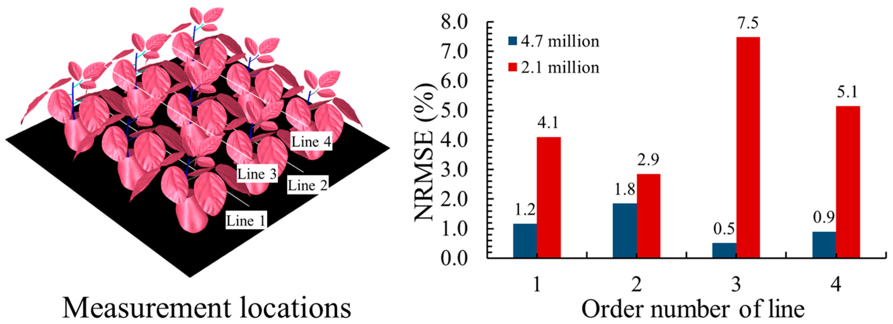
2.2.4. Meshes and Boundary Conditions

The meshes were generated using Fluent meshing (ver. 2021 R2, ANSYS Inc., Canonsburg, PA, USA). The mesh sizes in all the domains were resolved based on the minimum distance from the surface (y⁺). In the three models used for validation, the global mesh size was 0.01 m, and the mesh sizes of the containers, stems, and leaves were 0.004, 0.001, and 0.004 m, respectively. The computational grids of the CFD model without and with plants had 0.2 million cells and 1.3 million cells, respectively. The maximum values of skewness of meshes were 0.36 and 0.67 for CFD models without and with plants, respectively.

In the four domains, the global mesh size was 0.008 m. The mesh sizes of stems and leaves were 0.0006 and 0.004 m, respectively. The average cell count of Domains A, B, and D was 3.9 million, and the average maximum skewness value was 0.71. The cell count of Domain C was 5.7 million, and the maximum skewness was 0.67. The cells consisted of polyhedrons and hexahedrons. The surface meshes of plants for CFD model validation and case simulation are shown in Figure S2.

The independence of the grids was tested to avoid their influence on the simulation results. The results of the grid independence test for Case 2 are shown in Figure 5. Four air velocity profiles with three grid sizes, including 2.1 (coarse), 4.7 (medium), and 6.4 (fine) million, in a plant canopy were compared. The accuracies of the coarse and medium grids were evaluated using the normalised root mean squared error (NRMSE) [53]:

$$\mathrm{N}\mathrm{R}\mathrm{M}\mathrm{S}\mathrm{E}={\displaystyle \frac{3}{r^l-1}}\sqrt{{\displaystyle \frac{{\sum }_{i=1}^n{\left[y_1\left(i\right)-y_2\left(i\right)\right]}^2}{{\sum }_{i=1}^n{y_2\left(i\right)}^2}}}$$

(3)

where y₁(i) and y₂(i) are the prediction values for the coarse and medium grids, respectively; r = 2 is the grid change step which is recommended doubling or halving; l = 2 is the order of the numerical scheme which is determined by second-order discretisation schemes in solver setting; and n = 45 is the number of predicted values.

In the CFD model, the prediction values of the four lines in Figure 5 were collected, and the NRMSEs were compared between the coarse and medium grids, with the fine grid as the base. The NRMSEs of the coarse and medium grids were <10.0%. Both models produced satisfactory simulation results. However, 4.7 million cells (medium grid) were chosen for the superior accuracy in modelling the airflow.

The boundary condition settings were referred to [30,31,52,54]. The boundary conditions of the CFD models for these cases are summarised as follows: The inlet was set to the air velocity. The turbulence intensity was 5.0%, and the turbulent viscosity ratio was 10. The outlet was set to atmospheric pressure. The pressure at all boundaries of the atmospheric domains was set to zero. The bottom and plant surfaces were assumed to have non-slip walls. The other surfaces were symmetrical planes, in order to avoid the effects of walls on the airflow. The density and viscosity of air were 1.225 kg m⁻³ and 1.789 × 10⁻⁵ kg m⁻¹ s⁻¹, respectively.

2.2.5. Solver Settings

A pressure-based solver was used to solve the incompressible flows, and the SIMPLE algorithm was used for steady simulations to calculate the pressure–velocity coupling. A least-squares cell-based scheme of Fluent was used for the gradient terms. Second-order discretisation schemes were used for pressure, momentum, turbulent kinetic energy, and turbulent dissipation rate. Convergence was assessed by monitoring air velocity on specific locations in the flow field. The convergence criterion of residuals was set to 10⁻³ on the mass, momentum, and viscous terms. The solver settings were set with reference to the studies of [30,31,52,54]. Detailed settings for Fluent calculations are shown in Table S1. A computer (HP EliteDesk 800 G5, HP Japan Inc., Tokyo, Japan) with Intel i7-9700 (8 cores, 3.00 GHz, 64 GB RAM) was used to calculate the CFD model. The computing time for solving 5.7 million cells was 1 h using 2 solver processes over 200 iterations.

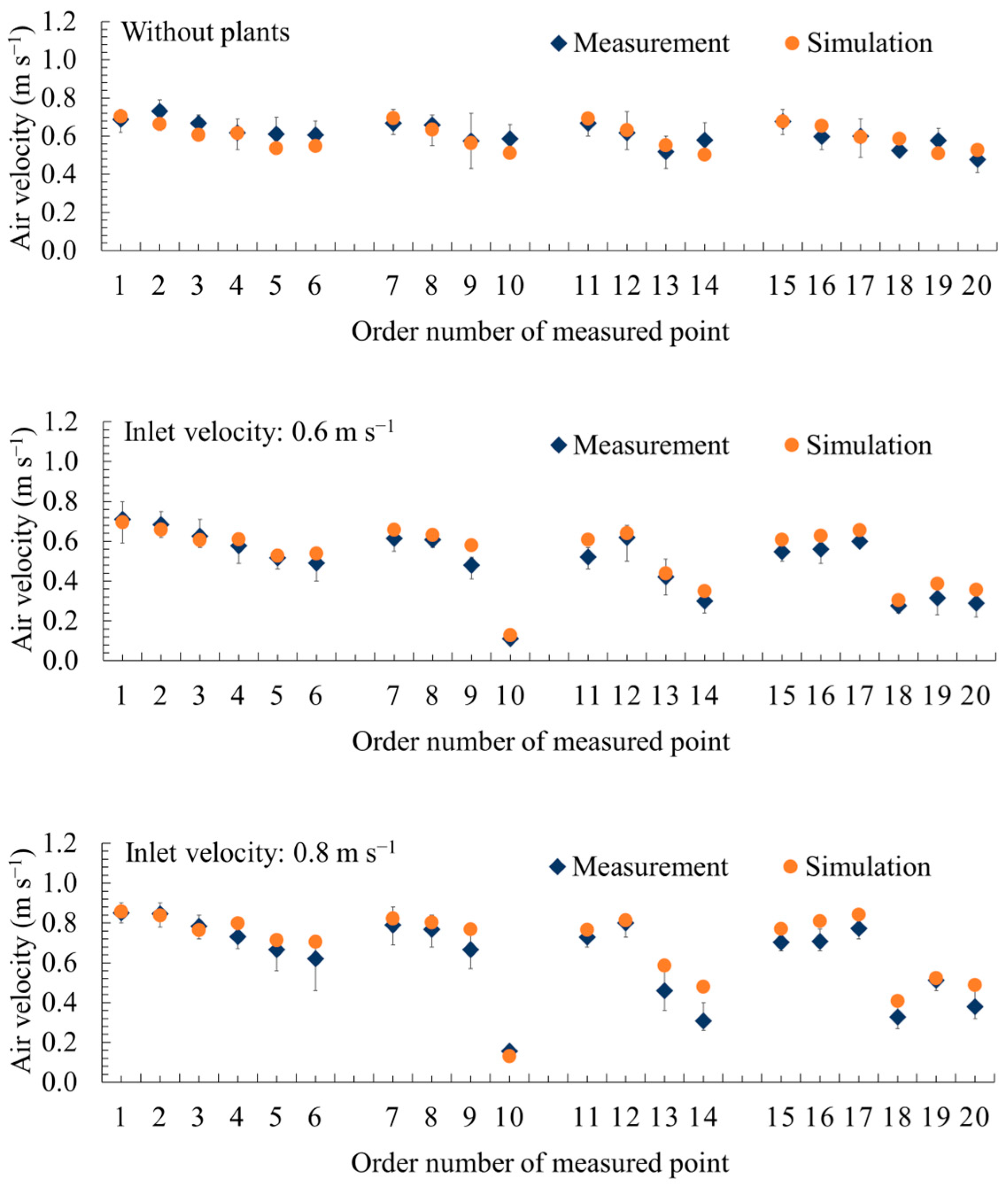
2.2.6. Experimental Measurements for CFD Model Validation

Three different measurements were performed by measuring air velocities on the shelf in Figure 1 (condition 1: under 0.6 m s⁻¹ inlet velocity without plants; conditions 2 and 3: under 0.6 and 0.8 m s⁻¹ inlet velocity with plants, respectively).

A hot-wire anemometer (CLIMOMASTER ^® MODEL 6501series, KANOMAX JAPAN Inc., Osaka, Japan) with a sensor (Range: 0.01–0.99 m s⁻¹, Accuracy: ±0.02 m s⁻¹ MODEL6543-21, KANOMAX JAPAN Inc., Osaka, Japan) was used to measure the air velocity. Air velocities at 20 different locations were measured in three different measurement conditions. The layout of the measurement points is shown in Figure 1. These data were necessary for validating the CFD model and were recorded every second for 15 s. The entire measured dataset was averaged for comparison with the simulation results.

2.2.7. Processing Results

The maximum air velocity (V_max); average air velocity (V_avg); percentages of cells (PC) with air velocity < 0.20, 0.20 ≤ air velocity ≤ 0.50, and air velocity > 0.50 m s⁻¹ and the coefficient of variation (CV) were used to assess overall airflow in and around the plant canopy (shown in Section 3.3). The uniformity of the airflow in and around the plant canopy was evaluated using CV, which was used in [30,32]. A high value indicated that the air velocity was non-uniform in and around the plant canopy. Stagnant zone distributions and normalised air velocity around leaves were used to visually analyse the airflow in and around the plant canopy. As pointed out by [55], air velocity ≥ 0.20 m s⁻¹ inside a plant canopy is better for photosynthesis. A zone where air velocity < 0.20 m s⁻¹ was defined as the stagnant zone. A low value indicates that the airflow in the canopy is not good for plant growth. The volumes with air velocity <0.20 m s⁻¹ in the plant canopy were calculated by using the ISO-volume method in CFD-Post. The visualised stagnant zone distributions are shown in Section 3.4. To clearly observe the airflow intensity around leaves, we calculated the wall shear stress (WSS) of leaves, which is the tangential force per unit area exerted by a flowing fluid on the wall. High WSS values are associated with a high local fluid velocity [56]. To facilitate a clear comparison of the airflow intensity around leaves for each case, we calculated normalized wall shear stress. The normalised WSS was calculated by WSS_n = (WSS − WSS_min)/(WSS_max − WSS_min), where WSS (Pa) was the calculated wall shear stress and WSS_max (Pa) and WSS_min (Pa) were the maximum and minimum WSS, respectively. The normalised air velocities around the leaves are shown in Section 3.5.

The V_max, V_avg, PC, stagnant zone distribution, and normalised air velocity around the leaves were calculated using CFD-Post (ver. 2021 R2, ANSYS Inc., Canonsburg, PA, USA). The CV was calculated using Python (ver. 3. 10).

3. Results and Discussion

3.1. 3D Plant Canopy Model Validation

The structure of the 3D plant canopy model resembled that of the real plant canopy (Figure 2). The location and structure of objects and the location of the camera at a scene were precisely estimated using the SFM imaging technique [57]. The leaf area of the real plant canopy was 0.09089 m², as measured using a leaf area meter (LI-3100, LI-COR Inc., Lincoln, NE, USA). The leaf area of the 3D plant canopy was 0.08311 m², as measured with SpaceClaim, which is slightly lower than 0.09089 m². The relative error (RE) of the 3D plant canopy was 8.6%. This discrepancy was caused by the rough point dataset of the leaf edges. This result indicates good agreement between the real and 3D plant canopies.

3.2. CFD Model Validation

Figure 6 compares the simulated air velocities with the measured air velocities at 20 locations in the three models. A remarkable agreement was observed between the simulated and measured air velocities in the CFD model without plants. The mean absolute error (MAE) and mean absolute percentage error (MAPE) of the CFD results were calculated for 20 locations to validate the CFD model [30,31]. The MAE and MAPE of the CFD model without plants were 0.04 m s⁻¹ and 6.7%, respectively. For the CFD model with plants, good agreement between the simulated and measured data was observed. The MAE and MAPE of the CFD model with plants were 0.04 m s⁻¹ and 10.1% at the 0.6 m s⁻¹ inlet and 0.06 m s⁻¹ and 12.7% at the 0.8 m s⁻¹ inlet, respectively. Most simulated values were within the maximum and minimum deviations of the measured mean values. The simulated values were slightly higher than the measured values. This discrepancy may be attributed to the underestimation of the leaf area in the 3D plant model. The error of simulation results may be caused by the imprecise setting of the inlet velocity, which was the non-uniform distribution, with a deviation of 4.9%. Furthermore, the experimental shelf was not completely airtight, leading to gas leakage and a lower measured air velocity. In addition, assuming smooth surfaces for both the shelf and containers may result in high simulated values. The current CFD model can predict air velocity in and around a plant canopy with satisfactory accuracy.

3.3. Airflow in and around a Plant Canopy in Case Simulations

Table 2. Airflow in and around the plant canopy in case simulations.

	Inflow Velocity (m s−1)	Vmax (m s−1)	Vavg (m s−1)	PC (<0.20 m s−1) (%)	PC (0.20–0.50 m s−1) (%)	PC (>0.50 m s−1) (%)	CV (%)
Case 1	0.2	0.33 ± 0.00	0.12 ± 0.00	62.3 ± 0.02	37.7 ± 0.02	0.0 ± 0.00	103.4 ± 0.00
Case 2	0.5	0.72 ± 0.00	0.36 ± 0.00	16.4 ± 0.03	58.2 ± 0.01	25.4 ± 0.02	91.1 ± 0.22
Case 3	0.8	1.21 ± 0.00	0.55 ± 0.00	7.2 ± 0.02	36.9 ± 0.03	56.0 ± 0.02	86.4 ± 0.25
Case 4	0.5	0.77 ± 0.00	0.37 ± 0.00	13.1 ± 0.10	59.5 ± 0.06	27.3 ± 0.04	87.1 ± 0.19
Case 5	0.5	0.79 ± 0.00	0.33 ± 0.00	25.6 ± 0.15	50.4 ± 0.06	24.0 ± 0.11	92.8 ± 0.12
Case 6	0.5	0.71 ± 0.00	0.36 ± 0.00	15.6 ± 0.00	58.9 ± 0.00	25.4 ± 0.00	77.1 ± 0.08

Each value represents the mean ± standard deviation (n = 5).

summarises the airflows in and around the plant canopy during the simulations with five different numbers of iterations. Each value represents the mean ± standard deviation. In Cases 1–3, with inflow velocities from 0.20 to 0.80 m s⁻¹, V_max and V_avg obviously increased from 0.33 and 0.12 m s⁻¹ to 1.21 and 0.55 m s⁻¹, respectively. The CV considerably decreased from 103.4% to 86.4%. PC (<0.20 m s⁻¹) considerably decreased from 62.3% to 7.2%, and PC (>0.50 m s⁻¹) obviously increased from 0.0% to 56.0%. This revealed that a high inflow velocity significantly increased the air velocity and improved uniformity in and around the plant canopy. Case 4, with a staggered layout, slightly increased the V_max and V_avg from 0.72 and 0.36 to 0.77 and 0.37 m s⁻¹, respectively, whereas the CV decreased from 91.1% to 87.1%. PC (<0.20 m s⁻¹) diminished with increased PC (0.20–0.50 m s⁻¹) and PC (>0.50 m s⁻¹). This finding indicates that the air velocity and uniformity in and around the plant canopy were increased by setting a staggered layout of the plants. Case 5, with a big plant geometry, had a high V_max of 0.79 m s⁻¹ and a low V_avg of 0.33 m s⁻¹. A rise in PC (<0.20 m s⁻¹) was obviously observed, from 16.4 to 25.6%, with descending PC (0.20–0.50 m s⁻¹) and PC (>0.50 m s⁻¹). The CV increased from 91.1 to 92.8%. These results indicate that the big plant geometry has negative effects on the air velocity and uniformity in and around the plant canopy. One reason for this could be that the LAI obviously increased as plant geometries became large (Table 1), resulting in a small plant-to-space ratio. Case 6 with a smooth leaf surface did not significantly affect V_max, V_avg, PC (0.20–0.50 m s⁻¹), or PC (>0.50 m s⁻¹). However, the CV decreased substantially from 91.1% to 77.1%, indicating that leaf veins had no significant effect on air velocity, but affected air uniformity. This may be because veins mainly increase skin friction in the plant canopy. Form drag affects the airflow in the canopy more than skin friction, owing to the angle between the leaf and airflow direction [18]. Leaf veins may affect air uniformity in and around the plant canopy due to the decreased V_max and PC (<0.20 m s⁻¹).

3.4. Stagnant Zone Distributions in Case Simulations

Figure 7 illustrates the distributions of the stagnant zones for the different simulation cases. Cases 1–3 show that the stagnant zones behind the plants were affected by the inflow velocities. The size of the stagnant zones decreased with increasing inflow velocity. However, they were still present in the second and third rows of the plant canopies. Stagnant zones were more evident on the leeward sides of the plants compared with other locations. This is because plants directly block the airflow rather than weaken it, causing a low-airflow zone on the leeward side of the plants [42]. The stagnant zones increased with the depth of the plant canopy. The volume of stagnant zones in the third row was greater than that behind the first row. In Case 4, the staggered arrangement of plants slightly affected the stagnant zones. A slight reduction was detected at the ends of the second and third rows. Case 5 shows that the stagnant zones increased between the two adjacent rows as plant sizes expanded, which is contrary to that at the surface of the top leaves, where the stagnant zones were not distinct. In Case 6, the veins of the plants had no significant effect on the stagnant zones. However, slightly smaller stagnant zones were observed on leaves without veins than on leaves with veins (Case 2).

In summary, the number of stagnant zones was mainly influenced by the inflow velocity. The arrangement and growth of plants affected stagnant zones by changing the relationship between plant geometries and cultivation areas.

3.5. Normalised Air Velocity around Leaves in Case Simulations

Figure 8 shows the normalised air velocities around the leaves in the simulations. In the horizontal inflow cases, the first row had a greater impact on reducing air velocity around the leaves than the second and third rows. The air velocity distributions around the leaves were similar to those in the stagnant zone. The normalised air velocity increased when the inflow velocity increased to 0.50 and 0.80 m s⁻¹ from 0.2 m s⁻¹. The inflow velocity of 0.80 m s⁻¹ increased the air velocity on the leeward side of the plants. The air velocity around the leaves on the windward side of the plants was slightly enhanced in Case 4, with a staggered plant canopy in the second row. In Case 5, with a 19 DAS plant canopy, the air velocity around the leaves in the second and third rows increased; however, the stagnant zones also increased (see Table 2). This was examined by plotting two plant geometries, as shown in Figure 3. The 19 DAS plant had a long internode length (L) at the upper location and a small angle (α) between the leaf and the direction of plant growth. The long L and small α produced high air velocity around leaves. In Case 6, the normalised air velocity on the leaves with smooth surfaces was more uniform than that on the leaves with veins. This result was caused by the increased V_max and decreased V_avg compared with those in Case 2.

3.6. Improving Airflow in and around a Plant Canopy

The distribution of stagnation zones significantly affected the air velocity and uniformity in and around the plant canopy. A high inflow velocity was critical for reducing the percentage of stagnation zones. However, excessive inflow velocity can cause excessive air velocity around leaves, which may hinder the photosynthesis and transpiration rates of plants [7]. In addition, eliminating stagnant zones with a single inflow direction and different layouts in the plant canopy is difficult. Therefore, it is important to implement a good ventilation method that can effectively eliminate stagnant zones rather than relying solely on increasing the inflow mass. A multidirectional inflow with a suitable air velocity may be effective in improving the air velocity in and around the plant canopy. It was also found by [29] that, by studying three inflow patterns, placing fans on both sides to generate inflows in opposite directions provides a more suitable airflow for the plant canopy. Other studies [30,31] used air ducts with pores to effectively increase the air velocity at the crop canopy surface. Future research will be necessary to explore the influence of air fan and air duct parameters (locations and direction) on airflow in the plant canopy. Although a staggered layout of plants can slightly increase airflow, this may decrease the space utilisation of the cultivation area and economic benefits. Therefore, it is not recommended to change the layout of the plant canopy to improve the airflow in and around the plant canopy in a PFAL. As shown in Figure 3 and Figure 8, the airflow around the leaves varied with plant growth. To ensure optimal ventilation within a plant canopy, it is necessary to adjust the inflow velocity in response to changes in plant canopy structures.

3.7. Applications of the Current CFD Model

In contrast to studies that simplified plants to a porous medium [31,32,36,37], the realistic 3D plant canopy model accurately captures the intricate geometry of leaves, branches, and overall canopy structure. The present CFD model with realistic plants allows quantitative and visual assessment of airflow patterns in and around a plant canopy under different inflow controls and plant structures. Additionally, the current model reduces the need for experimental measurements, as the parameters of the porous medium (e.g., the drag coefficient, porosity, and leaf area density) are unnecessarily measured at different plant canopy structures. The current CFD model quantified the air velocity around the leaves with veins, which are not considered in most leaf models [45,58]. Our results indicated that the leaf veins have no significant effect on the whole plant canopy zone; however, they will affect the airflow on the leaf surface. To improve the uniformity of the microclimate of the plant canopy in a PFAL, the current CFD model is an effective and powerful method to design airflow controls.

Although the realistic plant model allows for a more quantitative assessment of airflow patterns within a plant canopy compared to the porous medium model, its ability to simulate airflow in complex plant canopies (such as those with leaf interactions and overlaps) remains uncertain. In the future, it is important to understand behaviours of airflow parameters that influence environmental factors such as temperature, humidity, and carbon dioxide concentration surrounding plants, because these environmental factors determine plant growth and development.

4. Conclusions

A numerical simulation using a CFD model with realistic plant structures was developed to study the airflow in and around a plant canopy. Realistic plant structures were established using structure-from-motion imaging. The accuracy of the CFD model was satisfactory when the simulated and measured air velocities were compared. The effects of inflow velocity and plant canopy structure on airflow are summarised as follows: A high inflow velocity significantly increased air velocity and uniformity in the plant canopy. A staggered layout of the plant canopy slightly enhanced the air velocity and uniformity in and around the plant canopy. With big plant structures, the airflow in and around the plant canopy was hindered; however, the air velocity around the upper leaves increased. There is a close relationship between plant structure and airflow around the leaves. The stagnant zones on the leeward side of the plants were difficult to eliminate, even at a high inflow velocity. The CFD model established in this study is an effective and powerful method for exploring the airflow in and around plant canopies in PFALs. Further research is necessary to simulate airflow parameters that influence environmental factors such as temperature, humidity, and carbon dioxide concentration surrounding plants.

References

1. Kozai, T.; Niu, G. Plant Factory: An Indoor Vertical Farming System for Efficient Quality Food Production, 2nd ed.; Elsevier: Amsterdam, The Netherlands, 2019; p. 3. [Google Scholar]
2. Kozai, T.; Chun, C.; Ohyama, K. Closed systems with lamps for commercial production of transplants using minimal resources. Acta Hortic. 2004, 630, 239–252. [Google Scholar] [CrossRef]
3. Kozai, T. Plant factory in Japan: Current situation and perspectives. Chron. Horticult. 2013, 53, 8–11. [Google Scholar]
4. Kozai, T. Sustainable plant factory: Closed plant production systems with artificial light for high resource use efficiencies and quality produce. Acta Hortic. 2013, 1004, 27–40. [Google Scholar] [CrossRef]
5. Kim, Y.H.; Kozai, T.; Kubota, C.; Kitaya, Y. Effects of air current speeds on the microclimate of plug stand under artificial lighting. Acta Hortic. 1996, 440, 354–359. [Google Scholar] [CrossRef]
6. Kitaya, Y.; Shibuya, T.; Kozai, T.; Kubota, C. Effects of light intensity and air velocity on air temperature, water vapor pressure, and CO2 concentration inside a plant canopy under an artificial lighting condition. Life Support Biosph. Sci. 1998, 5, 199–203. [Google Scholar] [PubMed]
7. Korthals, R.L.; Knight, S.L.; Christianson, L.L.; Spomer, L.A. Chambers for studying the effects of airflow velocity on plant growth. Biotronics 1994, 23, 113–119. [Google Scholar]
8. Zhang, L.; Lemeur, R. Effect of aerodynamic resistance on energy balance and Penman–Monteith estimates of evapotranspiration in greenhouse conditions. Agric. For. Meteorol. 1992, 58, 209–228. [Google Scholar] [CrossRef]
9. Kitaya, Y. Importance of air movement for promoting gas and heat exchanges between plants and atmosphere under controlled environments. In Plant Responses to Air Pollution and Global Change; Omasa, K., Nouchi, I., De Kok, L.J., Eds.; Springer: Berlin, Germany, 2005; pp. 185–193. [Google Scholar]
10. Nishikawa, T.; Fukuda, H.; Murase, H. Effects of airflow for lettuce growth in the plant factory with an electric turntable. IFAC Proc. Vol. 2013, 46, 270–273. [Google Scholar] [CrossRef]
11. Goto, E.; Ishigami, Y.; Kimura, K.; Arai, K.; Kashima, K.; Nakajima, H.; Maruyama, S. Optimum air current speed for rice plant canopy in a closed plant production system. Acta Hortic. 2014, 1037, 305–310. [Google Scholar] [CrossRef]
12. Kitaya, Y.; Tsuruyama, J.; Kawai, M.; Shibuya, T.; Kiyota, M. Effects of air current on transpiration and net photosynthetic rates of plants in a closed plant production. In Transplant Production in the 21st Century; Kubota, C., Chun, C., Eds.; Springer: Berlin, Germany, 2000; pp. 83–90. [Google Scholar]
13. Shibuya, T.; Tsuruyama, J.; Kitaya, Y.; Kiyota, M. Enhancement of photosynthesis and growth of tomato seedlings by forced ventilation within the canopy. Sci. Hortic. 2006, 109, 218–222. [Google Scholar] [CrossRef]
14. Goto, E.; Takakura, T. Prevention of lettuce tipburn by supplying air to inner leaves. Trans. ASAE 1992, 35, 641–645. [Google Scholar] [CrossRef]
15. Lee, J.G.; Choi, C.S.; Jang, Y.A.; Jang, S.W.; Lee, S.G.; Um, Y.C. Effects of air temperature and air flow rate control on the tipburn occurrence of leaf lettuce in a closed-type plant factory system. Hortic. Environ. Biotechnol. 2013, 54, 303–310. [Google Scholar] [CrossRef]
16. Ahmed, H.A.; Tong, Y.X.; Yang, Q.C. Lettuce plant growth and tipburn occurrence as affected by airflow using a multi-fan system in a plant factory with artificial light. J. Therm. Biol. 2020, 88, 102496. [Google Scholar] [CrossRef]
17. Yokoi, S.; Goto, E.; Kozai, T.; Nishimura, M.; Taguchi, K.; Ishigami, Y. Effects of planting density and air current speed on the growth and uniformity of qing-geng-cai and Spinach plug seedlings in a closed transplant production system. Environ. Control Biol. 2008, 46, 103–114. [Google Scholar] [CrossRef]
18. Monteith, J.L.; Unsworth, M.H. Principles of Environmental Physics, 4th ed.; Elsevier: Amsterdam, The Netherlands, 2013; pp. 137–141. [Google Scholar]
19. Saha, C.K.; Wu, W.; Zhang, G.; Bjerg, B. Assessing effect of wind tunnel sizes on air velocity and concentration boundary layers and on ammonia emission estimation using computational fluid dynamics (CFD). Comput. Electron. Agric. 2011, 78, 49–60. [Google Scholar] [CrossRef]
20. Zhang, G.; Choi, C.; Bartzanas, T.; Lee, I.B.; Kacira, M. Computational fluid dynamics (CFD) research and application in agricultural and biological engineering. Comput. Electron. Agric. 2018, 149, 1–2. [Google Scholar] [CrossRef]
21. Lee, I.B.; Short, T.H. Two-dimensional numerical simulation of natural ventilation in a multi-span greenhouse. Trans. ASAE 2000, 43, 745–753. [Google Scholar] [CrossRef]
22. Bournet, P.E.; Boulard, T. Effect of ventilator configuration on the distributed climate of greenhouses: A review of experimental and CFD studies. Comput. Electron. Agric. 2010, 74, 195–217. [Google Scholar] [CrossRef]
23. Majdoubi, H.; Boulard, T.; Fatnassi, H.; Bouirden, L. Airflow and microclimate patterns in a one-hectare Canary type greenhouse: An experimental and CFD assisted study. Agric. For. Meteorol. 2009, 149, 1050–1062. [Google Scholar] [CrossRef]
24. Tamimi, E.; Kacira, M.; Choi, C.Y.; An, L. Analysis of microclimate uniformity in a naturally vented greenhouse with a high-pressure fogging system. Trans. ASABE 2013, 56, 1241–1254. [Google Scholar]
25. Lim, T.G.; Kim, Y.H. Analysis of airflow pattern in plant factory with different inlet and outlet locations using computational fluid dynamics. J. Biosyst. Eng. 2014, 39, 310–317. [Google Scholar] [CrossRef]
26. Baek, M.S.; Kwon, S.Y.; Lim, J.H. Improvement of the crop growth rate in plant factory by promoting airflow inside the cultivation. Int. J. Smart Home 2016, 10, 63–74. [Google Scholar] [CrossRef]
27. Niam, A.G.; Muharam, T.R.; Widodo, S.; Solahudin, M.; Sucahyo, L. CFD simulation approach in determining air conditioners position in the mini plant factory for shallot seed production. In Proceedings of the AIP Conference Proceedings, Bali, Indonesia, 16–17 November 2018. [Google Scholar] [CrossRef]
28. Naranjani, B.; Najafianashrafi, Z.; Pascual, C.; Agulto, I.; Chuang, P.A. Computational analysis of the environment in an indoor vertical farming system. Int. J. Heat Mass Transf. 2022, 186, 122460. [Google Scholar] [CrossRef]
29. Okayama, T.; Okamura, K.; Park, J.E.; Ushada, M.; Murase, H. A simulation for precision airflow control using multi-fan in a plant factory. Environ. Control Biol. 2008, 46, 183–194. [Google Scholar] [CrossRef]
30. Zhang, Y.; Kacira, M.; An, L. A CFD study on improving air flow uniformity in indoor plant factory system. Biosyst. Eng. 2016, 147, 193–205. [Google Scholar] [CrossRef]
31. Fang, H.; Li, K.; Wu, G.; Cheng, R.; Zhang, Y.; Yang, Q.C. A CFD analysis on improving lettuce canopy airflow distribution in a plant factory considering the crop resistance and LEDs heat dissipation. Biosyst. Eng. 2020, 200, 1–12. [Google Scholar] [CrossRef]
32. Zhang, Y.; Kacira, M. Analysis of climate uniformity in indoor plant factory system with computational fluid dynamics (CFD). Biosyst. Eng. 2022, 220, 73–86. [Google Scholar] [CrossRef]
33. Haibo, Y.; Lei, Z.; Haiye, Y.; Yucheng, L.; Chunhui, L.; Yuanyuan, S. Sustainable development optimization of a plant factory for reducing tip burn disease. Sustainability 2023, 15, 5607. [Google Scholar] [CrossRef]
34. Lee, S.W.; Seo, I.H.; An, S.W.; Na, H.Y. Improvement of environmental uniformity in a seedling plant factory with porous panels using computational fluid dynamics. Horticulturae 2023, 9, 1027. [Google Scholar] [CrossRef]
35. Kang, L.; van Hooff, T. Numerical evaluation and optimization of air distribution system in a small vertical farm with lateral air supply. Dev. Built Environ. 2024, 17, 100304. [Google Scholar] [CrossRef]
36. Boulard, T.; Roy, J.C.; Pouillard, J.B.; Fatnassi, H.; Grisey, A. Modelling of micrometeorology, canopy transpiration and photosynthesis in a closed greenhouse using computational fluid dynamics. Biosyst. Eng. 2017, 158, 110–133. [Google Scholar] [CrossRef]
37. Bouhoun Ali, H.; Bournet, P.E.; Cannavo, P.; Chantoiseau, E. Development of a CFD crop submodel for simulating microclimate and transpiration of ornamental plants grown in a greenhouse under water restriction. Comput. Electron. Agric. 2018, 149, 26–40. [Google Scholar] [CrossRef]
38. Duga, A.T.; Dekeyser, D.; Ruysen, K.; Bylemans, D.; Nuyttens, D.; Nicolai, B.M.; Verboven, P. Numerical analysis of the effects of wind and sprayer type on spray distribution in different orchard training systems. Bound.-Layer Meteorol. 2015, 157, 517–535. [Google Scholar] [CrossRef]
39. Hong, S.W.; Zhao, L.; Zhu, H. CFD simulation of pesticide spray from air-assisted sprayers in an apple orchard: Tree deposition and off-target losses. Atmos. Environ. 2018, 175, 109–119. [Google Scholar] [CrossRef]
40. Liu, C.; Zheng, Z.; Cheng, H.; Zou, X. Airflow around single and multiple plants. Agric. For. Meteorol. 2018, 252, 27–38. [Google Scholar] [CrossRef]
41. Liu, R.; Zhang, J.; Yang, X.; Liu, S.; Kang, L. Simulating airflow around flexible vegetative windbreaks. J. Geophys. Res. Atmos. 2021, 126, e2021JD034578. [Google Scholar] [CrossRef]
42. Su, J.; Wang, L.; Gu, Z.; Song, M.; Cao, Z. Effects of real trees and their structure on pollutant dispersion and flow field in an idealized street canyon. Atmos. Pollut. Res. 2019, 10, 1699–1710. [Google Scholar] [CrossRef]
43. Guo, Z.; Yang, X.; Wu, X.; Zou, X.; Zhang, C.; Fang, H.; Xiang, H. Optimal design for vegetative windbreaks using 3D numerical simulations. Agric. For. Meteorol. 2021, 298–299, 108290. [Google Scholar] [CrossRef]
44. Endalew, A.M.; Hertog, M.; Delele, M.A.; Baetens, K.; Persoons, T.; Baelmans, M.; Ramon, H.; Nicolaï, B.M.; Verboven, P. CFD modelling and wind tunnel validation of airflow through plant canopies using 3D canopy architecture. Int. J. Heat Fluid Flow 2009, 30, 356–368. [Google Scholar] [CrossRef]
45. Yu, G.; Zhang, S.; Li, S.; Zhang, M.; Benli, H.; Wang, Y. Numerical investigation for effects of natural light and ventilation on 3D tomato body heat distribution in a Venlo greenhouse. Inf. Process. Agric. 2023, 10, 535–546. [Google Scholar] [CrossRef]
46. Kim, D.; Kang, W.H.; Hwang, I.; Kim, J.; Kim, J.H.; Park, K.S.; Son, J.E. Use of structurally accurate 3D plant models for estimating light interception and photosynthesis of sweet pepper (Capsicum annuum) plants. Comput. Electron. Agric. 2020, 177, 105689. [Google Scholar] [CrossRef]
47. Ohashi, Y.; Torii, T.; Ishigami, Y.; Goto, E. Estimation of the light interception of a cultivated tomato crop canopy under different furrow distances in a greenhouse using the ray tracing. J. Agric. Meteorol. 2020, 76, 188–193. [Google Scholar] [CrossRef]
48. Saito, K.; Ishigami, Y.; Goto, E. Evaluation of the light environment of a plant factory with artificial light by using an optical simulation. Agronomy 2020, 10, 1663. [Google Scholar] [CrossRef]
49. Liu, Q.; Ke, X.; Yoshida, H.; Hikosaka, S.; Goto, E. Optimizing photosynthetic photon flux density and light quality for maximizing space use efficacy in edamame at the vegetative growth stage. Front. Sustain. Food Syst. 2024, 8, 1407359. [Google Scholar] [CrossRef]
50. Wang, K.C. Food safety and contract edamame: The geopolitics of the vegetable trade in East Asia. Geogr. Rev. 2018, 108, 274–295. [Google Scholar] [CrossRef]
51. Moriondo, M.; Leolini, L.; Staglianò, N.; Argenti, G.; Trombi, G.; Brilli, L.; Dibari, C.; Leolini, C.; Bindi, M. Use of digital images to disclose canopy architecture in olive tree. Sci. Hortic. 2016, 209, 1–13. [Google Scholar] [CrossRef]
52. Fluent User’s Guide. version 2021 R2. ANSYS Inc.: Canonsburg, PA, USA, 2021.
53. Wang, H.; Zhai, Z.J. Analyzing grid independency and numerical viscosity of computational fluid dynamics for indoor environment applications. Build. Environ. 2012, 52, 107–118. [Google Scholar] [CrossRef]
54. Zhang, Y.; Yasutake, D.; Hidaka, K.; Kitano, M.; Okayasu, T. CFD analysis for evaluating and optimizing spatial distribution of CO2 concentration in a strawberry greenhouse under different CO2 enrichment methods. Comput. Electron. Agric. 2020, 179, 105811. [Google Scholar] [CrossRef]
55. Kitaya, Y.; Shibuya, T.; Yoshida, M.; Kiyota, M. Effects of air velocity on photosynthesis of plant canopies under elevated CO2 levels in a plant culture system. Adv. Space Res. 2004, 34, 1466–1469. [Google Scholar] [CrossRef]
56. Wang, H.W. Fluid Mechanics as I Understand It, 2nd ed.; National Defense Industry Press: Beijing, China, 2020; pp. 130–151. [Google Scholar]
57. Jay, S.; Rabatel, G.; Hadoux, X.; Moura, D.; Gorretta, N. In-field crop row phenotyping from 3D modeling performed using Structure from Motion. Comput. Electron. Agric. 2015, 110, 70–77. [Google Scholar] [CrossRef]
58. Roy, J.C.; Vidal, C.; Fargues, J.; Boulard, T. CFD based determination of temperature and humidity at leaf surface. Comput. Electron. Agric. 2008, 61, 201–212. [Google Scholar] [CrossRef]
Figure 1. Geometry and photograph of the experimental shelf and sensor location for three measurement conditions for CFD model validation. (A): condition 1; (B): conditions 2 and 3. Numbers 1–20 are locations at which the air velocity in measurement conditions was measured. The cultivation method for soybeans was hydroponics with a container.
Agriculture 14 01199 g001
Figure 2. Procedure of 3D modelling of a soybean canopy for CFD model validation. Metashape generated dense point clouds with photographs. The point dataset was converted into a polygon model. SpaceClaim was used to reconstruct the polyhedron model to the 3D plant canopy model.
Agriculture 14 01199 g002
Figure 3. Procedure of 3D modelling of soybean canopies for case simulations. DAS: days after sowing. The 17 DAS and 19 DAS 3D soybean were established by the same method as in Figure 2. The 3D soybean without veins was reconstructed from the 3D 17 DAS soybean with veins using SpaceClaim. Soybean canopy models were created by copying a single soybean model.
Agriculture 14 01199 g003
Figure 4. Simulation domains for cases. Domain A for cases 1, 2, and 3, Domain B for case 4, Domain C for case 5, and Domain D for case 6. Cases 1–3 analysed the effect of inflow velocity on airflow. Case 4 analysed the effect of plant arrangement on airflow. Case 5 analysed the effect of plant growth on airflow. Case 6 analysed the effect of the leaf veins on airflow.
Agriculture 14 01199 g004
Figure 5. Grid independence test of Case 2. NRMSE: normalized root mean squared error. The 2.1 million and 4.7 million represent the amounts of coarse and medium grids, respectively. Lines 1–4 are the locations of the data collected to calculate NRMSE. The line graph of prediction values of the four Lines are shown in Figure S3.
Agriculture 14 01199 g005
Figure 6. Comparison of the measured air velocity with the simulated data for CFD model validation. The error bars represent the observed minimum and maximum values during the measurement period.
Agriculture 14 01199 g006
Figure 7. Stagnant zones of 3D distributions in case simulations. The percentages of cells with air velocity <0.20 m s−1 (PC (<0.20 m s−1)) are shown. Cases 1–3 analysed the effect of inflow velocity on airflow. Case 4 analysed the effect of plant arrangement on airflow. Case 5 analysed the effect of plant growth on airflow. Case 6 analysed the effect of leaf veins on airflow. Red zones are with low air velocity (<0.20 m s−1). Orange arrows represent inflow direction.
Agriculture 14 01199 g007
Figure 8. Normalized air velocity around leaves in case simulations. Cases 1–3 analysed the effect of inflow velocity on airflow. Case 4 analysed the effect of plant arrangement on airflow. Case 5 analysed the effect of plant growth on airflow. Case 6 analysed the effect of leaf veins on airflow. Orange arrows represent inflow direction.
Agriculture 14 01199 g008