Multi-Feature Fusion Recognition and Localization Method for Unmanned Harvesting of Aquatic Vegetables

Abstract

The vision-based recognition and localization system plays a crucial role in the unmanned harvesting of aquatic vegetables. After field investigation, factors such as illumination, shading, and computational cost have become the main difficulties restricting the identification and positioning of Brasenia schreberi. Therefore, this paper proposes a new lightweight detection method, YOLO-GS, which integrates feature information from both RGB and depth images for recognition and localization tasks. YOLO-GS employs the Ghost convolution module as a replacement for traditional convolution and innovatively introduces the C3-GS, a cross-stage module, to effectively reduce parameters and computational costs. With the redesigned detection head structure, its feature extraction capability in complex environments has been significantly enhanced. Moreover, the model utilizes Focal EIoU as the regression loss function to mitigate the adverse effects of low-quality samples on gradients. We have developed a data set of Brasenia schreberi that covers various complex scenarios, comprising a total of 1500 images. The YOLO-GS model, trained on this dataset, achieves an average accuracy of 95.7%. The model size is 7.95 MB, with 3.75 M parameters and a 9.5 GFLOPS computational cost. Compared to the original YOLOv5s model, YOLO-GS improves recognition accuracy by 2.8%, reduces the model size and parameter number by 43.6% and 46.5%, and offers a 39.9% reduction in computational requirements. Furthermore, the positioning errors of picking points are less than 5.01 mm in the X direction, 3.65 mm in the Y direction, and 1.79 mm in the Z direction. As a result, YOLO-GS not only excels with high recognition accuracy but also exhibits low computational demands, enabling precise target identification and localization in complex environments so as to meet the requirements of real-time harvesting tasks.

1. Introduction

Asia has many water systems, with abundant rainfall and considerable aquatic plant resources [1]. Among them, plants with economic value are called aquatic cash crops, and common ones include lotus root, water chestnut, Brasenia schreberi, etc. Taking Brasenia schreberi as an example, a type of lake aquatic plant with a long history of collection and cultivation, possessing both medicinal and edible value [2,3,4,5,6], it can only grow in limited areas, and its yield is relatively low.

Due to the influence of human activities and water quality changes, the wild Brasenia schreberi is even facing the possibility of becoming endangered. In order to meet the demand for green Brasenia schreberi food, many places have started large-scale and industrialized cultivation of Brasenia schreberi. Since Brasenia schreberi grows in freshwater lake habitats, the harvesting process is predominantly manual. Workers must operate underwater and can only gather about 6–10 kg of Brasenia schreberi after laboring 6–8 h a day. The requirement for prolonged underwater operations has led to challenges in recruiting workers at the local average salary, resulting in elevated labor costs and safety hazards. Due to the unique water environment, traditional agricultural machinery cannot be used to pick Brasenia schreberi. To address this, an unmanned harvesting platform on water, utilizing depth cameras and manipulators on an unmanned boat, was designed to reduce labor costs and improve efficiency. The system places particular importance on studying the recognition and positioning of Brasenia schreberi, as well as maintaining recognition accuracy under limited computational power.

With the rapid advancement of smart agriculture, the utilization of image processing and target recognition technology in fruit and vegetable harvesting is becoming increasingly widespread. The Otsu algorithm [7], SIFT algorithm [8], hog algorithm [9], K-means clustering algorithm [10,11], Canny edge detection algorithm [12], Hough transform [13], SVM (support vector machine) [14], and other traditional target detection methods identify fruits and vegetables based on RGB or HSV color features, surface texture features, contour and regional shape features, and spatial relationship features. While traditional machine vision algorithms have shown good recognition accuracy in fixed and simple environments, they struggle with adaptability to diverse scenes. In outdoor complex settings, most traditional machine vision methods are susceptible to variations in lighting and noise interference, resulting in poor robustness and inability to meet practical requirements [15].

In contrast to traditional approaches, deep learning algorithms can autonomously learn features within images at deeper levels, exhibiting superior generalization capabilities in handling intricate scenarios [16]. Notably, numerous effective deep learning methods have been introduced in the realm of target recognition and localization [17,18], which can be categorized into two-stage and single-stage algorithms based on distinct implementation procedures. The prominent two-stage algorithm is the RCNN algorithm [19,20] devised by Girshick et al. Serving as an early-stage target detection technique, it initially generates region proposals and subsequently conducts classification and identification, boasting high detection accuracy. On the other hand, the emerging single-stage algorithm primarily relies on YOLO [21,22,23,24,25] and SSD [26], leveraging convolutional neural networks (CNN) to simultaneously determine the confidence of candidate boxes and targets, emphasizing detection efficiency. However, after multiple generations of optimization, the algorithms of YOLO series algorithms have achieved a balance between accuracy and efficiency. Therefore, our focus will be on the single-stage YOLO algorithm based on a convolutional neural network.

With the recent emergence of numerous remarkable achievements in the field of artificial intelligence, many researchers have integrated the convolutional neural network algorithm into agricultural product detection. This integration aims to fully leverage the advantages of computer vision in target identification and address the limitations of traditional machine learning algorithms in complex environments. Jin et al. [27] proposed the EBG_YOLOv5 model for intelligent detection of bad leaves in hydroponic lettuce. By enhancing the FPN structure and attention mechanism, they achieved a 15.3% reduction in model size and a 2.6% improvement in average accuracy. Hajam et al. [28] successfully identified medicinal plant leaves by integrating VGG19 and DensNet201 networks, achieving a recognition accuracy of 99.12%. Yadav et al. [29] developed a network model based on an improved YOLOv3 and imaging method for detecting peach leaf bacterial disease, with an average accuracy reaching 98.75%. Zhang et al. [30] optimized the training strategy by adjusting training parameters and implementing transfer learning. They introduced a multi-variety tea seedling detection method based on YOLOv7, achieving an average accuracy of 87.1%.

The aforementioned works present their own solutions for agricultural product identification. However, the recognition environment is relatively simple and does not involve more complex scenarios. Yang et al. [31] proposed a semi-supervised learning method to identify tea buds in natural environments, achieving a recognition accuracy of 92.62% with fewer data sets. Chaivivatrakul et al. [32] conducted comparative experiments on herbal medicine datasets with solid color backgrounds and natural environments, verifying that the accuracy of their network model in natural environments could reach 91.36%. Zhu et al. [33] proposed a field crop disease identification method combining CNN and transformer, with an average accuracy of 96.58% on complex background datasets. These works have carried out recognition experiments in natural environments, where the average recognition accuracy will decline to a certain extent compared with indoor environments, confirming the negative impact of natural light and outdoor complex environments on recognition accuracy. In addition, these studies pay less attention to the cost of computing power, which is a key consideration in practical applications.

In recent years, numerous effective target positioning methodologies have emerged in agriculture on the basis of convolutional neural network algorithms. Wang et al. [34] introduced a method for pot flower detection and positioning using the ZED2 camera and YOLOv4-Tiny deep learning algorithm, achieving a maximum positioning error of 25.8 mm and an average accuracy of 89.72%. Li et al. [35] proposed a strawberry picking-point positioning approach based on the YOLOv7 target detection algorithm and RGB-D perception, yielding an average positioning success rate of 90.8%. Furthermore, Hu et al. [36] presented a method for accurate apple recognition and fast positioning utilizing an improved YOLOX and RGB-D image setup, achieving an average accuracy of 94.09% with a maximum positioning error of less than 7 mm.

Despite the significant advancements offered by these deep learning-based target detection methods over traditional machine learning techniques, along with optimizations for complex environments, they pay less attention to the unique water surface reflective interference factors in the aquatic vegetable harvesting environment and fall short in meeting the strict demands of low computing power, high precision, and real-time processing for unmanned harvesting of aquatic vegetables simultaneously. Most of these improved agricultural product detection methods based on the YOLO algorithm focus on the improvement of network structure and optimize the algorithm performance by introducing an attention mechanism and replacing the loss function. Inspired by this, on the one hand, we redesigned the CSP module C3-GS in the feature extraction network and the neck network and skillfully integrated the attention mechanism into it to achieve the balance between reducing parameters and maintaining accuracy. On the other hand, the head and neck networks were modified to enhance the recognition effect of Brasenia schreberi with different sizes by expanding the detection head. In addition, several common loss functions are introduced for comparison, and the Focal EIoU with the best effect is selected.

To address the pressing need for enhanced recognition and positioning accuracy while ensuring algorithmic efficiency, this study devises a novel target recognition and positioning methodology tailored for Brasenia schreberi, leveraging YOLOv5s and a depth camera D435 (Intel Corp, Santa Clara, CA, USA). This paper makes the following contributions:

• We have developed a dataset of Brasenia schreberi that encompasses diverse lighting conditions and complex occlusions, consisting of 1500 images, which filled the blank of this aquatic vegetable sample;
• We have made lightweight enhancements to the recognition algorithm by designing a C3-GS cross-stage module and replacing the convolution module. Additionally, we have added a 160 × 160 detector head and introduced the Focal EIoU loss function as an evaluation metric. This not only effectively reduces computational costs but also maintains detection accuracy;
• We have designed a comprehensive vision-based harvesting scheme that integrates RGB and depth data to furnish precise three-dimensional coordinates for harvesting points, thus enabling autonomous harvesting.

2. Materials and Methods

2.1. Technical Analysis

2.1.1. Analysis of Platform Elements

The test site for unmanned picking operation is a pond (coordinates: 117°2′16″ E, 28°4′49″ N) with a water depth of 30–50 cm. For safe draft, the hull load is limited, so only a 48 V, 20 Ah battery is equipped to reduce the load. Due to the restricted power supply, a small industrial control computer (TexHoo, Guangzhou, China) with an i5-8300h CPU (Intel Corp, Santa Clara, CA, USA) is chosen as the main control unit of the boat. This industrial control computer has the benefit of low power consumption. However, compared to systems with a dedicated graphics card, its computing capability is limited, making it unable to handle the real-time processing demands of high-precision algorithms with extensive parameters and calculations. Given the real-time requirements of the picking task, managing the computational cost of the model is crucial.

2.1.2. Analysis of Environmental Elements

The environment of Brasenia schreberi harvesting is dominated by open ponds and lakes, and water surface reflections brought about by changes in sunlight are a common interfering factor in this environment (as shown in Figure 1a), which sometimes affects the quality of the images acquired by the camera and increases the difficulty of target recognition.

At the same time, the dense growth of Brasenia schreberi causes its leaves to overlap and crisscross in the picker’s field of vision (as shown in Figure 1b). The visual recognition system we designed places the camera as close to the water’s surface as possible to obtain as clear details of the Brasenia schreberi as possible, but it will inevitably encounter overlapping occlusion of Brasenia schreberi. In this case, the camera may not be able to capture complete information about the target, resulting in missing local features of the target and causing missed or false detection.

Facing the complex operation scenario of light change and Brasenia schreberi overlapping growth, we need to start from the production of dataset on the one hand, collect Brasenia schreberi images under different light conditions in multiple time periods, and then adopt the data enhancement means to obtain the dataset with light adaptation, and on the other hand, we need to optimize the feature extraction part of the algorithm so as to enable it to better learn and characterize the complex target features and to increase the robustness and accuracy of the target identification.

2.1.3. Summary of Technical Difficulties

Based on the analyses of the elements of both the platform and the environment, the difficulties faced by this study are as follows:

• Under the current limited computational conditions, it is necessary to consider the detection accuracy and real-time performance of the target recognition algorithm so as to meet the two key indexes of precise identification and picking efficiency in the actual picking task;
• The pond picking environment of Brasenia schreberi is quite different from the land or indoor environment. The interference caused by light changes becomes more serious due to the reflection of water’s surface. The light adaptability of target recognition algorithm needs to be strengthened;
• The growth density of Brasenia schreberi is high, with frequent overlapping occlusion, resulting in the loss of some target information and occasional missing detection. It is essential to enhance the feature extraction capability of the target recognition algorithm to decrease the missing detection rate.

2.2. Visual Program

2.2.1. Hardware and Software Framework

In view of the technical difficulties summarized above, in order to assist the robot arm in achieving the unmanned harvesting of aquatic vegetables, it is crucial to propose a practical and effective software and hardware framework for the precise identification and positioning of Brasenia schreberi. This entails considering information interaction at the software level as well as the deployment and operation of the hardware device [37]. In the specific working environment of pond, the formulation of visual scheme needs to meet the following requirements:

(1)

To meet the extended operational demands of the unmanned picking platform, it is essential to control the overall power consumption. While maintaining the manipulator and boat’s regular operation, the visual algorithm must lower its computational expenses to run effectively on the industrial computer;

(2)

In the pond environment, there are interference factors such as water surface reflection and overlapping occlusion. These factors need to be optimized at the algorithm level in order to reduce the missed detection rate in special cases.

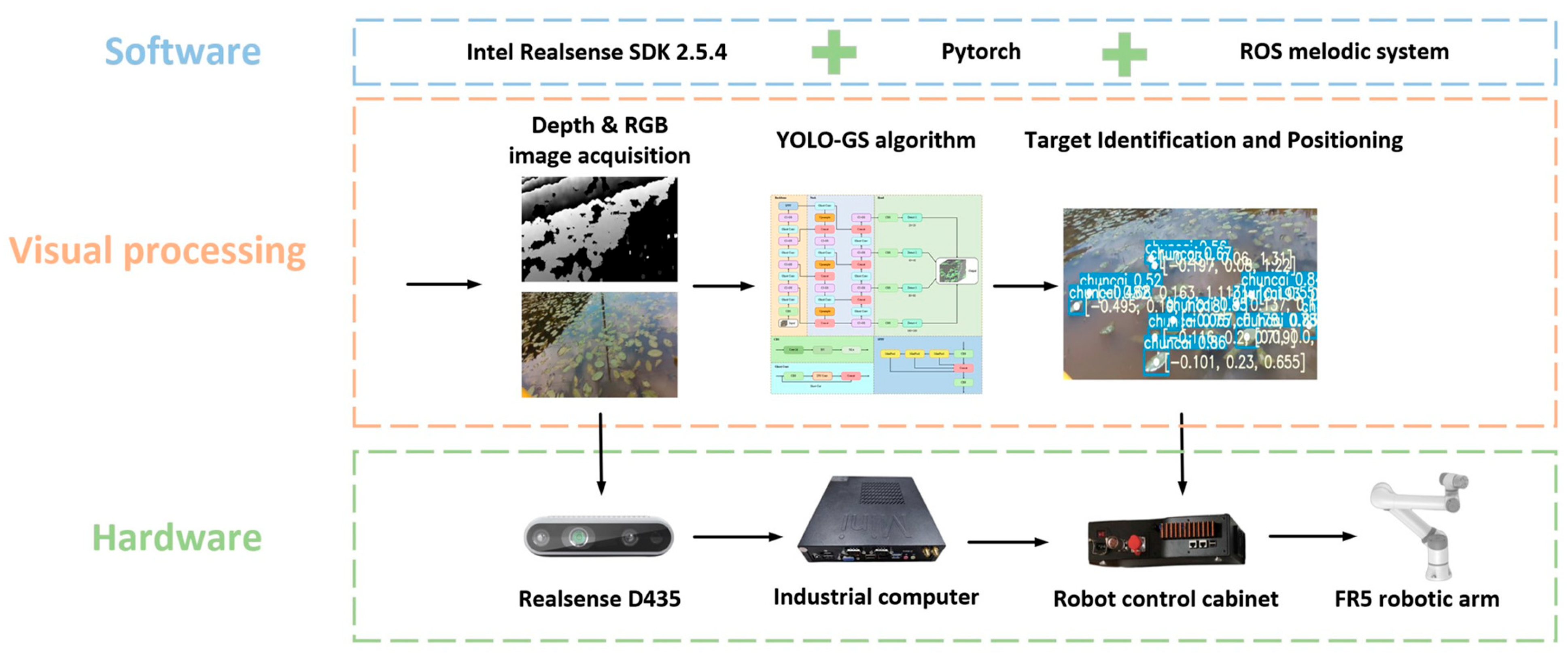
According to the above requirements, we designed a framework, as shown in Figure 2, which is mainly composed of three parts:

• Software part: The software used is based on Ubuntu 18.04 system (Canonical Group Ltd., London, UK), covering the depth camera software Intel Realsense SDK (Intel Corp, Santa Clara, CA, USA), ROS system (Open Robotics, Mountain View, CA, USA), and the YOLO-GS target recognition algorithm based on PyTorch deep learning framework (Facebook, Menlo Park, CA, USA);
• Hardware part: It is mainly composed of D435 depth camera (Intel Corp, Santa Clara, CA, USA), industrial computer (TexHoo, Guangzhou, China), FR5 robot controller, and robotic arm (FAIRINO, Suzhou, China);
• Visual processing stage: Initially, the D435 camera is utilized to capture the RGB and depth data of Brasenia schreberi. Subsequently, the data are sent to the YOLO-GS algorithm running on the industrial computer. The YOLO-GS algorithm enhances the feature extraction capability and recognition accuracy of multi-scale Brasenia schreberi targets in complex environments by utilizing the newly developed C3-GS module and detection head structure. This optimization leads to a significant reduction in computational load and parameters, enabling precise identification of Brasenia schreberi targets. Upon completion of target recognition, the RGB and depth feature information is fused to pinpoint the central picking location of Brasenia schreberi. Finally, the picking location data are converted into the 3D coordinates of the manipulator coordinate system through the coordinate transformation matrix. These coordinates are then transmitted to the robot controller within the ROS system, facilitating actual picking.

Compared with existing frameworks, our framework is different in specific modules and performance. The grape recognition framework flowchart developed by Xu et al. [37] in their study utilizes YOLOv4 and attention mechanism SE recognition algorithm at the software level, along with high-performance GPU computing unit at the hardware level. In comparison to our YOLO-GS algorithm, it incurs a higher computational cost and is not suitable for the visual solution requirements outlined in this research. The flower recognition flowchart created by Wang et al. [34] combines YOLOv4 tiny algorithm with GPU computing devices. While this reduces the computational cost, the recognition accuracy falls below 90%, resulting in a poor recognition effect.

2.2.2. Depth Camera-Based Picking Point Localization

A number of studies related to positioning of fruit and vegetable picking were referenced [35,38]; this paper uses an Intel D435 camera for identification and localization of picking points. The camera has an RGB image sensor, two infrared receivers, and an infrared emitter, which can acquire RGB information and depth information simultaneously.

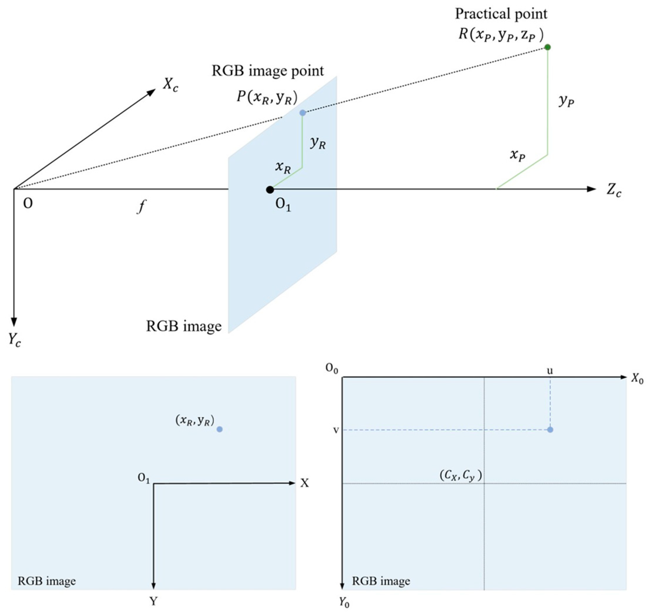
In order to utilize the depth camera for solving the positioning issue of the actual picking point, this study established an imaging model comprising the camera coordinate system, imaging plane, and optical axis based on relevant literature [39]. Subsequently, the transformation relationship of the picking point in the camera coordinate system, image physical coordinate system, and image pixel coordinate system was derived. The positioning principle of the 3D picking point is illustrated in Figure 3. Suppose P is the actual 3D picking point in the scene, and the line from point P to the camera center O intersects with the camera’s imaging plane. The point of intersection is the image point R.

The image physical coordinate system is a 2D rectangular coordinate system. Its origin ${\mathrm{O}}_1$ is the intersection of the $Z_c$-axis of the camera coordinate system and the imaging plane. The $X$-axis is parallel to $X_c$, and the $Y$-axis is parallel to $Y_c$. $\mathrm{O}{\mathrm{O}}_1$ is the focal length $f$ of the camera. Through the similar triangle scale transformation, the transformation relationship between P in the camera coordinate system and R in the image physical coordinate system is obtained, as shown in Equations (1) and (2).

$$x_R=f\frac{X_P}{Z_P}$$

(1)

$$y_R=f\frac{Y_P}{Z_P}$$

(2)

It follows that the generation of practical 3D coordinates needs to be based on depth information $z_P$.

Since pixel information is necessary for aligning the depth map and RGB map, the image pixel coordinate system is established with the upper left corner of the image plane as the origin $O_0$, as depicted in Figure 4. $X_0$ and $Y_0$ are, respectively, parallel to the X-axis and Y-axis of the image physical coordinate system. The coordinates of the origin $O_1$ in the image physical coordinate system are $(c_x,c_y)$ in the pixel coordinate system, and the physical dimensions of each pixel in the X- and Y-axis directions in the image physical coordinate system are $dx$ and $dy$ respectively. Based on the derived Equations (1) and (2), the coordinates of the corresponding point $(u,v)$ of R point in the image pixel coordinate system are presented in Equations (3) and (4):

$$u=\frac{X_R}{dx}+c_x=\frac{f}{dx}\frac{X_P}{Z_P}+c_x=f_x\frac{X_P}{Z_P}+c_x$$

(3)

$$v=\frac{Y_R}{dy}+c_x=\frac{f}{dy}\frac{Y_P}{Z_P}+c_x=f_y\frac{Y_P}{Z_P}+c_y$$

(4)

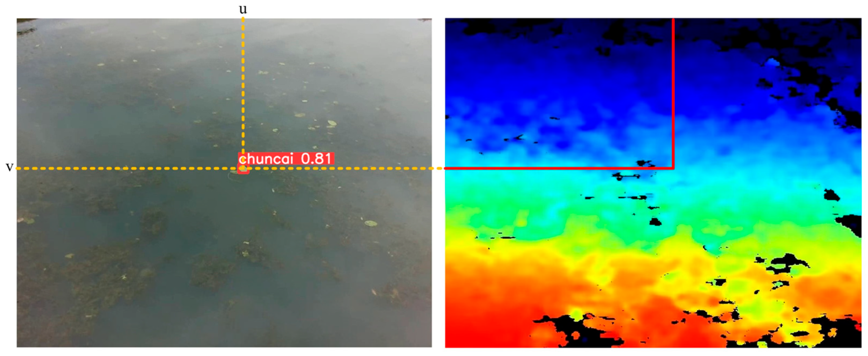
As illustrated in Figure 4, following the previously introduced 3D picking-point positioning principle, the 3D-point coordinates in the camera coordinate system are initially mapped to the imaging plane. Subsequently, the RGB image and depth image are proportionally aligned. The center point of the predicted box in the RGB image corresponds to the coordinate point in the depth image. Ultimately, the depth value of this point is retrieved, allowing for the determination of the depth value $Z_P$ of the actual 3D point.

By transforming Equations (3) and (4), as shown below, on the premise that the value of $Z_P$ is known, the 3D coordinates of the real target point in the camera coordinate system can be obtained.

$$X_P=Z_P\frac{u-c_x}{f_x}$$

(5)

$$Y_P=Z_P\frac{v-c_y}{f_y}$$

(6)

2.3. Data Set Construction

2.3.1. Data Collection and Labelling

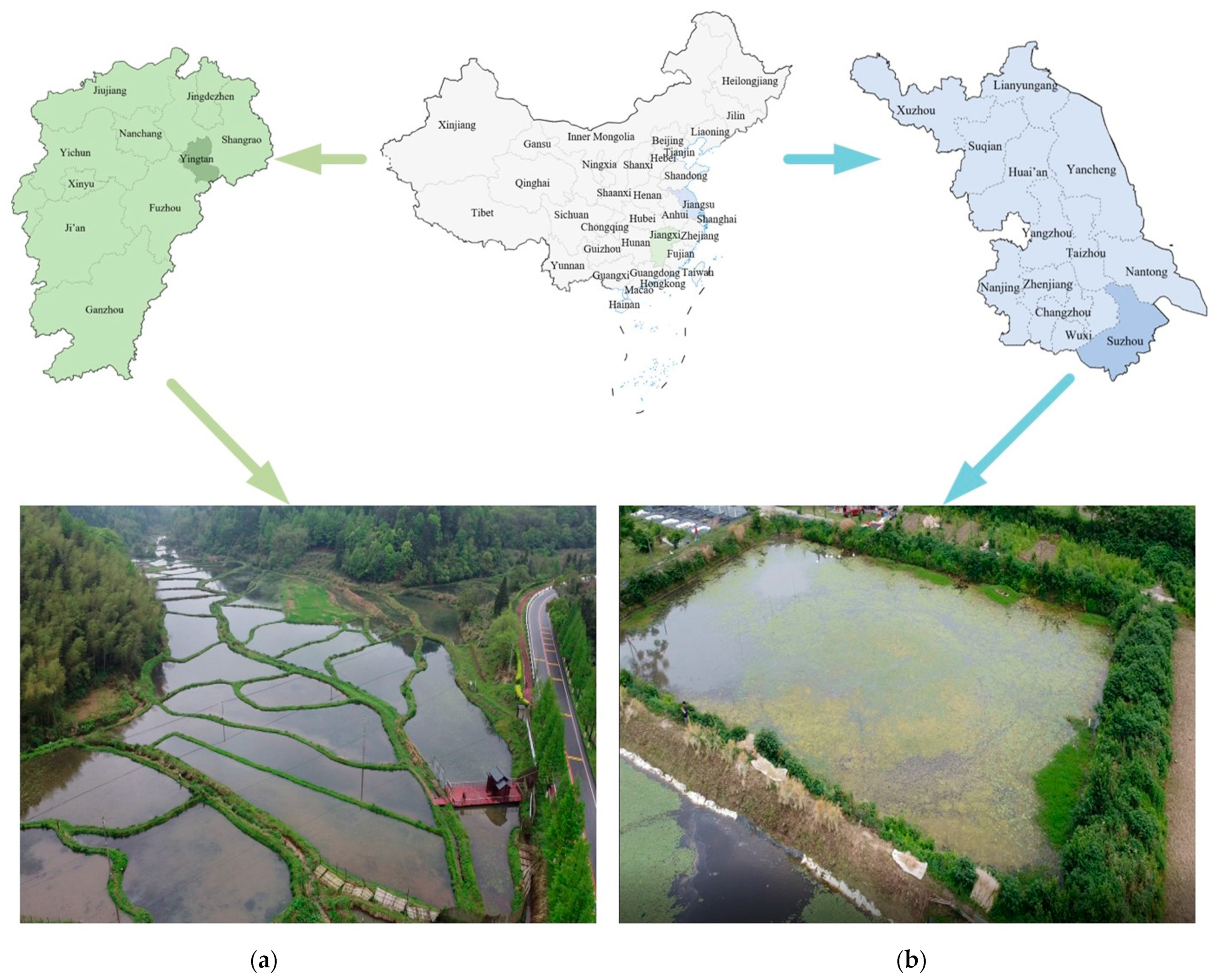
In order to increase the diversity of Brasenia schreberi samples, data sets obtained from two regions were used in this study. One part was collected from the Brasenia schreberi planting base in Yingtan City, Jiangxi Province (coordinates: 117°2′16″ E, 28°4′49″ N), and the other part was collected from the Brasenia schreberi experimental base in Suzhou City, Jiangsu Province (coordinates: 120°43′43″ E, 31°44′22″ N). The image capture time is from 5 June to 31 August 2023, as shown in Figure 5.

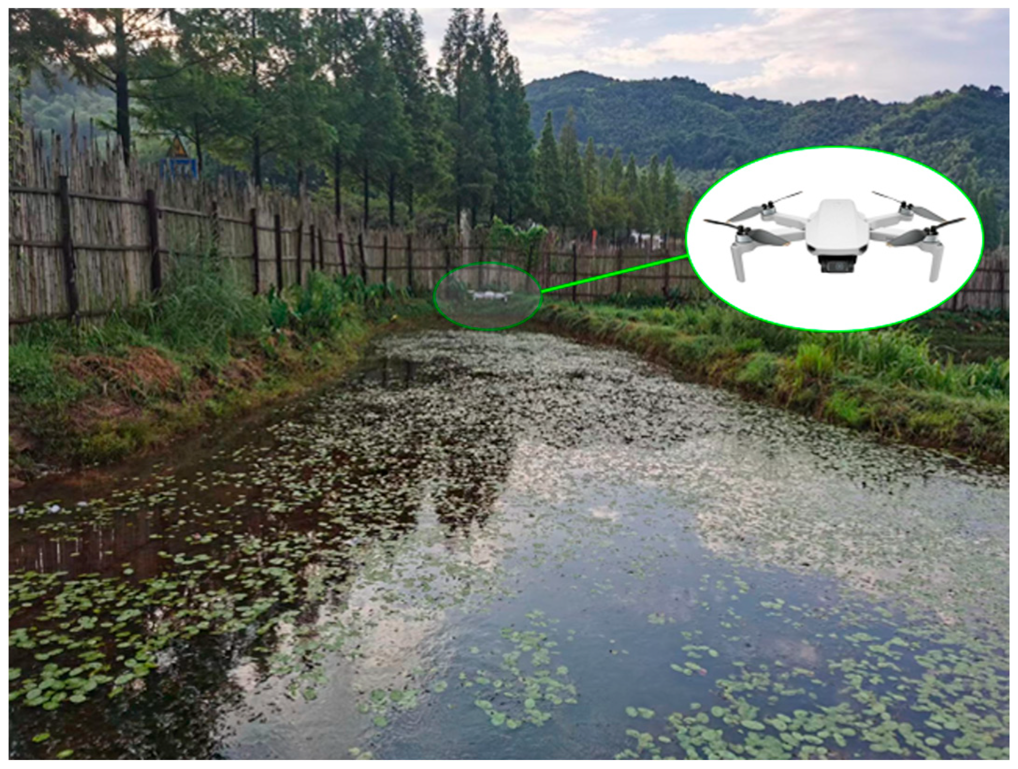
A DJI Mavic mini UAV was used to capture images from 0.5 m to 1 m at pitch angles of 30 to 90 degrees from the horizontal axis, as shown in Figure 6.

One thousand high-quality Brasenia schreberi images with a resolution of 1920 × 1080 were acquired after cropping operations under different lighting conditions, including sunny, cloudy, smooth, and backlighting situations. The original dataset was constituted from them. Labellmg was used to annotate the location information of Brasenia schreberi in the dataset, and the annotated labels were stored in PASCAL VOC format.

2.3.2. Data Enhancement

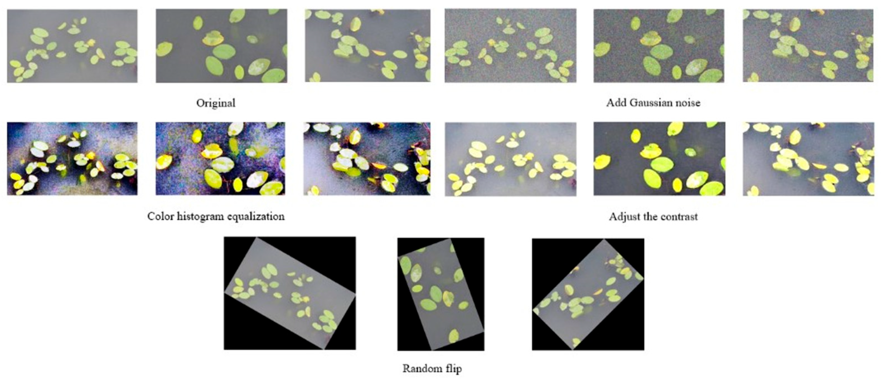
Randomly select the original image data for random flipping, local clipping, length and width scaling, color histogram equalization [40], and median filtering [41], adding Gaussian noise [42], salt and pepper noise, and other operations. According to the previous analysis, the light change factor greatly interferes with target recognition, so the light adaptability of some original data is enhanced by adjusting the contrast and color difference [43]. Increase the data set to 2000 under a series of data enhancement operations. The image enhancement effect is shown in Figure 7. After removing samples with poor image quality through manual screening, the final data set is controlled at 1500 images.

According to the ratio of 7:2:1, the data set is divided into training set, validation set, and test set. The number of images in each data set is 1050, 300, and 150.

2.4. Modelling Improvements

2.4.1. Network Framework for the Improved Algorithm YOLO-GS

With reference to the detection methods in the agricultural domain mentioned in Section 1, we selected YOLOv5 [21] as a template for improvement. The original YOLOv5 consists of three parts: backbone network, neck network, and head network. Its backbone network is responsible for the feature extraction task and mainly consists of the CBS module, the CSP cross-stage bottleneck module, and the SPPF fusion module. The neck uses two network structures, PANET and FPN, to boost the feature fusion capability. The head employs three detection layers with different sizes to predict and fit the target to achieve multi-scale detection and generates a detection frame containing category and confidence information. Depending on the model depth and width, YOLOv5 can be divided into five models from small to large, which are YOLOv5n, YOLOv5s, YOLOv5m, YOLOv5l, and YOLOv5x. Generally speaking, with the increase in network width and depth, the network feature extraction capability will be enhanced, which is intuitively reflected in the AP enhancement. However, parameters, weight size, and computation cost will also increase. In order to deploy on the industrial computer of the harvesting platform with limited computational power, YOLOv5s with smaller model sizes are chosen for improvement.

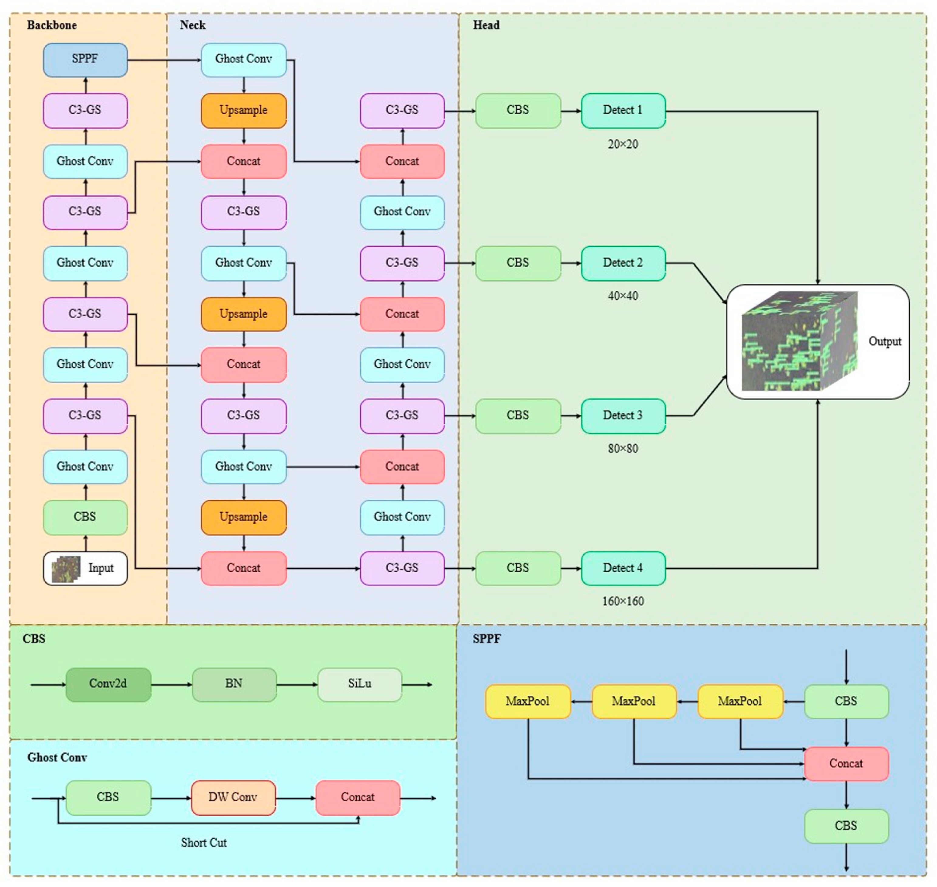
Based on YOLOv5s, a new lightweight network named YOLO-GS was proposed. The architecture of YOLO-GS is shown in Figure 8. The model also consists of three main parts: the backbone, the neck, and the detection head.

Based on the technical difficulties analyzed in the previous section, several improvements were made to the YOLO-GS network compared with the YOLOv5s network. Firstly, to improve the model’s ability to extract and fuse Brasenia schreberi feature information in complex environments, we designed C3-GS, a lightweight CSP module that incorporates a 3D attention mechanism. Secondly, we introduced Ghost Conv [44] to replace the original CBS module to reduce model parameters and computational cost. Additionally, we redesigned the detection head to enhance the recognition effect on multi-scale Brasenia schreberi targets by adding the detection head of 160 × 160, considering the significant size variation of Brasenia schreberi. Finally, Focal EIoU [45] loss function is introduced for better target detection. After recognition, the 2D coordinates of the target are mapped to the depth map to achieve feature fusion of RGB and depth information so as to obtain accurate 3D picking points.

2.4.2. Convolution Module Improvements

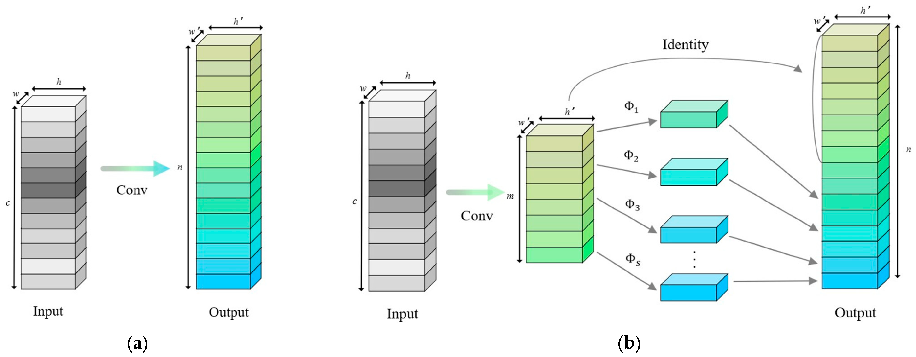
Traditional convolutional neural networks typically consist of numerous convolutions, which entail a significant computational cost. Researchers have been exploring ways to minimize the computational requirements of these models to enable deployment on low-power devices. For example, networks of MobileNet series [46,47] introduce deep separable convolution, reverse residual block, and AutoML technology and are implemented to decrease the computational cost of the model, and ShuffleNet network [48] introduces channel shuffling operation to improve the information flow exchange between channel groups. Their attempt to construct convolutional neural networks using smaller convolutional kernels is undoubtedly fruitful, but the remaining 1 × 1 convolution layers still occupy too much memory and have too many floating-point operations per second (FLOPs). To address this issue, considering the reduction of the characteristic graph of intermediary connections, Ghost module is introduced to try to fundamentally reduce the amount of convolution operation.

The operation of conventional convolution to generate a feature map can be expressed as the following equation:

$$Y=X \ast f+b$$

(7)

$\ast$ is the convolution operation, $b$ is the deviation term, and $\mathrm{Y}\in {\mathbb{R}}^{{\mathrm{h}}^{\prime }\times {\mathrm{w}}^{\prime }\times \mathrm{n}}$ is the output feature map with n channels. $\mathrm{f}\in {\mathbb{R}}^{\mathrm{c}\times \mathrm{k}\times \mathrm{k}\times \mathrm{n}}$ is the convolution kernel for this layer. ${\mathrm{h}}^{\prime }\times {\mathrm{w}}^{\prime }$ is the height of the output data multiplied by the width, and $\mathrm{k}\times \mathrm{k}$ is the kernel size of convolution kernel. The number of floating-point operations per second is $\mathrm{n}\cdot {\mathrm{h}}^{\prime }\cdot {\mathrm{w}}^{\prime }\cdot \mathrm{c}\cdot \mathrm{k}\cdot \mathrm{k}$, which undoubtedly contains many redundant operations. Ghost module removes a part of the approximate feature map generated by the traditional convolution layer and replaces the redundant feature maps with feature maps generated by inexpensive linear operations while keeping the number of feature maps $\mathrm{n}$ in the final output unchanged. The improved equation is as follows:

$${\mathrm{Y}}^{\prime }=\mathrm{X} \ast {\mathrm{f}}^{\prime }$$

(8)

${\mathrm{f}}^{\prime }\in {\mathbb{R}}^{\mathrm{c}\times \mathrm{k}\times \mathrm{k}\times \mathrm{m}}$ is the convolution kernel for the first conventional convolution, and ${\mathrm{Y}}^{\prime }\in {\mathbb{R}}^{{\mathrm{h}}^{\prime }\times {\mathrm{w}}^{\prime }\times \mathrm{m}}$ is the original feature map generated by the first convolution.

$${\mathrm{Y}}_{\mathrm{i}\mathrm{j}}{=\mathrm{\Phi }}_{\mathrm{i}\mathrm{j}}\left({\mathrm{y}}_{\mathrm{i}}^{\prime }\right)\hspace{1em}\hspace{1em}\hspace{1em}\forall i=1,\dots ,m,j=1,\dots ,s$$

(9)

${\mathrm{y}}_{\mathrm{i}}^{\prime }$ is the $i$th original characteristic diagram of ${\mathrm{Y}}^{\prime }$; ${\mathrm{\Phi }}_{\mathrm{i}\mathrm{j}}$ is the $j$th linear operation.

A comparison of the structure of ordinary convolution and Ghost convolution is shown in Figure 9. After theoretical calculations and experimental statistics, Ghost convolution consumes much less computation than ordinary convolution to generate the same number of feature maps.

2.4.3. C3-GS: A Lightweight Cross-Stage Module

In this paper, a new lightweight cross-stage module, C3-GS, is designed. This module can replace the original C3 module in the backbone and neck parts.

simAM [49] is an attention mechanism with parameter number 0. Compared to the common channel attention mechanism or spatial attention mechanism, it is not limited to a single dimension but draws on ideas from the field of neuroscience to consider both the spatial dimension and the channel dimension and assigns a larger weight value to feature maps with higher specificity.

In neuroscience, neurons whose firing patterns are clearly distinct from the rest of the neurons contain richer information and thus deserve to be given higher priority. The simAM attention mechanism defines a neuronal minimum energy function, as shown in Equation (10).

$$e_i^{*}=\frac{4\left({\widehat{\sigma }}^2+\lambda \right)}{(t_i-\widehat{\mu }{)}^2+2{\widehat{\sigma }}^2+2\lambda }$$

(10)

$\lambda$ is the regular term, $i$ is the neuron index, $t_i$ is the value of the $i$th neuron of the input characteristic graph on a single channel, $\widehat{\mu }$ is the mean value of all neurons on a single channel, and ${\widehat{\sigma }}^2$ is the variance of all neurons on a single channel.

The lower the value of $e_i^{*}$, the more difference between the target neuron and the surrounding neurons, indicating that this neuron has a higher level of importance. The weight of a single neuron in the characteristic graph can be represented by $\frac{1}{e_i^{*}}$. $E$ is used to represent the set of $e_i^{*}$ values of all channels and spatial neurons in the feature map and Sigmoid activation function is introduced to limit the excessive value in $E$. The final feature output is shown in Equation (11).

$$\tilde{\mathbf{X}}=sigmoid\left(\frac{1}{\mathbf{E}}\right)\odot \mathbf{X}$$

(11)

$\odot$ is the exclusive nor operator, $\mathbf{X}$ is the input characteristic graph, and $\tilde{\mathbf{X}}$ is the output characteristic graph.

The overall structure of simAM is shown in Figure 10. The input feature map is first weighted by the simAM attention mechanism and then normalized by the sigmoid function. The resulting weight is multiplied by the original feature map element by element and, finally, output.

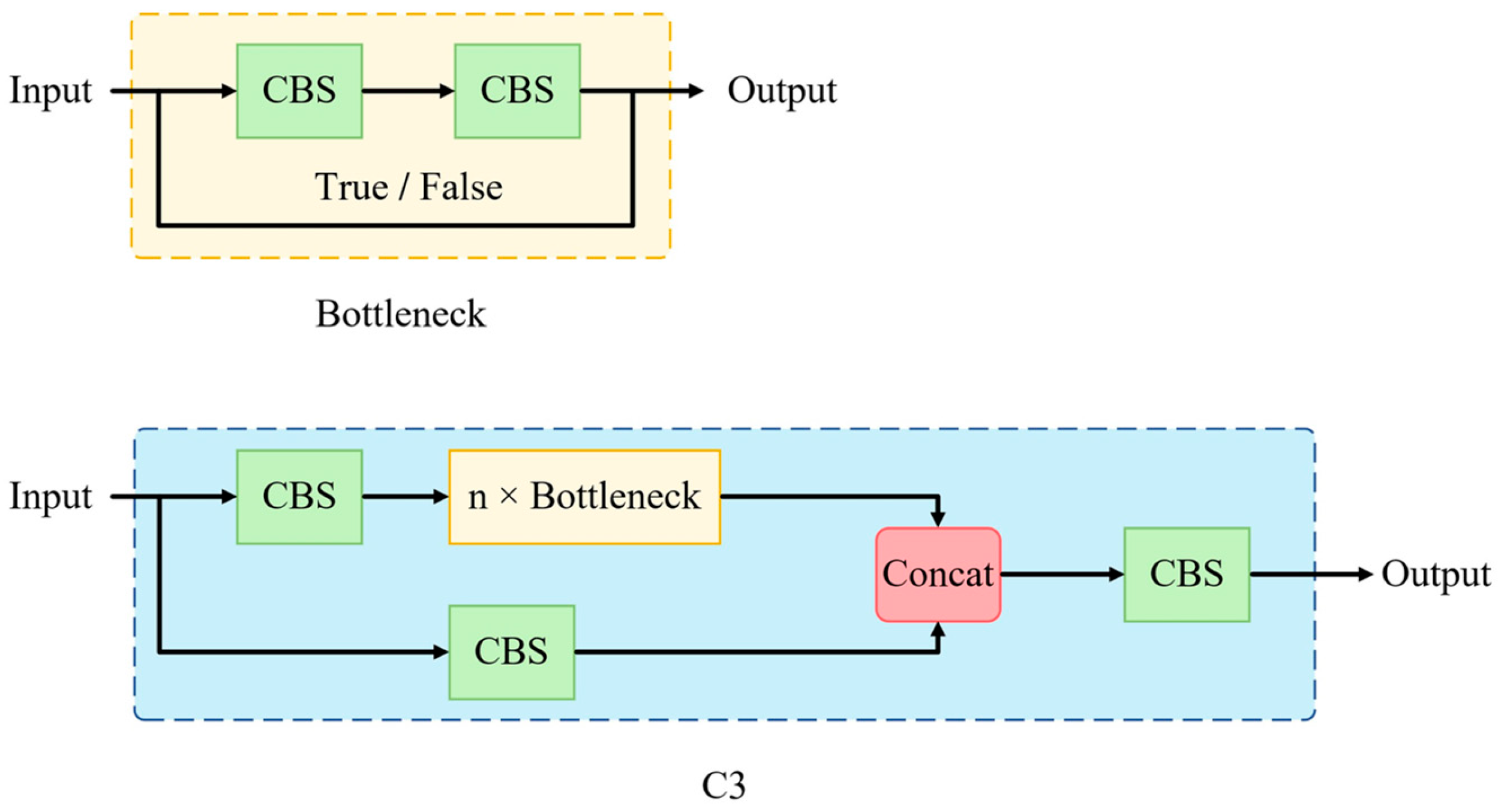
The original C3 structure is depicted in Figure 11 and comprises two branches. One branch traverses a CBS layer and n stacked bottleneck layers. The bottleneck module determines whether to use the residual structure according to the incoming parameters. The other branch solely goes through a CBS layer. Subsequently, the two branches are merged and pass through another CBS layer to yield the final output.

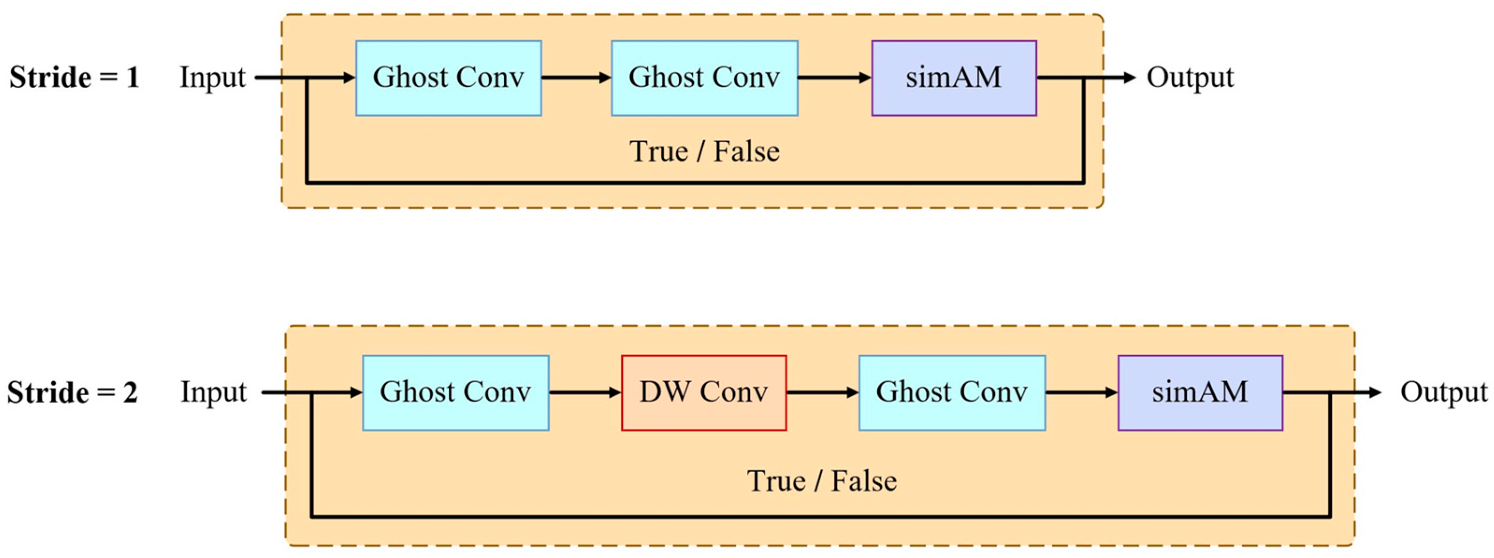
For the purpose of reducing the number of parameters, we use the Ghost bottleneck structure for reference. Considering that the original Ghost bottleneck adopted the network structure of DW convolution and Ghost Conv in series, although it can effectively reduce the number of parameters and calculation, the feature extraction ability is not outstanding, so we chose to embed the simAM attention mechanism in its main path to enhance its ability to learn important features. The improved bottleneck structure is shown in Figure 12.

Apply the newly designed bottleneck structure to improve the C3 structure, as shown in Figure 13. After the experiment, the modification of this network structure effectively improved the recognition accuracy while the number of parameters and the computation amount did not increase.

2.4.4. Detection Head Improvements

In the actual unmanned harvesting process, the Brasenia schreberi in the depth camera view shows a dense distribution of characteristics, while there are obvious size differences due to the fact that the Brasenia schreberi is not exactly in the same growth period.

To mitigate the impact of Brasenia schreberi’s size difference on recognition, enhance the network’s adaptability to various leaf sizes, and boost recognition accuracy in densely populated scenes, this study introduces a small target detection head to the existing three detection heads of the network.

In the neck section, the original 80 × 80 feature map is transformed to 160 × 160 after the up-sampling operation, and the concat operation is performed together with the 160 × 160 feature map in the second layer of the backbone network to generate a new 160 × 160 detection header for detecting the targets with the size of 4 × 4 or more.

The new detection head fuses the shallow feature information in the backbone network and the deep feature information in the neck network, which expands the global sensory field of the model to a certain extent and makes up for the loss of feature information due to continuous down sampling. This improves the recognition effect of the model for Brasenia schreberi at different scales.

2.4.5. Loss Function

Neural networks typically use a loss function to minimize the network error. YOLOv5 uses CIoU [50] to calculate the regression loss using the equation shown below.

$$L_{CIoU}=1-IoU+\frac{{\rho }^2\left(b,b^{gt}\right)}{c^2}+\alpha \upsilon$$

(12)

$b$ is the center point of the prediction box, $b^{gt}$ is the center point of the target box, $\rho \left(·\right)$ is the Euclidean distance, $c$ is the diagonal length of the smallest enclosing box covering the two boxes, $\alpha$ is a positive trade-off parameter, $\upsilon$ is the consistency of aspect ratio, and $IoU$ is the result of dividing the overlap of two regions by the set of two regions.

Taking into account factors such as overlapping area, center-point distance, and aspect ratio in bounding box regression, CIoU has achieved significant improvements in convergence speed and detection accuracy. Although this method has made significant progress in optimizing models compared to traditional loss functions, the aspect ratio factors it covers (represented by the parameter $\upsilon$) sometimes have a negative impact on model optimization.

Therefore, this paper uses the Focal EIoU [45] to calculate the classification loss as shown in Equations (13) and (14):

$${\mathcal{L}}_{EIoU}={\mathcal{L}}_{IoU}+{\mathcal{L}}_{dis}+{\mathcal{L}}_{asp}=1-IoU+\frac{{\rho }^2\left(\mathrm{b},{\mathrm{b}}^{gt}\right)}{c^2}+\frac{{\rho }^2\left(w,w^{gt}\right)}{C_w^2}+\frac{{\rho }^2\left(h,h^{gt}\right)}{C_h^2}$$

(13)

$${\mathcal{L}}_{Focal EIoU}={\mathrm{I}\mathrm{o}\mathrm{U}}^{\gamma }{\mathcal{L}}_{EIoU}$$

(14)

${\mathcal{L}}_{IoU}$ is intersection of union loss, ${\mathcal{L}}_{dis}$ is distance loss, and ${\mathcal{L}}_{asp}$ is orientation loss.

$w$ is the width of the prediction box, $w^{gt}$ is the width of the target box, $h$ is the width of the prediction box, and $h^{gt}$ is the width of the target box.

$C_w$ and $C_h$ are the width and height of the minimum outer bounding box of the two rectangles, respectively, and $\gamma$ is a hyperparameter used to control the degree of outlier suppression.

The Focal EIoU method introduces width height loss on the basis of CIoU, which accelerates convergence speed by minimizing the difference in width and height between the target box and anchor box. At the same time, the Focal Loss strategy is adopted to optimize the sample imbalance problem, reducing the impact of low-quality samples on gradients and making the regression process more focused on high-quality anchor boxes, thereby improving recognition accuracy.

2.5. Model Training

2.5.1. Training Environment and Model Configuration

In the process of model training, the versions of hardware equipment and software architecture have some influence on the training efficiency of the model, so the specific hardware models and software versions are listed in

Table 1. Model training environment.

Environment	Details
GPU	Nvidia GeForce RTX2080ti × 2 (Nvidia Corp, Santa Clara, CA, USA)
CPU	Intel Xeon Silver E5-4216 (Intel Corp, Santa Clara, CA, USA)
Operating system	Windows server 2012r (Microsoft Corp, Redmond, WA, USA)
Python	3.7.13
CUDA	10.1
Pytorch	1.7.0

for reference. In addition, the selection of hyperparameters also affects the performance and generalization ability of the model to a certain extent, so key hyperparameters, such as the number of iterations, batch size, and learning rate, are given in

Table 2. Model training hyperparameters.

Hyperparameters	Details
Epochs	600
Image Size	640 × 640
Batch size	16
Optimizer	SGD
Momentum	0.937
Initial learning rate	0.01

.

2.5.2. Evaluation Indicators

The evaluation metrics in this study include precision (P), recall (R), [email protected], F1 score (F1-Score), model size, parameters, computation, and frames per second (FPS), which are used to evaluate the overall performance of the model in a comprehensive manner, as shown in the following formulas:

$$Precision=\frac{T_P}{T_P+F_P}$$

(15)

$$Recall=\frac{T_P}{T_P+F_N}$$

(16)

$$AP={\int }_0^{1}P\left(R\right)\mathrm{d}R$$

(17)

$$F_1=\frac{2\times Precision\times Recall}{Precision+Recall}$$

(18)

$T_P$ is the true positive example; $F_P$ is the false positive example; $F_N$ is the false negative example.

$F_1$ score is a comprehensive evaluation index combining accuracy and recall.

The precision–recall curve, denoted as P(R), serves as a graphical illustration of the trade-off between precision (vertical axis) and recall (horizontal axis) for varying thresholds within a binary classification model.

3. Results and Discussion

3.1. Visualization of Feature Maps

During the process of image input to the model, the convolutional neural network extracts the features of the image through a series of convolution operations, and the obtained feature map corresponds with the input image. The visual feature map enables us to see the output of the model at different levels more intuitively so that we can understand the basic features learned by each network layer, and it can also play a role as a reference for the evaluation of the recognition effect of the model.

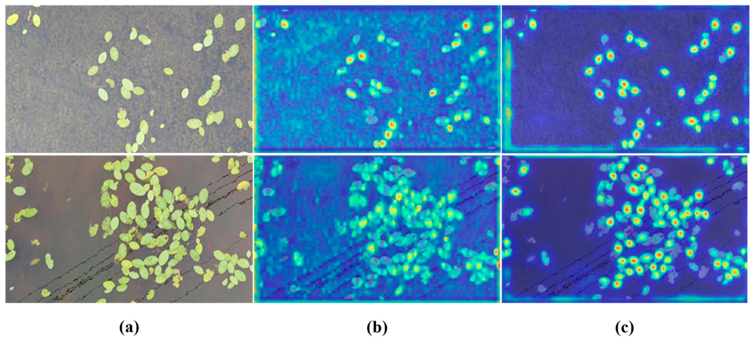
Figure 14 illustrates the results obtained by the Grad-CAM [51]. We selected the concat layer in front of the detected heads for visualization. Our YOLO-GS model has four detection heads in total, so we extracted the feature information of the four layers, 20, 23, 26, and 29, for fusion visualization. The original YOLOv5s model has a total of three detection heads. According to the network structure, the feature information of 16, 19, and 22 layers is extracted for visual processing. As can be seen from Figure 14c, the four-detection-head YOLO-GS model has a significant advantage in contour capture for small-sized leaves. Meanwhile, thanks to the inclusion of the simAM attention mechanism in C3-GS, the focus of recognition is more concentrated, reflecting the model’s improvement in feature extraction capability.

3.2. Comparison of YOLOv5s and YOLO-GS Detection Results

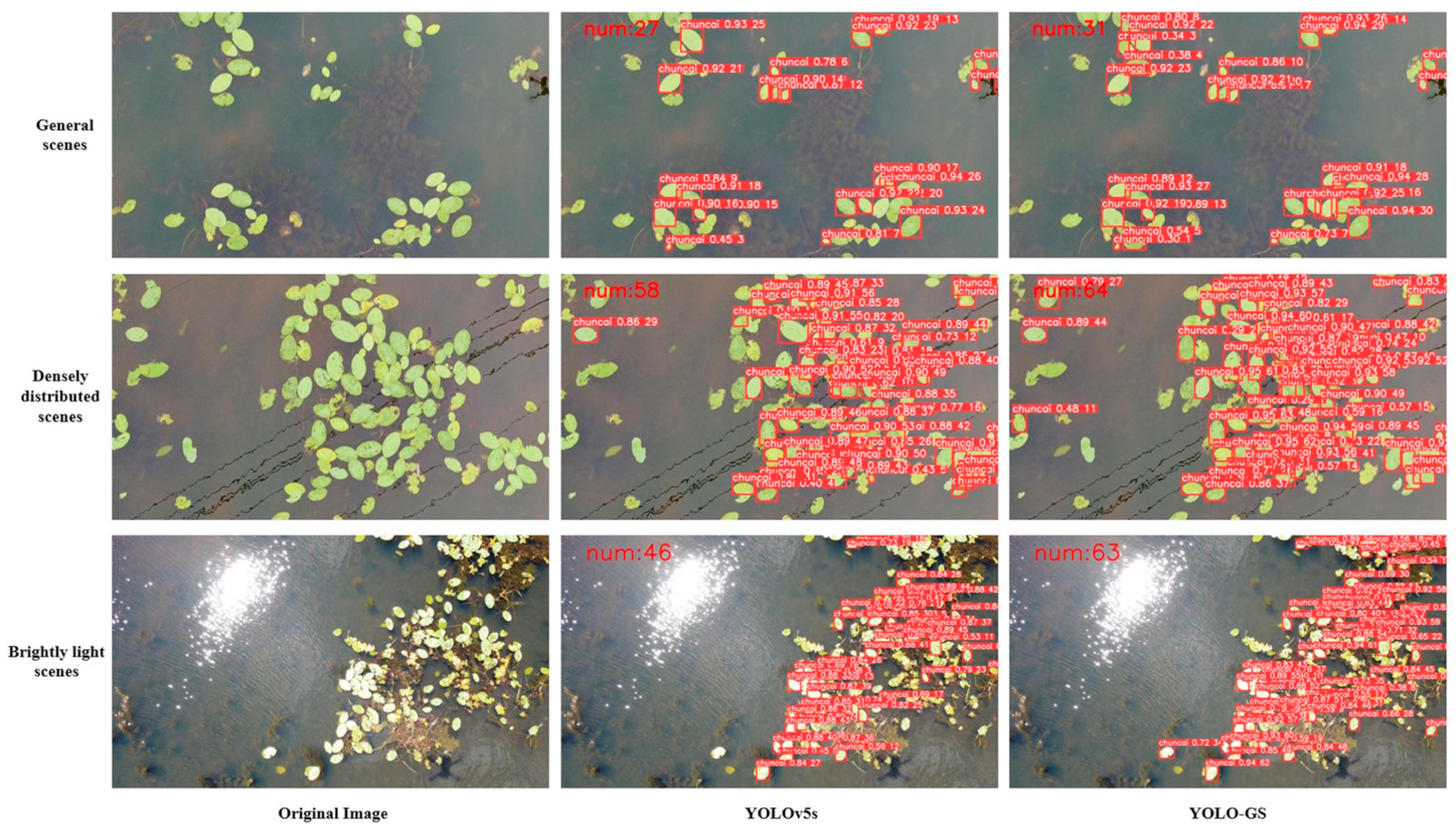
Figure 15 shows the comparison of recognition results between YOLOv5s and YOLO-GS in three cases: a brightly lit scene, a densely distributed scene, and a general scene. It can be seen that the confidence scores of YOLO-GS are generally higher than those of YOLOv5s.

In order to compare the recognition effect of the two more intuitively, a counting function is added to the model to count the number of recognitions. The statistical results are shown in the

Table 3. Comparison of identification results.

Scene	Model	True Quantity	Correctly Identified		Missed
			Amount	Rate (%)	Amount	Rate (%)
General scenes	YOLOv5s	32	27	84.4	5	15.6
	YOLO-GS		31	96.9	1	3.1
Densely distributed scenes	YOLOv5s	66	58	87.9	8	12.1
	YOLO-GS		64	97.0	2	3.0
Brightly lit scenes	YOLOv5s	67	46	68.7	21	31.3
	YOLO-GS		63	94.0	4	6.0

.

In the general scene, the actual number of Brasenia schreberi is 32, YOLOv5s identifies 27, and the leakage rate reaches 15.6%, while YOLO-GS identifies 31, and the leakage rate is only 3.1%. In the densely distributed scene, the actual number of Brasenia schreberi is 66, YOLOv5s identifies 58, and the leakage rate reaches 12.1%, while YOLO-GS identifies 64, and the leakage rate is 3.0%. In the brightly lit scene, the number of actual Brasenia schreberi leaves is 67; YOLOv5s identifies 46, with a leakage rate of 31.3%, while YOLO-GS identifies 63, with a leakage rate of 6.0%. YOLOv5s presents a higher leakage rate in all three scenarios, with much higher leakage rates in the case of bright light. In contrast, YOLO-GS has little leakage detection and not only has a good recognition effect on overlapping occlusion targets in densely distributed scenes but is also basically not affected by water reflections, which verifies that YOLO-GS improves the feature extraction capability in complex environments while enhancing the light adaptation of the algorithm.

3.3. Ablation Experiments

In order to visualize the effects of the Ghost Conv module, C3-GS module, four-head improvement, and Focal EIoU loss function on the model performance, this study conducts ablation experiments using the previously mentioned dataset and a unified training environment as a means of verifying the improvement of the model performance.

As shown in

Table 4. Ablation experiment results.

Model	Ghost Conv	C3-GS	4-Head	Precision	Recall	F1-Score	[email protected]	Weight Size (MB)	GFLOPS
YOLOv5s	×	×	×	89.9	87.5	88.7	92.9	14.1	15.8
Model 1	√	×	×	88.5	90.2	89.3	94.7	11.3	13.4
Model 2	×	√	×	88.9	90.6	89.7	94.1	9.69	10.4
Model 3	×	×	√	88.9	90.4	89.6	94.9	14.3	18.5
Model 4	√	√	×	89.0	90.0	89.5	94.9	7.39	8.0
Model 5	×	√	√	89.1	91.1	90.1	95.7	10.2	12.2
Model 6	√	×	√	88.9	90.8	89.8	95.5	12.0	15.9
Model 7	√	√	√	89.2	90.3	89.7	95.6	7.95	9.5

, compared with the benchmark model YOLOv5s, the Ghost Conv improvement is able to increase the mAP while reducing the number of parameters and computations. Despite the decrease in precision, all other metrics have been improved, which can meet the lightweight requirements of unmanned harvesting tasks. The newly designed C3-GS module achieves a 1.2% increase in mAP due to the addition of the simAM attention mechanism. At the same time, the convolution in the bottleneck structure is also replaced by Ghost Conv, and the number of parameters and calculations is significantly reduced. Due to the increase in the number of network layers, the four-head improvement inevitably increases the amount of calculation and parameters of the model but brings a 2% increase in mAP. Comparing the model 7 resulting from the combination of these three improvements with YOLOv5s, the F1-Score is improved by 1%, the mAP is improved by 2.7%, the model size is reduced by 43.6%, and the computation is reduced by 39.9%.

After ablation experiments, the current optimal model, Model 7, is derived. At this time, the regression loss function used is the CIoU of the original YOLOv5s. In order to verify the effect of the Focal EIoU loss function on the improvement of the model, we introduce SIoU [52], NWD [53], EIoU [45], alpha IoU [54] loss functions for training and testing. Compared with the original CIoU, these IoU algorithms do not have significant differences in GFLOPs and model sizes, and there are slight differences in detection accuracy. The results are shown in

Table 5. Comparison of loss functions.

Model	Precision	Recall	F1-Score	[email protected]
Model 7-CIoU	89.2	90.3	89.7	95.6
Model 7-EIoU	88.5	91.1	89.8	95.5
Model 7-NWD	90.6	87.5	89.0	95.3
Model 7-alphaIoU	87.0	92.2	89.5	95.4
Model 7-SIoU	88.9	90.2	89.5	95.4
Model 7-Focal EIoU	89.1	89.5	89.3	95.7

.

Experiments show that the improved model with the Focal EIoU loss function has the best mAP of 95.7%; therefore, the Focal EIoU loss function is the most effective in improving the model performance in the training test of the loss function.

Figure 16 shows the loss function curve of the original YOLOv5s and YOLO-GS in the training process. It can be seen that at the beginning of the training, the gradient of the loss function decreases rapidly. When the iteration rounds reach 200, the gradient of the loss function continues to decline, but the trend gradually slows down. Until 600 rounds of iteration are completed, the curve has tended to be stable, and the loss function converges to a fixed value, ending the training. During this process, the loss function did not show overfitting. Compared with the original YOLOv5s, YOLO-GS with the Focal EIoU loss function has a faster overall convergence speed, lower training loss values, and smaller fluctuations in the loss values. The final box loss, object loss, and total loss of YOLOv5s are 0.019, 0.048, and 0.067, respectively, while the final loss values of YOLO-GS are 0.017, 0.025, and 0.042, respectively, which are reduced to a certain extent compared with YOLOv5s, verifying that the predictive ability of the model is enhanced.

3.4. Performance Comparison of Different Models

In order to further test and improve the performance of the model, this section selects Faster RCNN [20], SSD [26], YOLOv3 [24], YOLOv3-tiny [55], YOLOv4 [25] YOLOv4-tiny [56], YOLOv5s, YOLOv6s [22], and YOLOv7s [23] as the comparison objects. The detection performance of the YOLO-GS model is compared with other common advanced detection models trained on the Brasenia schreberi dataset. In order to respond to the comprehensive index of each model as objectively as possible, precision (P), recall (R), [email protected], and F1 score (F1-Score) are selected as the evaluation indexes for recognition accuracy. Due to the need to deploy on the industrial control computer with only a CPU and CPU detection speed, FPS is selected as the evaluation index of model performance. In addition, the weight size, parameters, and GFLOPS are compared to make an evaluation from the perspective of both accuracy and performance. The results of the comparative assessment are shown in

Table 6. Comparison of common advanced detection models.

Models	Precision/%	Recall/%	F1/%	[email protected]	Parameters (M)	Weight Size (MB)	GFLOPS	Detect Speed (FPS)
YOLOv5s	89.9	87.5	88.7	92.9	7.01	14.1	15.8	24.9
YOLOv6s	80.7	87.1	83.8	95.0	18.5	38.7	45.2	23.1
YOLOv7	89.0	91.6	90.3	95.8	36.5	71.3	103.2	6.6
YOLOv4	89.9	82.9	86.3	94.8	63.9	245	141.9	3.7
YOLOv4-tiny	87.5	82.5	84.9	91.7	5.9	23	16.2	20.4
YOLOv3	89.4	84.8	87.0	92.5	61.5	117	154.5	5.8
YOLOv3-tiny	88.9	85.7	87.3	90.1	8.7	36.6	12.9	25.3
SSD	84.7	81.9	83.3	91.0	23.6	90.6	136.6	4.5
Faster-RCNN	63.5	90.9	74.8	83.8	136.7	521.0	200.8	0.8
YOLO-GS	89.1	89.5	89.3	95.7	3.75	7.95	9.5	28.7

.

The 10 models mentioned above can be categorized into one two-stage model, Faster-RCNN, and the remaining nine single-stage models based on their implementation steps. Analysis of the experimental data in Table 6 reveals that despite the incorporation of a regional proposal network to aid in generating candidate regions and achieving faster detection speed, Faster RCNN exhibits notably inferior performance in Brasenia schreberi identification compared to the other single-stage models. This is attributed to its inherent characteristic of first generating candidate boxes before classifying and localizing, resulting in a detection speed of only 0.8 $f·s^{-1}$ during recognition tasks, which is merely 2.8% of YOLO-GS’s capability and renders it unsuitable for autonomous vegetable harvesting tasks. Among the single-stage models, SSD stands out due to its utilization of a shallow VGG as its main network, leading to weaker feature extraction capabilities compared to the YOLO series models. Despite having more parameters and higher computational complexity, SSD also demonstrates lower recognition accuracy than YOLO-GS by 4.7%. Subsequently, we will delve into an examination of the YOLO series models. The models represented by YOLOv3, YOLOv4, and YOLOv7 possess numerous parameters and high computational complexity, leading to significant computation costs. While they achieve commendable detection accuracy, their real-time performance is subpar. On the other hand, YOLOv3-tiny and YOLOv4-tiny achieve satisfactory real-time performance through simplification of network layers from their original counterparts. However, their detection accuracy also decreased by 5.6% and 4.0% compared to YOLO-GS, respectively.

Analyzing the important indicators, in terms of [email protected] and F1 score, YOLO-GS reaches 95.7% and 89.3%, respectively, which is better than most of the networks and is only 0.1% and 1% lower than YOLOv7. However, the model size and the number of parameters of YOLO-GS are only 11.2% and 10.3% of YOLOv7, and the detection speed is even faster than YOLOv7 by 342.4%. Compared with YOLOv7, thanks to the improved C3-GS module, YOLO-GS has significant advantages in terms of computation cost and real-time performance, which is more suitable for the technical requirements of unmanned harvesting. In the compared networks, YOLO-GS has the fastest CPU detection speed of 28.7 $f·s^{-1}$ and 15.3% faster than the benchmark model YOLOv5s. Compared with YOLOv3-tiny, YOLOv4-tiny, and YOLOv6s, which are also lightweight networks, it is 13.4%, 40.7%, and 19.5% faster, respectively. It reflects the remarkable results of the proposed method in real time. It is worth noting that YOLO-GS also has the lowest number of parameters and computation amount among all the compared networks as well, with the number of parameters reduced to an astonishing 3.75 M and the computation amount reduced to 9.5 GFLOPS, which reflects its outstanding advantage in terms of computation cost, which allows our method to have lower hardware requirements to better adapt to the industrial computers with weak performance.

3.5. Picking Point Localisation Experiments Combined with Depth Camera

In order to verify the positioning accuracy of this research method, the picking-point positioning experiment was designed. The picking-point positioning experiment included the following steps:

• Activate the RealSense D435 camera to continuously acquire RGB and depth image information;
• The RGB image information is passed to the YOLO-GS algorithm deployed on the industrial controller for recognition;
• The YOLO-GS algorithm starts interacting with the depth camera in real time, aligning the depth image with the RGB image;
• When a harvestable target (distance less than 1.0 m) enters the camera’s field of view, the identification frame is drawn in real time, and the $(u,v)$ coordinates of its center point in the RGB image are obtained;
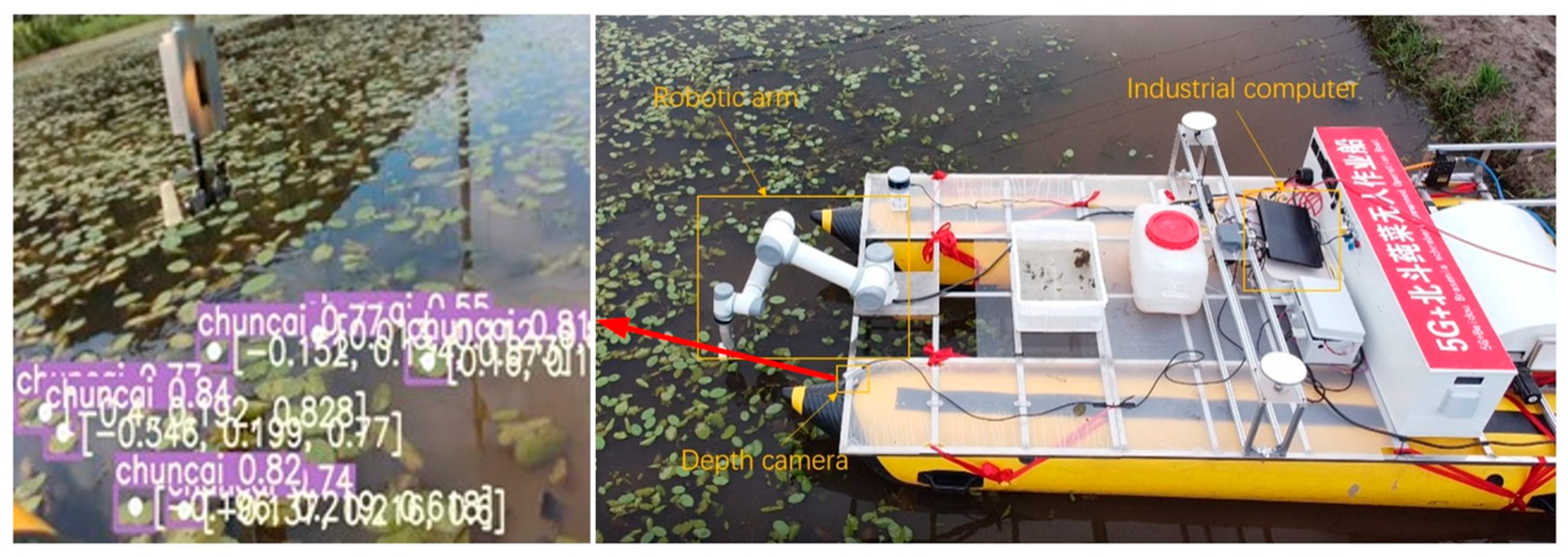
• Map the $(u,v)$ coordinates of the RGB image to the depth image to obtain the corresponding depth coordinate $z_P$, and generate the target-point coordinates $(x_P,y_P,z_P)$ in the camera coordinate system, as shown in Figure 17;
• Calculate the coordinate difference between the target-point coordinates $(x_P,y_P,z_P)$ and the practical picking point, take the absolute value, and finally obtain the error in each direction on the X-axis, Y-axis, and Z-axis.

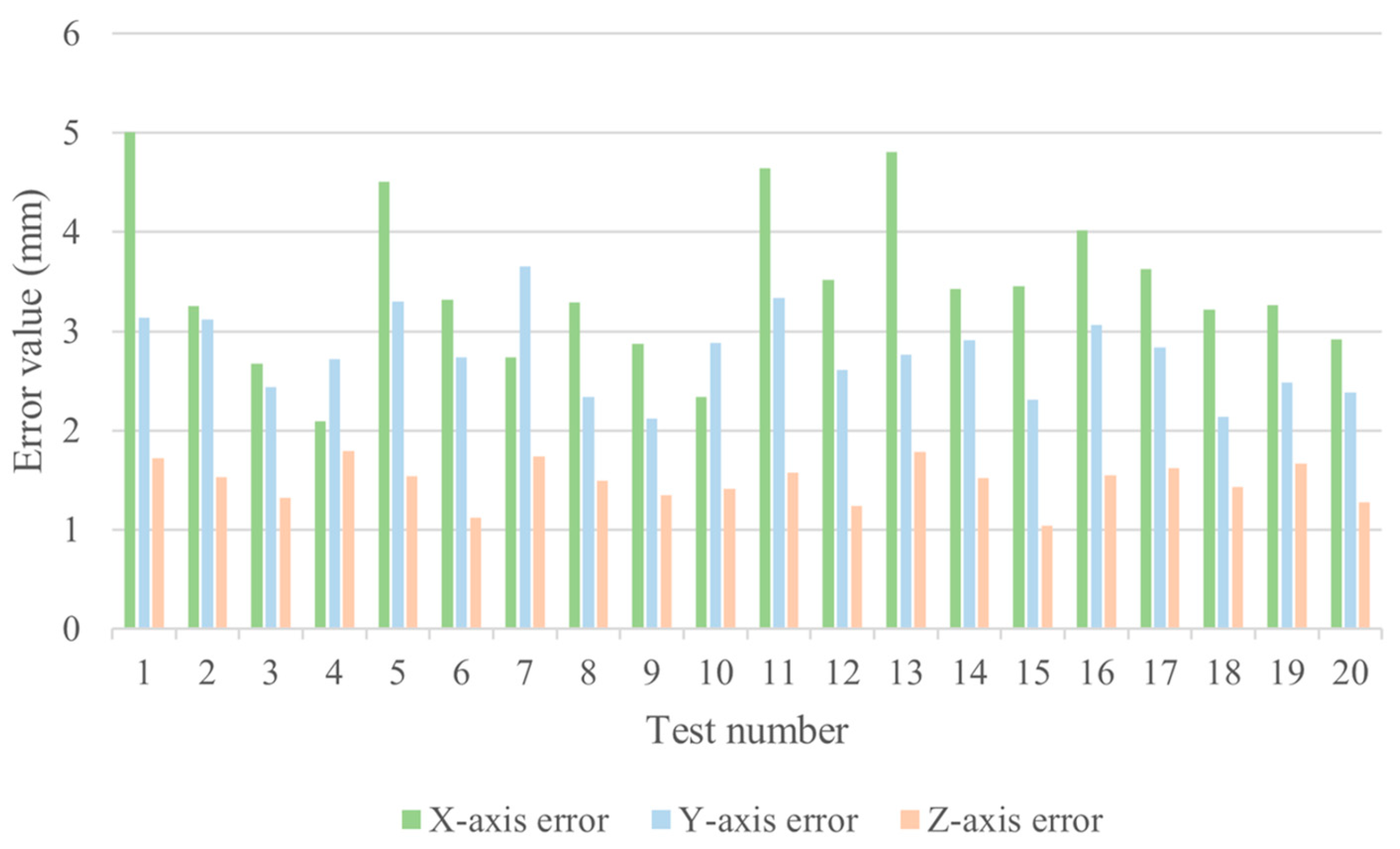
Twenty groups of positioning tests were conducted, and the statistical error data were visually analyzed, as shown in Figure 18.

Under the camera coordinate system, the maximum error between the real picking-point coordinate and the theoretical target-point coordinate in the X-axis direction is 5.01 mm, with an average error of 3.45 mm. The maximum error in the Y-axis direction is 3.65 mm, and the average error is 2.76 mm. The maximum error in the Z-axis is 1.79 mm, and the average error is 1.24 mm. Considering that the allowable error range of the end effector is 25 mm, the positioning error of the picking point is far less than this range. Therefore, the recognition and positioning method combined with the depth camera can meet the demand for unmanned harvesting.

4. Conclusions

In this study, we collected and produced a kind of Brasenia schreberi data set containing 1500 pictures for the task of unmanned picking of aquatic vegetables, which greatly enriched the data samples of Brasenia schreberi, an aquatic vegetable. Based on this data set, we studied a multi-feature fusion lightweight Brasenia schreberi recognition algorithm YOLO-GS.

This study introduces a new approach based on YOLOv5s architectural improvements to optimize the target recognition performance through algorithmic improvements such as the Ghost convolution module, the C3-GS cross-stage attention fusion module, a new detection head structure, and the Focal EIoU loss function.

Through ablation experiments, YOLO-GS reduces parameters by 46.5%, computation by 39.9%, and model size by 43.6%; increases mAP by 2.8%; and boosts FPS by 15.2% compared to YOLOv5s. This enhances recognition accuracy while reducing computation power costs. Comparative experiments of feature map visualization and different scene recognition effects show that YOLO-GS has significantly improved its feature extraction ability and illumination adaptability. When compared with nine advanced detection algorithms, YOLO-GS demonstrates significant advantages in parameters, computation, model size, and CPU detection speed. The mAP is only 0.1% lower than the highest YOLOv7, while the detection speed is faster than YOLOv7 by 342.4%.

The experimental results above demonstrate that the innovation in this study addresses three technical challenges in unmanned aquatic vegetable harvesting tasks: managing computational costs, overcoming light interference, and reducing the occurrence of false detections in complex environments. Building on this foundation, the paper proposes a practical vision system that integrates hardware components like a robotic arm, depth camera, and industrial computer with software frameworks such as the YOLO-GS network model and ROS. This system generates 3D picking points needed for actual harvesting by fusing depth and RGB information features and validates the accuracy of the research method through experiments on picking-point positioning.

Practical unmanned harvesting solutions rely heavily on accurate target identification and localization methods that are both precise and cost-effective. The method proposed in this study demonstrates notable enhancements in identifying and locating targets in complex scenarios through modular optimization and the integration of multi-feature information. It surpasses the most cutting-edge identification algorithms specifically designed for unmanned harvesting of aquatic vegetables. Emphasizing cost efficiency, this method stands out for its significant reduction in parameters and computational workload, making it suitable for deployment on low-power industrial controllers for unmanned harvesting platforms.

This study will focus on the following two aspects in the future:

• Further expand the data set. On the one hand, the Brasenia schreberi are classified according to the growth period, and the distinction between fresh Brasenia schreberi and aging Brasenia schreberi is made so as to achieve more refined picking operations. On the other hand, the roots, leaves, and buds of vegetables are used for different purposes. When picking, classification should be realized according to different picking purposes, and the data sets should be made for different parts of Brasenia schreberi;
• Expand the application. The identification and positioning method proposed in this paper can also be used in the field of crop monitoring and analysis. Combined with the improved counting program, it can monitor the growth status of crops in the designated area in real time and provide information support for fertilization and pesticide application in agricultural production activities;
• On the basis of the target recognition and positioning method we studied, we will analyze the harvesting cost of aquatic vegetables from the perspective of economy and efficiency, compared with manual picking and picking methods based on other algorithm frameworks, and explore the scheme of unmanned harvesting of aquatic vegetables with the best comprehensive cost.

References

1. Peter, K.V. Potential of Aquatic Vegetables in the Asian Diet. In Proceedings of the Seaveg, High Value Vegetables in Southeast Asia: Production, Supply & Demand, Chiang Mai, Thailand, 24–26 January 2012; pp. 210–215. [Google Scholar]
2. Yang, C.; Zhang, X.; Seago, J.L., Jr.; Wang, Q. Anatomical and Histochemical Features of Brasenia schreberi (Cabombaceae) Shoots. Flora 2020, 263, 151524. [Google Scholar] [CrossRef]
3. Liu, G.; Feng, S.; Yan, J.; Luan, D.; Sun, P.; Shao, P. Antidiabetic Potential of Polysaccharides from Brasenia schreberi Regulating Insulin Signaling Pathway and Gut Microbiota in Type 2 Diabetic Mice. Curr. Res. Food Sci. 2022, 5, 1465–1474. [Google Scholar] [CrossRef] [PubMed]
4. Li, J.; Yi, C.; Zhang, C.; Pan, F.; Xie, C.; Zhou, W.; Zhou, C. Effects of Light Quality on Leaf Growth and Photosynthetic Fluorescence of Brasenia schreberi Seedlings. Heliyon 2021, 7, e06082. [Google Scholar] [CrossRef] [PubMed]
5. Yang, Y.; Li, J.; Wang, N.; Zou, X.; Zou, S. The Complete Chloroplast Genome Sequence of Brasenia schreberi (Cabombaceae). Mitochondrial DNA Part B 2019, 4, 3842–3843. [Google Scholar] [CrossRef] [PubMed]
6. Feng, S.; Luan, D.; Ning, K.; Shao, P.; Sun, P. Ultrafiltration Isolation, Hypoglycemic Activity Analysis and Structural Characterization of Polysaccharides from Brasenia schreberi. Int. J. Biol. Macromol. 2019, 135, 141–151. [Google Scholar] [CrossRef] [PubMed]
7. Otsu, N. Threshold Selection Method from Gray-Level Histograms. IEEE Trans. Syst. Man Cybern. 1979, 9, 62–66. [Google Scholar] [CrossRef]
8. Lowe, D.G.; Lowe, D.G. Distinctive Image Features from Scale-Invariant Key-Points. Int. J. Comput. Vis. 2004, 60, 91–110. [Google Scholar] [CrossRef]
9. Dalal, N.; Triggs, B. Histograms of Oriented Gradients for Human Detection. In Proceedings of the IEEE Computer Society Conference on Computer Vision & Pattern Recognition, San Diego, CA, USA, 20–25 June 2005. [Google Scholar]
10. Hartigan, J.A.; Wong, M.A. A K-Means Clustering Algorithm. Appl. Stat. 1979, 28, 100–108. [Google Scholar] [CrossRef]
11. Kanungo, T.; Mount, D.M.; Netanyahu, N.S.; Piatko, C.D.; Silverman, R.; Wu, A.Y. An Efficient K-Means Clustering Algorithm: Analysis and Implementation. IEEE Trans. Pattern Anal. Mach. Intell. 2002, 24, 881–892. [Google Scholar] [CrossRef]
12. Canny, J. A Computational Approach to Edge Detection. IEEE Trans. Pattern Anal. Mach. Intell. 1986, PAMI-8, 679–698. [Google Scholar] [CrossRef]
13. Leavers, V.F. Shape Detection in Computer Vision Using the Hough Transform; Springer: New York, NY, USA, 1992. [Google Scholar]
14. Cortes, C.; Vapnik, V. Support-Vector Networks. Mach. Learn. 1995, 20, 273–297. [Google Scholar] [CrossRef]
15. Benalcázar, M.E. Machine Learning for Computer Vision: A Review of Theory and Algorithms. RISTI—Rev. Iber. De Sist. E Tecnol. Inf. 2019, E19, 608–618. [Google Scholar]
16. LeCun, Y.; Bengio, Y.; Hinton, G. Geoffrey Deep Learning. Nature 2015, 521, 436–444. [Google Scholar] [CrossRef]
17. Attri, I.; Awasthi, L.K.; Sharma, T.P.; Rathee, P. A Review of Deep Learning Techniques Used in Agriculture. Ecol. Inform. 2023, 77, 102217. [Google Scholar] [CrossRef]
18. Li, W.; Zheng, T.; Yang, Z.; Li, M.; Sun, C.; Yang, X. Classification and Detection of Insects from Field Images Using Deep Learning for Smart Pest Management: A Systematic Review. Ecol. Inform. 2021, 66, 101460. [Google Scholar] [CrossRef]
19. Girshick, R. Fast R-CNN. In Proceedings of the 2015 IEEE International Conference on Computer Vision (ICCV), Santiago, Chile, 7–13 December 2015; pp. 1440–1448. [Google Scholar]
20. Ren, S.; He, K.; Girshick, R.; Sun, J. Faster R-CNN: Towards Real-Time Object Detection with Region Proposal Networks. IEEE Trans. Pattern Anal. Mach. Intell. 2017, 39, 1137–1149. [Google Scholar] [CrossRef] [PubMed]
21. Jocher, G. YOLOv5 by Ultralytics; Zenodo: Geneva, Switzerland, 2020. [Google Scholar]
22. Li, C.; Li, L.; Jiang, H.; Weng, K.; Geng, Y.; Li, L.; Ke, Z.; Li, Q.; Cheng, M.; Nie, W.; et al. YOLOv6: A Single-Stage Object Detection Framework for Industrial Applications. arXiv 2022, arXiv:2209.02976. [Google Scholar]
23. Wang, C.-Y.; Bochkovskiy, A.; Liao, H.-Y.M. YOLOv7: Trainable Bag-of-Freebies Sets New State-of-the-Art for Real-Time Object Detectors. In Proceedings of the 2023 IEEE/CVF Conference on Computer Vision and Pattern Recognition (CVPR), Vancouver, BC, Canada, 18–22 June 2023; pp. 7464–7475. [Google Scholar]
24. Redmon, J.; Farhadi, A. Yolov3: An Incremental Improvement. arXiv 2018, arXiv:1804.02767. [Google Scholar]
25. Bochkovskiy, A.; Wang, C.-Y.; Liao, H.-Y.M. Yolov4: Optimal Speed and Accuracy of Object Detection. arXiv 2020, arXiv:2004.10934. [Google Scholar]
26. Liu, W.; Anguelov, D.; Erhan, D.; Szegedy, C.; Reed, S.; Fu, C.-Y.; Berg, A.C. SSD: Single Shot MultiBox Detector. In Proceedings of the Computer Vision—ECCV 2016, Amsterdam, The Netherlands, 11–14 October 2016; Leibe, B., Matas, J., Sebe, N., Welling, M., Eds.; Springer International Publishing: Cham, Switzerland, 2016; pp. 21–37. [Google Scholar]
27. Jin, X.; Jiao, H.; Zhang, C.; Li, M.; Zhao, B.; Liu, G.; Ji, J. Hydroponic Lettuce Defective Leaves Identification Based on Improved YOLOv5s. Front. Plant Sci. 2023, 14, 1242337. [Google Scholar] [CrossRef]
28. Hajam, M.A.; Arif, T.; Khanday, A.M.U.D.; Neshat, M. An Effective Ensemble Convolutional Learning Model with Fine-Tuning for Medicinal Plant Leaf Identification. Information 2023, 14, 618. [Google Scholar] [CrossRef]
29. Yadav, S.; Sengar, N.; Singh, A.; Singh, A.; Dutta, M.K. Identification of Disease Using Deep Learning and Evaluation of Bacteriosis in Peach Leaf. Ecol. Inform. 2021, 61, 101247. [Google Scholar] [CrossRef]
30. Zhang, Z.; Lu, Y.; Yang, M.; Wang, G.; Zhao, Y.; Hu, Y. Optimal Training Strategy for High-Performance Detection Model of Multi-Cultivar Tea Shoots Based on Deep Learning Methods. Sci. Hortic. 2024, 328, 112949. [Google Scholar] [CrossRef]
31. Yang, J.; Chen, Y. Tender Leaf Identification for Early-Spring Green Tea Based on Semi-Supervised Learning and Image Processing. Agronomy 2022, 12, 1958. [Google Scholar] [CrossRef]
32. Chaivivatrakul, S.; Moonrinta, J.; Chaiwiwatrakul, S. Convolutional Neural Networks for Herb Identification: Plain Background and Natural Environment. Int. J. Adv. Sci. Eng. Inf. Technol. 2022, 12, 1244–1252. [Google Scholar] [CrossRef]
33. Zhu, W.; Sun, J.; Wang, S.; Shen, J.; Yang, K.; Zhou, X. Identifying Field Crop Diseases Using Transformer-Embedded Convolutional Neural Network. Agriculture 2022, 12, 1083. [Google Scholar] [CrossRef]
34. Wang, J.; Gao, Z.; Zhang, Y.; Zhou, J.; Wu, J.; Li, P. Real-Time Detection and Location of Potted Flowers Based on a ZED Camera and a YOLO V4-Tiny Deep Learning Algorithm. Horticulturae 2022, 8, 21. [Google Scholar] [CrossRef]
35. Li, Y.; Wang, W.; Guo, X.; Wang, X.; Liu, Y.; Wang, D. Recognition and Positioning of Strawberries Based on Improved YOLOv7 and RGB-D Sensing. Agriculture 2024, 14, 624. [Google Scholar] [CrossRef]
36. Hu, T.; Wang, W.; Gu, J.; Xia, Z.; Zhang, J.; Wang, B. Research on Apple Object Detection and Localization Method Based on Improved YOLOX and RGB-D Images. Agronomy 2023, 13, 1816. [Google Scholar] [CrossRef]
37. Xu, Z.; Liu, J.; Wang, J.; Cai, L.; Jin, Y.; Zhao, S.; Xie, B. Realtime Picking Point Decision Algorithm of Trellis Grape for High-Speed Robotic Cut-and-Catch Harvesting. Agronomy 2023, 13, 1618. [Google Scholar] [CrossRef]
38. Zhang, G.; Tian, Y.; Yin, W.; Zheng, C. An Apple Detection and Localization Method for Automated Harvesting under Adverse Light Conditions. Agriculture 2024, 14, 485. [Google Scholar] [CrossRef]
39. Luo, G. Some Issues of Depth Peception and Three Dimention Reconstruction from Binocular Stereo Vision. Ph.D. Thesis, Central South University, Changsha, China, 2012. [Google Scholar]
40. Kaur, P.; Khehra, B.S.; Pharwaha, A.P.S. Color Image Enhancement Based on Gamma Encoding and Histogram Equalization. Mater. Today Proc. 2021, 46, 4025–4030. [Google Scholar] [CrossRef]
41. Li, S.; Bi, X.; Zhao, Y.; Bi, H. Extended Neighborhood-Based Road and Median Filter for Impulse Noise Removal from Depth Map. Image Vis. Comput. 2023, 135, 104709. [Google Scholar] [CrossRef]
42. Dou, H.-X.; Lu, X.-S.; Wang, C.; Shen, H.-Z.; Zhuo, Y.-W.; Deng, L.-J. Patchmask: A Data Augmentation Strategy with Gaussian Noise in Hyperspectral Images. Remote Sens. 2022, 14, 6308. [Google Scholar] [CrossRef]
43. Zhao, R.; Han, Y.; Zhao, J. End-to-End Retinex-Based Illumination Attention Low-Light Enhancement Network for Autonomous Driving at Night. Comput. Intell. Neurosci. 2022, 2022, 4942420. [Google Scholar] [CrossRef]
44. Han, K.; Wang, Y.; Tian, Q.; Guo, J.; Xu, C.; Xu, C. Ghostnet: More Features from Cheap Operations. In Proceedings of the IEEE/CVF Conference on Computer Vision and Pattern Recognition, Seattle, WA, USA, 13–19 June 2020; pp. 1580–1589. [Google Scholar]
45. Zhang, Y.-F.; Ren, W.; Zhang, Z.; Jia, Z.; Wang, L.; Tan, T. Focal and Efficient IOU Loss for Accurate Bounding Box Regression. Neurocomputing 2022, 506, 146–157. [Google Scholar] [CrossRef]
46. Howard, A.G.; Zhu, M.; Chen, B.; Kalenichenko, D.; Wang, W.; Weyand, T.; Andreetto, M.; Adam, H. Mobilenets: Efficient Convolutional Neural Networks for Mobile Vision Applications. arXiv 2017, arXiv:1704.04861. [Google Scholar]
47. Sandler, M.; Howard, A.; Zhu, M.; Zhmoginov, A.; Chen, L.-C. Mobilenetv2: Inverted Residuals and Linear Bottlenecks. In Proceedings of the IEEE Conference on Computer Vision and Pattern Recognition, Salt Lake City, UT, USA, 18–23 June 2018; pp. 4510–4520. [Google Scholar]
48. Zhang, X.; Zhou, X.; Lin, M.; Sun, J. Shufflenet: An Extremely Efficient Convolutional Neural Network for Mobile Devices. In Proceedings of the IEEE Conference on Computer Vision and Pattern Recognition, Salt Lake City, UT, USA, 18–23 June 2018; pp. 6848–6856. [Google Scholar]
49. Yang, L.; Zhang, R.-Y.; Li, L.; Xie, X. SimAM: A Simple, Parameter-Free Attention Module for Convolutional Neural Networks. In Proceedings of the International Conference on Machine Learning, Virtual, 18–24 July 2021. [Google Scholar]
50. Zheng, Z.; Wang, P.; Ren, D.; Liu, W.; Ye, R.; Hu, Q.; Zuo, W. Enhancing Geometric Factors in Model Learning and Inference for Object Detection and Instance Segmentation. IEEE Trans. Cybern. 2022, 52, 8574–8586. [Google Scholar] [CrossRef] [PubMed]
51. Selvaraju, R.R.; Cogswell, M.; Das, A.; Vedantam, R.; Parikh, D.; Batra, D. Grad-CAM: Visual Explanations from Deep Networks via Gradient-Based Localization. In Proceedings of the 2017 IEEE International Conference on Computer Vision (ICCV), Venice, Italy, 22–29 October 2017; pp. 618–626. [Google Scholar]
52. Gevorgyan, Z. SIoU Loss: More Powerful Learning for Bounding Box Regression. arXiv 2022, arXiv:2205.12740. [Google Scholar]
53. Wang, J.; Xu, C.; Yang, W.; Yu, L. A Normalized Gaussian Wasserstein Distance for Tiny Object Detection. arXiv 2021, arXiv:2110.13389. [Google Scholar]
54. He, J.; Erfani, S.M.; Ma, X.; Bailey, J.; Chi, Y.; Hua, X. Alpha-IoU: A Family of Power Intersection over Union Losses for Bounding Box Regression. arXiv 2021, arXiv:2110.13675. [Google Scholar]
55. Adarsh, P.; Rathi, P.; Kumar, M. YOLO V3-Tiny: Object Detection and Recognition Using One Stage Improved Model. In Proceedings of the 2020 6th International Conference on Advanced Computing and Communication Systems (ICACCS), Coimbatore, India, 6–7 March 2020; pp. 687–694. [Google Scholar]
56. Jiang, Z.; Zhao, L.; Li, S.; Jia, Y. Real-Time Object Detection Method Based on Improved YOLOv4-Tiny. arXiv 2020, arXiv:2011.04244. [Google Scholar]
Figure 1. Complex actual operation scene. (a) Scene with strong light. (b) Densely distributed scene.
Agriculture 14 00971 g001
Figure 2. Visual program framework diagram.
Agriculture 14 00971 g002
Figure 3. Schematic diagram of the positioning of the 3D picking point.
Agriculture 14 00971 g003
Figure 4. Mapping relationship between RGB map and depth map.
Agriculture 14 00971 g004
Figure 5. Complex actual operation scene. (a) Brasenia schreberi planting base in Yingtan, Jiangxi Province; (b) Brasenia schreberi experimental base in Suzhou, Jiangsu Province.
Agriculture 14 00971 g005
Figure 6. Drone filming of live images.
Agriculture 14 00971 g006
Figure 7. Image enhancement effect diagram.
Agriculture 14 00971 g007
Figure 8. Structure of the YOLO-GS network.
Agriculture 14 00971 g008
Figure 9. Comparison of the structure of normal convolution and Ghost convolution. (a) Normal convolution; (b) Ghost convolution.
Agriculture 14 00971 g009
Figure 10. Overall structure of simAM.
Agriculture 14 00971 g010
Figure 11. Original C3 structure.
Agriculture 14 00971 g011
Figure 12. Improved bottleneck.
Agriculture 14 00971 g012
Figure 13. C3-GS structure.
Agriculture 14 00971 g013
Figure 14. Visualization results of feature maps. (a) Original image; (b) YOLOv5s feature map; (c) YOLO-GS feature map.
Agriculture 14 00971 g014
Figure 15. Comparison of different scene recognition between YOLOv5s and YOLO-GS.
Agriculture 14 00971 g015
Figure 16. Comparison of loss function between YOLOv5s and YOLO-GS training process.
Agriculture 14 00971 g016
Figure 17. Target-point coordinate generation.
Agriculture 14 00971 g017
Figure 18. Positioning error data visualization.
Agriculture 14 00971 g018