Abstract
Path planning is the core problem of orchard fertilization robots during their operation. The traditional full-coverage job path planning algorithm has problems, such as being not smooth enough and having a large curvature fluctuation, that lead to unsteady running and low working efficiency of robot trajectory tracking. To solve the above problems, an improved A* path planning algorithm based on a multi-constraint Bessel curve is proposed. First, by improving the traditional A* algorithm, the orchard operation path can be fully covered by adding guide points. Second, according to the differential vehicle kinematics model of the orchard fertilization robot, the robot kinematics constraint is combined with a Bessel curve to smooth the turning path of the A* algorithm, and the global path meeting the driving requirements of the orchard fertilization robot is generated by comprehensively considering multiple constraints such as the minimum turning radius and continuous curvature. Finally, the pure tracking algorithm is used to carry out tracking experiments to verify the robot’s driving accuracy. The simulation and experimental results show that the maximum curvature of the planned trajectory is 0.67, which meets the autonomous operation requirements of the orchard fertilization robot. When tracking the linear path in the fertilization area, the average transverse deviation is 0.0157 m, and the maximum transverse deviation is 0.0457 m. When tracking the U-turn path, the average absolute transverse deviation is 0.1081 m, and the maximum transverse deviation is 0.1768 m, which meets the autonomous operation requirements of orchard fertilization robots.
1. Introduction
With the development of smart agriculture, more and more unmanned intelligent devices [1] are being widely used in agricultural production. As part of this expansion, orchard fertilization robots are beginning to be applied, significantly reducing labor costs. Path planning is a hotspot and key issue in the research concerning orchard fertilizer robots, i.e., to find a continuous path for the robot to meet its motion requirements in the complex orchard environment. Path point search is the basis of path planning; the current mainstream method is based on the raster path planning algorithms, such as Dijkstra’s algorithm, A* algorithm [2,3,4,5,6,7], D* algorithm, etc. Dijksta’s algorithm, as a greedy algorithm, can produce the optimal solution of the path, but traversal times, memory occupation, long running time remain an issue [8]. The A* algorithm is widely used and can significantly balance the relationship between running speed and path-optimal solution by referring to the heuristic function, but it is easy to fall into the state of local optimal solution [9]. However, the complexity of the orchard environment, light, branch and leaf shade, obstacles, uneven ground, route complexity, and other factors lead to the increase in the complexity of the orchard fertilizer robot’s autonomous travel path for the orchard environment path planning. In addition to the consideration of the path cost being as low as possible, collision safety and the need to ensure that the driving trajectory in line with the robot’s kinematics constraints are also key factors of concern. Therefore, some scholars have proposed a combination of path planning and trajectory optimization methods to optimize the trajectory of the planned path. Trajectory optimization is carried out using methods such as line segment arc [10], spiral curve [11], β-spline curve [12], Bessel curve [13,14,15,16], etc. Choi et al. [17]. planned a trajectory with continuous curvature based on a Bessel curve. To guarantee both the curvature continuity and numerical stability, Choi et al. connected the lower order Bessel curves to generate the trajectories with continuous curvature. However, Choi et al. did not constrain the curvature boundary and did not give a real-time analysis of the algorithm. Zhao et al. [18]. fused the A* algorithm with third-order Bessel curves to make the paths planned by the improved algorithm smoother; however, the robot kinematic constraints were not considered. Lü Enli et al. [19]. used the cubic uniform B spline curve to describe the forklift path and optimized the overall trajectory shape, which was effective, but this method is mainly used for the simple operation situation of short-distance routes, and there are still some limitations for the application of complex road surface situations. Zhang et al. [20] used the straight-line arc strategy to smoothen the path, which increased the smoothness of the path, but the trajectory was too fixed to cope with different robots.
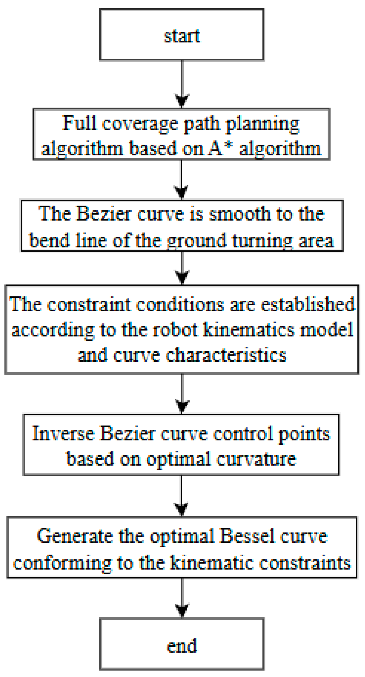
For the traditional full-coverage operation path planning algorithm, the planned path is not smooth enough and the curvature fluctuation is large, among other problems. These problems lead to the robot trajectory tracking when the driving is not smooth, leading to low operating efficiency and other issues. Therefore, this paper researches the operational requirements of orchard fertilizer robots, considers the actual environment of the orchard, proposes the full-coverage path planning algorithm based on the A* algorithm, uses the Bessel curve to smooth the folding line of the ground head turning area, establishes the constraints through the curve characteristics and kinematics model, and finally inverts the control points of the Bessel curve through the optimal curvature in order to obtain the optimal global path.
The path planning system scheme of the fertilization robot is shown in Figure 1.
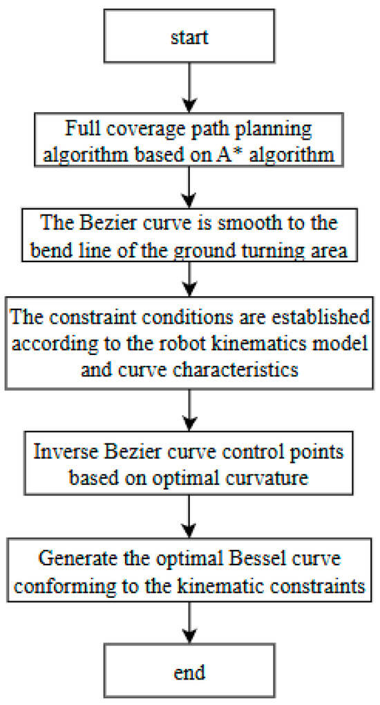
Figure 1.
System frame diagram.
2. Materials and Methods
2.1. A* Algorithm
The A* algorithm is a very commonly used heuristic search algorithm that is widely used to solve problems such as pathfinding and path planning. It is an iterative algorithm; in each iteration, it will choose the best next state according to the current state and known information until the target state is found or there is no feasible solution in the search range. The advantage of the A* algorithm is that it can find the optimal solution quickly and ensure the correctness of the optimal solution when the search space is large.
The cost function of A* algorithm is expressed as:
where indicates the node to be expanded, is the actual path cost from the starting point to the current node, is the heuristic function, and the former node estimates the generation value to the target point.
The characteristic of the cost function is that when = 0, the A* algorithm becomes a greedy algorithm, which can accelerate the solving speed but not necessarily obtain the optimal solution. When = 0, the A* algorithm becomes Dijkstra’s algorithm, which will increase the computational load of the program and lead to lower efficiency. The A* algorithm computes and simultaneously in the search process and guarantees the optimal path while considering the search efficiency.
When using the A* algorithm for path planning, the algorithm steps are divided into three steps. The first step adds the starting point to the Openlist list, sets the cost to the initial value, and initializes an empty Closelist list. The Openlist table is used to store nodes that are to be extended, and the Closelist table is used to store nodes that have been extended. The second step is iterative search. When the Openlist list is not empty, repeat the following steps: Select the node with the least cost from the Openlist list as the current node. If the current node is the target node, the search ends. Otherwise, move the current node from the Openlist list to the Closelist list and extend its neighbors. For each adjacent node, if the adjacent node is not passable or is already in the Closelist list, it is ignored. If adjacent nodes are not in the Openlist list, they are added and sorted by value. Finally, if the destination node is found, a path from the starting point to the destination point is generated by tracing back to the parent node.
2.2. Improved A* Full Coverage Path Planning Algorithm
The traditional A* algorithm belongs to “point-to-point” path planning, which is generally used to plan the shortest distance between two points and is not suitable for operation in orchards; this is because when there are many lines of fruit trees, the traditional A* algorithm will directly plan the shortest distance between the starting point and the target point and cannot cover every line of operation area. Therefore, on the premise of ensuring the effectiveness of single-row operation, this study added guide points in the front and back midpoints of each fertilization area, realized the whole plot coverage through the iterative A* algorithm, made the robot walk to the middle of the plot, and the robot planned from the starting point to the first guide point and then planned from the first guide point to the second guide point until we find the target point. The advantage of this algorithm is that it can not only achieve full coverage of orchards but also make use of the property of A* algorithm to plan the path to avoid the static obstacles in the grid map in advance so as to improve the operation efficiency. The cultivation pattern in the Qianmuyuan Garden Grape Base follows a ridge-planting approach, where grapevines are planted in a single row on each ridge, with row spacing set at 3 m.
2.3. Improved A* Path Planning Algorithm Based on Multi-Constrained Bessel Curve
The path trajectory obtained by the improved A* full coverage path planning algorithm has many problems such as too long a turning times, too many broken lines, and the path is not smooth enough. The unsmoothness of the path will cause the robot to suddenly change its direction during driving, resulting in the fertilizer robot losing control, thus reducing the work efficiency. A Bessel curve is developed based on Bernstein polynomials and is often used to smooth broken lines. In this section, a Bessel curve is used to smooth the global path planned by the improved A* algorithm under the constraints of robot kinematics.
2.3.1. Kinematic Model of Differential Steering Fertilization Robot Was Established
In the process of autonomous operation, the orchard fertilization robot has a relatively slow speed and suffers less lateral force at low speed, so it can ignore the side-slip phenomenon caused by inertia when the vehicle turns. The kinematics model of the fertilization robot is shown in Figure 2.
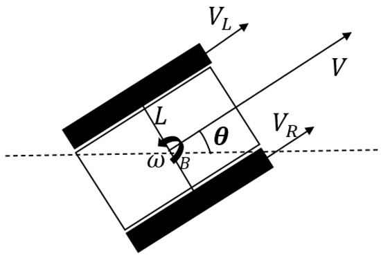
Figure 2.
Kinematics model of fertilizer robot.
In the figure: represents the left-wheel speed of the fertilizer applicator, represents the forward speed of the right wheel, represents the vehicle wheel base, that is the distance between two tracks of the fertilizer applicator, It represents the Angle between the central axis of the vehicle and the horizontal direction, that is the azimuth Angle of the fertilization robot, is the angular speed of rotation around the Z axis, expressed in rad/s, Point B is the center of the vehicle. The kinematic model is analyzed by geometry.
Forward speed is:
The turning angular velocity is:
The turning radius R is:
Steering curvature is:
Velocity relation of robot center of mass velocity in global coordinate system:
Suppose the maximum right wheel speed of a vehicle is as follows:
When the forward speed is constant, the maximum steering curvature of the vehicle is as follows:
It can be seen from the above that when the forward speed of the vehicle , the vehicle is at rest at this time, but it can turn in place and the steering curvature is infinite. When the forward speed of the vehicle , the vehicle travels in a straight line and the steering curvature is 0.
2.3.2. Bessel Curve
The Bezier curve has the following characteristics: The shape of the Bezier curve is determined by the control points, in which the first control point and the last control point are the starting point and the end point of the curve, respectively, and the control point in the middle is not above the Bezier curve. By adjusting the position and number of control points, different Bezier curves can be established. After smoothing the Bessel curve, the generated path can be closer to the theoretical driving path. This smooth processing can reduce the sharp turn of the path, thus making the trajectory tracking of the robot smoother and more efficient.
An expression for an NTH degree Bezier curve is:
where represents the parametric equation of Bessel curve, is an independent variable with the range (0,1), represents the order of the Bessel curve, is the control point on the Bezier curve, , is the starting point and the ending point, respectively, and is a Bernstein polynomial that satisfies .
The expression for solving the curvature of Bessel curve is:
where is the curvature of the Bessel curve at , is the first derivative of the Bessel curve at , is the second derivative of the Bessel curve at .
The order of the Bessel curve depends on the number of control points and can usually reach a very high order. However, when the order of the curve is too high, the influence of adjusting the control point on the curve becomes small, and the calculation amount of the program will be increased. In addition, according to the conclusion of literature [17], the numerical stability of higher-order Bessel curve is poor. To solve this numerical stability problem while satisfying the curvature constraint, Bessel curves below the third order are usually used. According to Formula (10), if curvature continuity is required, the second derivative of Bessel curve is required to be continuous, so the order of Bessel curve needs to reach more than three orders to meet the curvature continuity of the generated curve.
In summary, a third-order Bessel curve is used to smooth the transition path generated by the improved A* full coverage path planning algorithm. The specific steps of smoothing are to extract the turning point from the path generated by A* algorithm and use of the third-order Bessel curve to interpolate the smooth path segment.
2.3.3. Bessel Curve Smoothing under Multiple Constraints
When the trajectory of the orchard fertilization robot is planned to be smooth, it should be ensured that the smooth trajectory conforms to the robot’s kinematic constraints to ensure the minimum cost of robot trajectory tracking. Therefore, when the trajectory is smooth, kinematic constraints need to be added, and the trajectory curve should have the following constraints combined with the kinematic model of the fertilization robot [21]:
- (1)
- Curvature continuity constraint. Continuous curvature constraint is the key to ensure smooth turning of fertilizer robot. Curvature continuity requires the curvature changes of adjacent path segments on the path to be continuous, which can avoid the instability phenomena such as drastic turns in the tracking process of the fertilizer robot. According to the nature of the third-order Bessel curve, its second derivative is continuous, which can ensure that the trajectory planned at the turning point meets the curvature continuity constraints.
- (2)
- Slope continuity constraint. In order to smooth the global path, it is necessary to ensure the slope continuity at the connection between the Bezier curve and the straight line, so it is necessary to ensure the continuity of the first derivative at the connection of the curve. Taking the derivative of the connection between the Bezier curve and the straight line, substituting = 0 and =1, respectively (i.e., the start and end times of the Bezier curve), so that the two are equal, the junction of the third-order Bezier curve can be smooth.
The third-order Bessel curve is defined by four points, except for and , where the tangent Angle is and the tangent Angle is . There are also two control points, denoted as and in turn. Since the first derivative of the curve function is required to be continuous, the coordinates of control points and are approximately calculated by extending the line according to the known tangent Angle and the coordinates of the starting point and the end point. Let us say the length of the extended line is .
If the tangent line extends outward, is positive, and the control point coordinates are as follows:
If the tangent line extends inward, is negative, and the control point coordinates are as follows:
- (3)
- Constraints on turning radius of fertilizer robot. The turning radius constraint ensures that any part of the trajectory curve has the practical feasibility that the robot can track, and the curvature of any point on the trajectory should be less than the reciprocal of the minimum turning radius of the robot, as shown below
According to the above constraints, it is assumed that the curvature of any point in the trajectory of the ground turning region is . After the trajectory is represented by a cubic Bessel curve, the optimal method is used to solve the curve parameters under multiple constraints. The objective of optimization is the mean curvature of the curve of the ground turning region, i.e.,
By changing the control points and coordinates and changing the curve shape, the mean curvature is minimized and a smooth and continuous trajectory curve is obtained [22]. At the same time, the optimization process has the following constraints:
where: is the starting curvature of the third-order Bessel curve, is the end curvature of the third-order Bessel curve, is the curvature at the junction between the line and the starting point of the third-order Bessel curve, is the curvature of the line where it joins the end point of a third-order Bessel curve.
The gradient descent optimization algorithm [23] is used to adjust the positions of intermediate control points and to minimize the objective function . The steps of gradient descent are as follows: Calculate the gradient of the objective function with respect to the control points and , update the positions of the control points and according to the gradient direction, and repeat the above steps until the convergence condition is reached.
For each control point , the update rule can be updated according to the gradient and learning rate of the objective function, as follows:
where is the number of iterations, is the learning rate, is the gradient of the objective function relative to the control point .
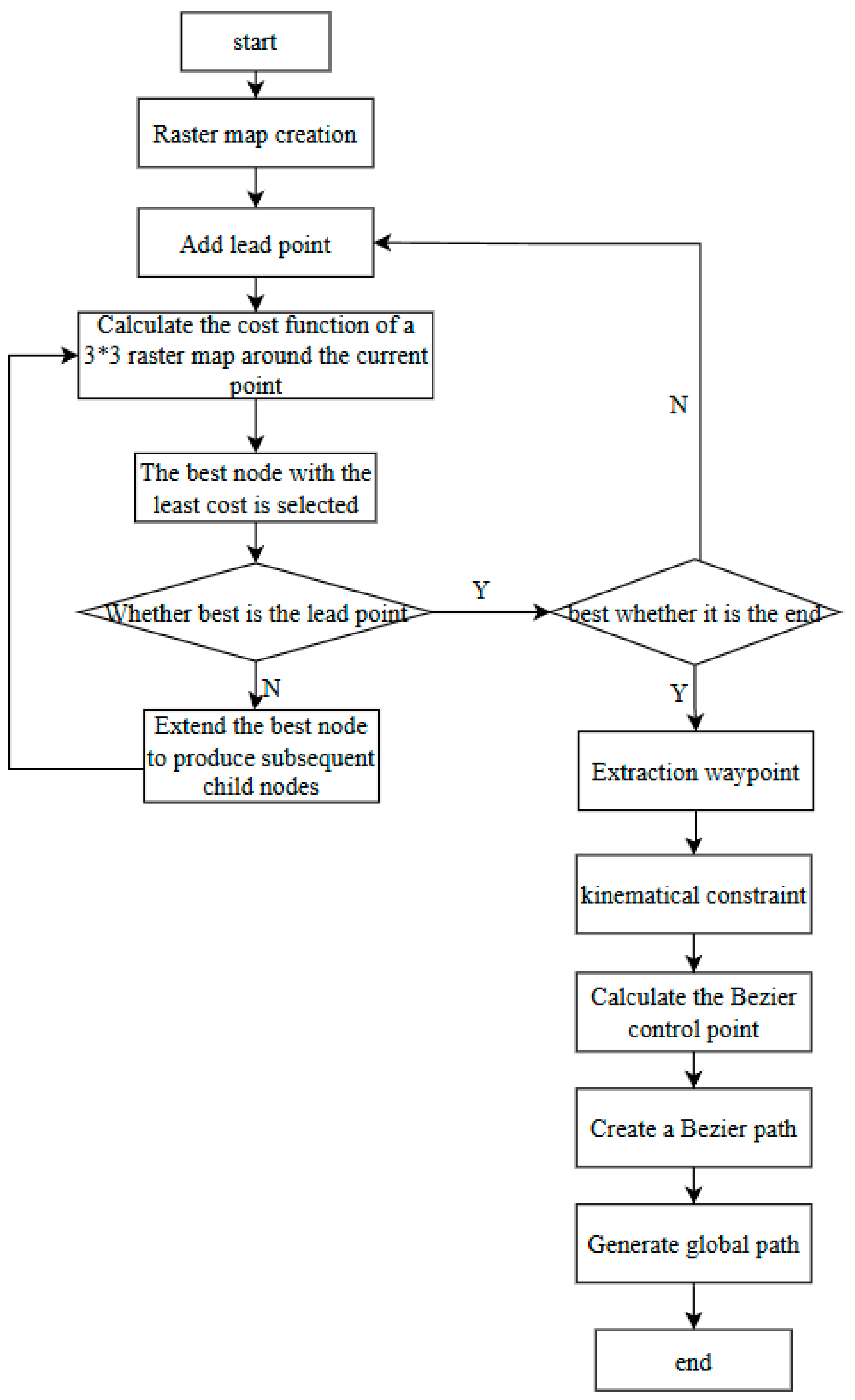
The flow chart of the improved A* algorithm based on the multi-constrained Bessel curve is shown in Figure 3.
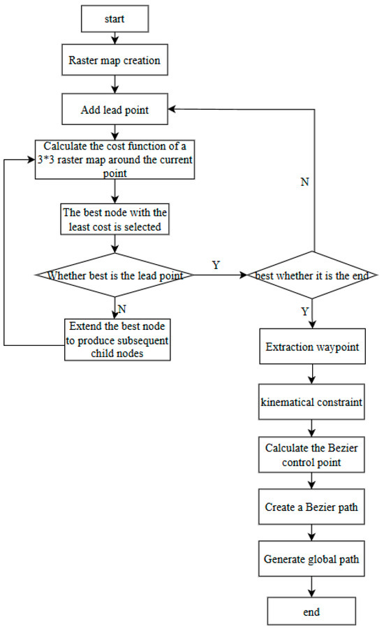
Figure 3.
Flowchart of Improved A* Algorithm Based on Multi Constraint Bessel Curve.
3. Results
3.1. Simulation Analysis
3.1.1. Static Simulation of Improved A* Algorithm Based on Multi-Constrained Bessel Curve
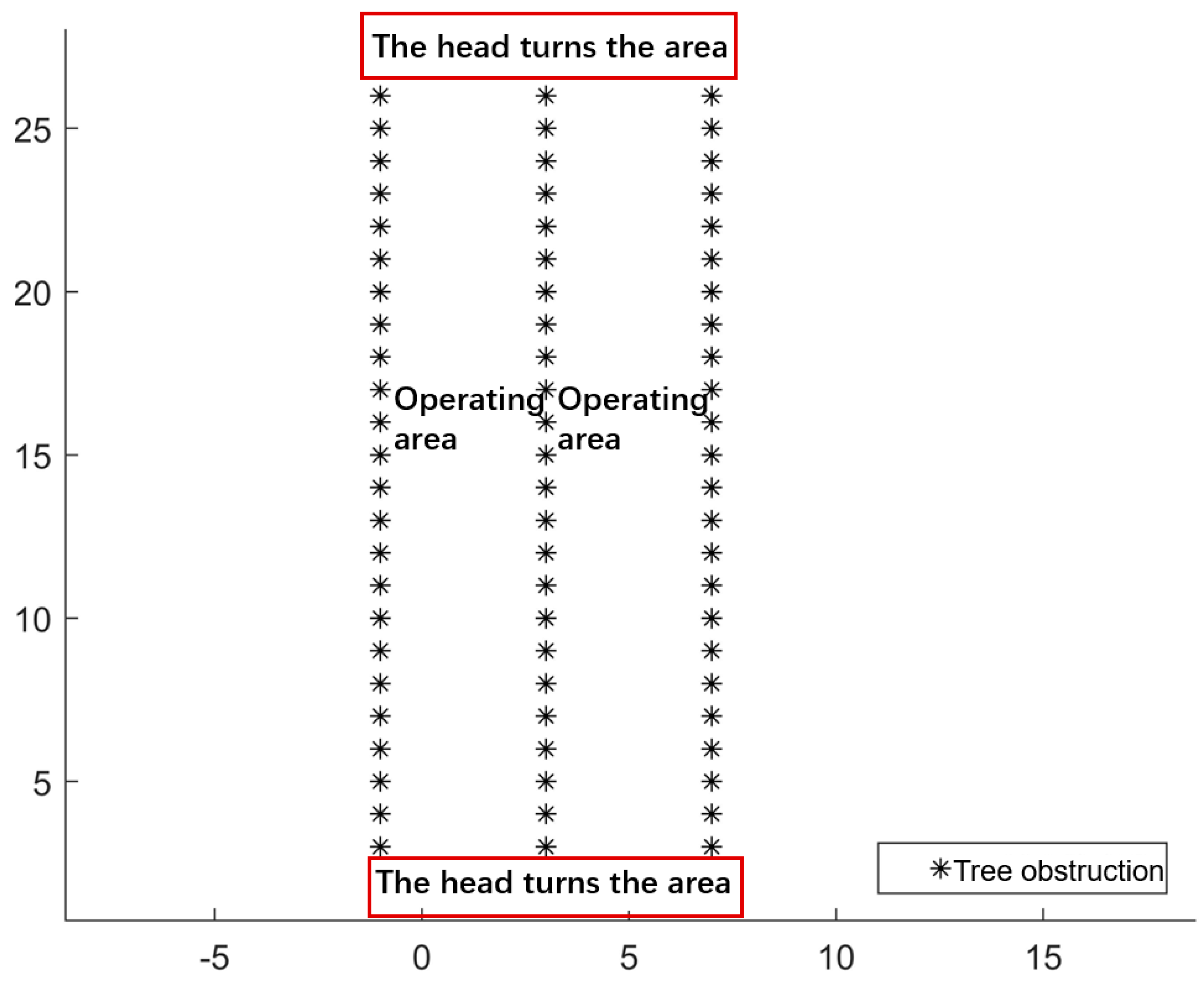
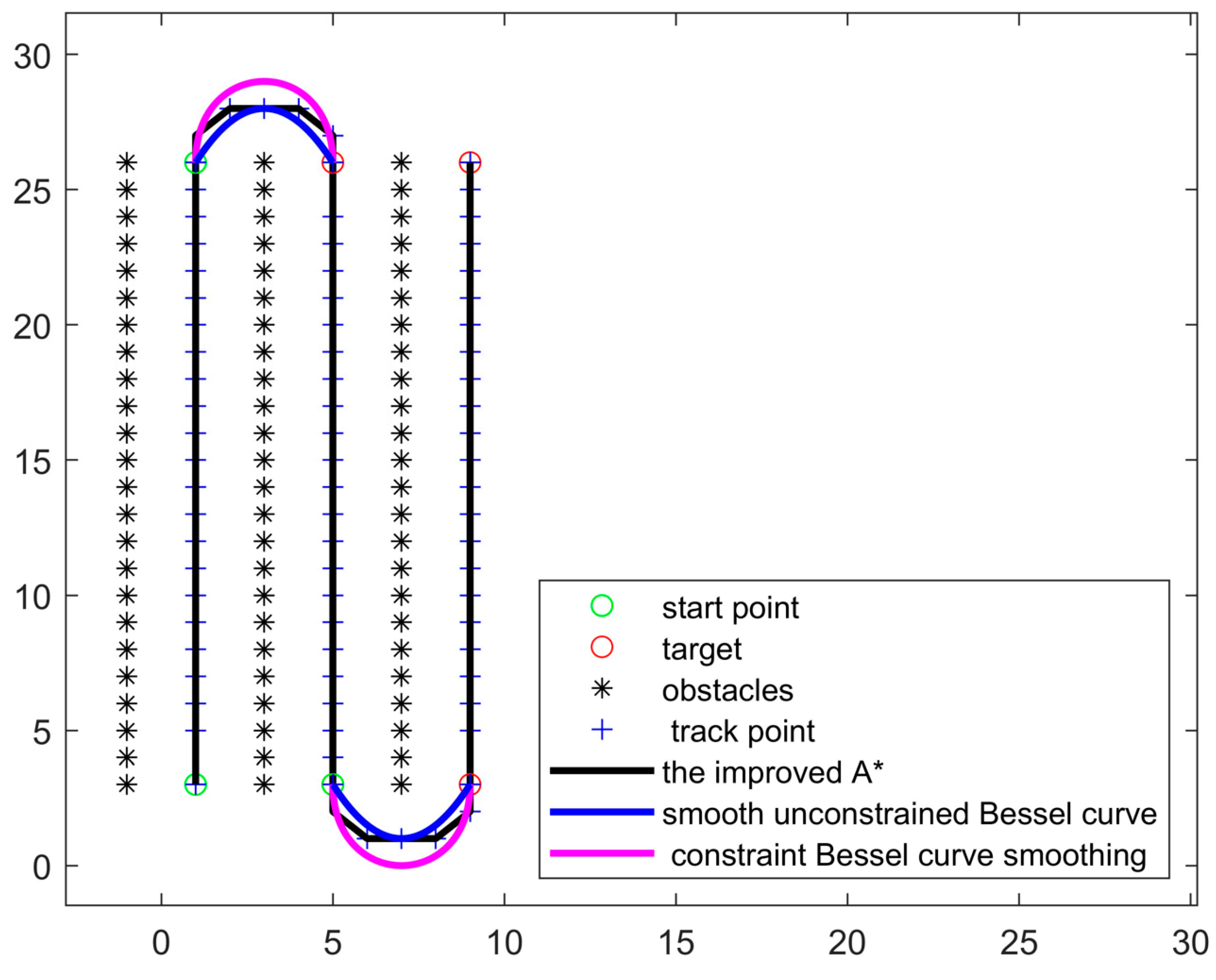
A simplified map of an orchard environment was established with MATLAB 2021a. When constructing the map, considering the safe distance traveled by the fertilizing robot, the robot is regarded as a particle, and the position of the fruit tree is properly expanded to ensure the safety of the robot during operation. The size of the map is 30 × 30 grid units, as shown in Figure 4. The positions of the fruit trees are indicated by black asterisks. There are three lines of fruit trees, and a working area is formed between the two lines of fruit trees. The end area of the fruit tree row is the head turning area, which is enclosed with a red rectangle.
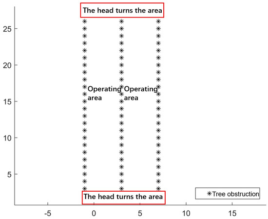
Figure 4.
Simulated Orchard Environment Map.
The starting point of the fertilization robot is set as (1,3) and the target point is set as (9,26), so that the operation path can achieve full coverage of the operation area. The improved A*, unconstrained Bessel curve, and multi-constrained Bessel curve full coverage path planning algorithms are used for global path planning, and the results obtained in the raster map are shown in Figure 5.
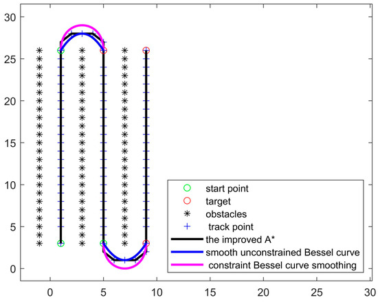
Figure 5.
A* Algorithm before and after Bessel Curve Optimization.
According to the land turning area in Figure 5, it can be found that the A* algorithm optimized with a Bezier curve is smoother in the land turning area and more suitable for orchard scene operations. However, the slope of the global path optimized with unconstrained Bezier curve changes at the junction of the straight line and the U-turn path, resulting in the path being not smooth. The curvature diagram of the multi-constrained Bessel curve is shown in Figure 6, and the slope diagram is shown in Figure 7.
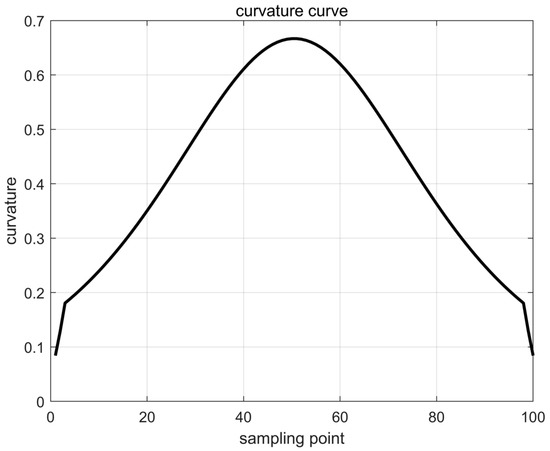
Figure 6.
Curvature diagram of multiple constrained Bessel curves.
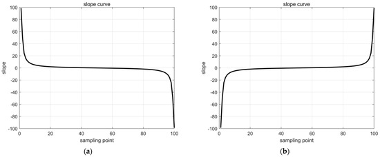
Figure 7.
Slope diagram of multi-constrained Bessel curve: (a) traditional gate-type path; (b) improved gate-type path.
It can be seen from Figure 6 that the curvature of the multi-constrained Bessel curve satisfies the curvature continuity constraint.
It can be seen from Figure 7 that the slopes of both ends of the multi-constrained Bessel curve are the same as the slopes of the lines connected at both ends, satisfying the slope continuity constraint.
The minimum operating speed of the orchard fertilization robot is generally 0.5 m/s. As can be seen from Equation (18), the curve should meet the constraints of turning radius, and the maximum curvature should not exceed 1.307. As can be seen from Figure 6, the maximum curvature is 0.66, so the multi-constraint Bessel curve meets the constraints of turning radius.
3.1.2. Dynamic Simulation of Improved A* Algorithm Based on Multi-Constrained Bessel Curve
According to the simulated orchard environment map established above, as shown in Figure 4, the starting point of the fertilization robot is set as (1,3), and the target point is set as (5,3). Multi-constrained Bessel curve, unconstrained Bessel curve, improved A* full coverage, and comb full coverage path planning algorithms were used for planning, and the planned path was tracked using the improved pure tracking algorithm [24,25,26,27] proposed in Section 2. Lateral deviation of different paths and robot course Angle fluctuation were compared to judge the quality of the path.
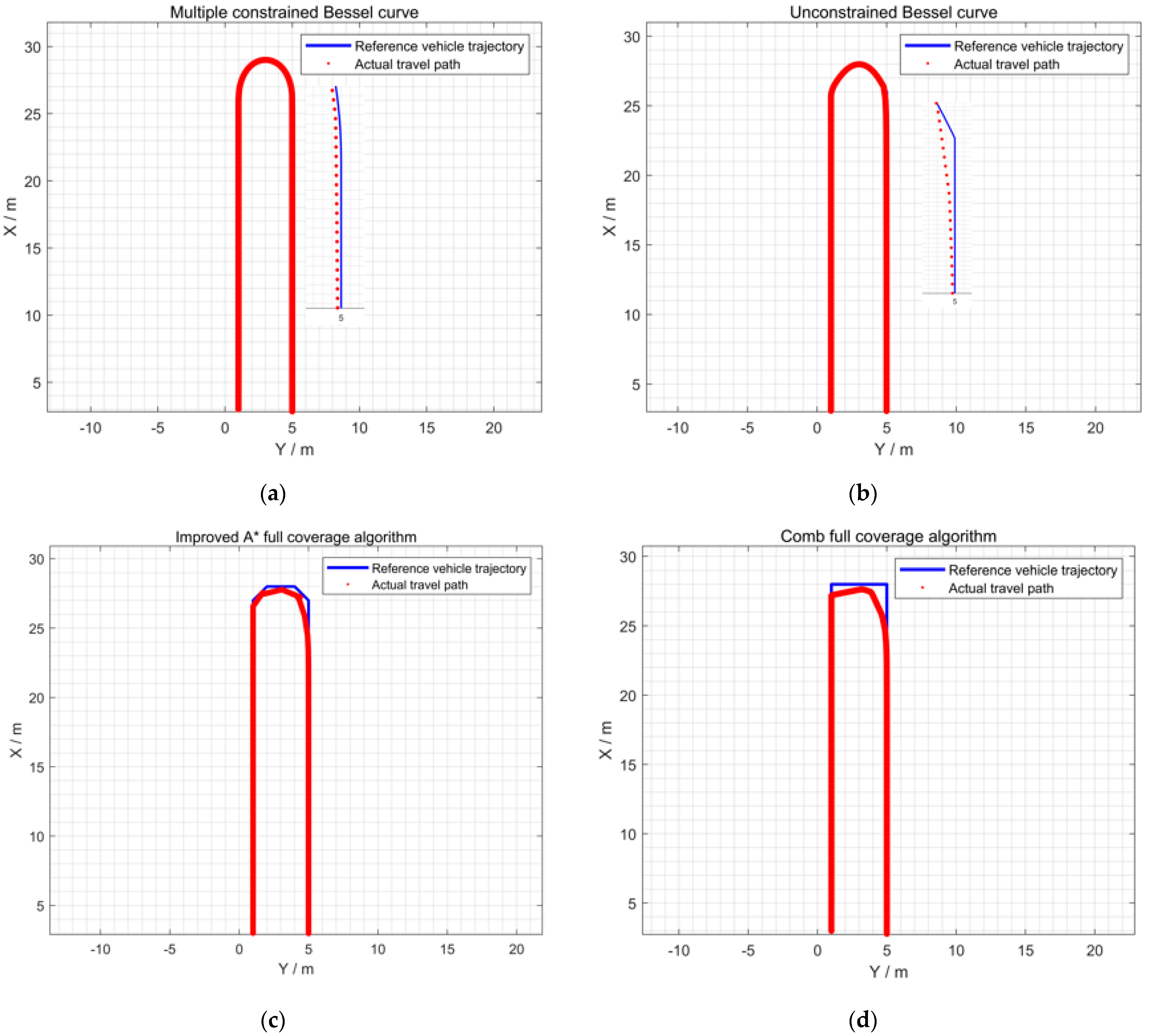
The trajectory tracking curves generated by the four algorithms were simulated. The speed of the robot was set to 1.5 m/s, the basic forward looking distance was set to = 1 m, the speed control gain coefficient of the improved pure tracking algorithm was set to = 1, and the integral adjustment coefficient was set to = 0.5. The trajectory tracking diagram is shown in Figure 8, course Angle diagram is shown in Figure 9, and lateral deviation is shown in Figure 10. The lateral deviation data obtained from the test are shown in Table 1.
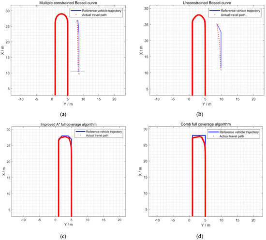
Figure 8.
Trajectory tracking diagram of four algorithms: (a) multi-constrained Bessel optimization; (b) unconstrained Bessel optimization; (c) Improved A* full coverage algorithm; (d) Comb full coverage algorithm.
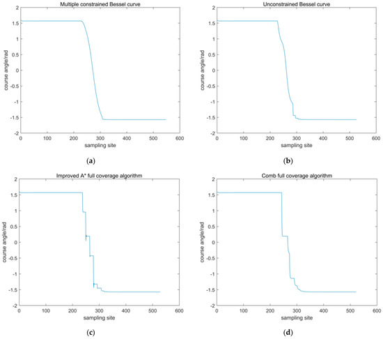
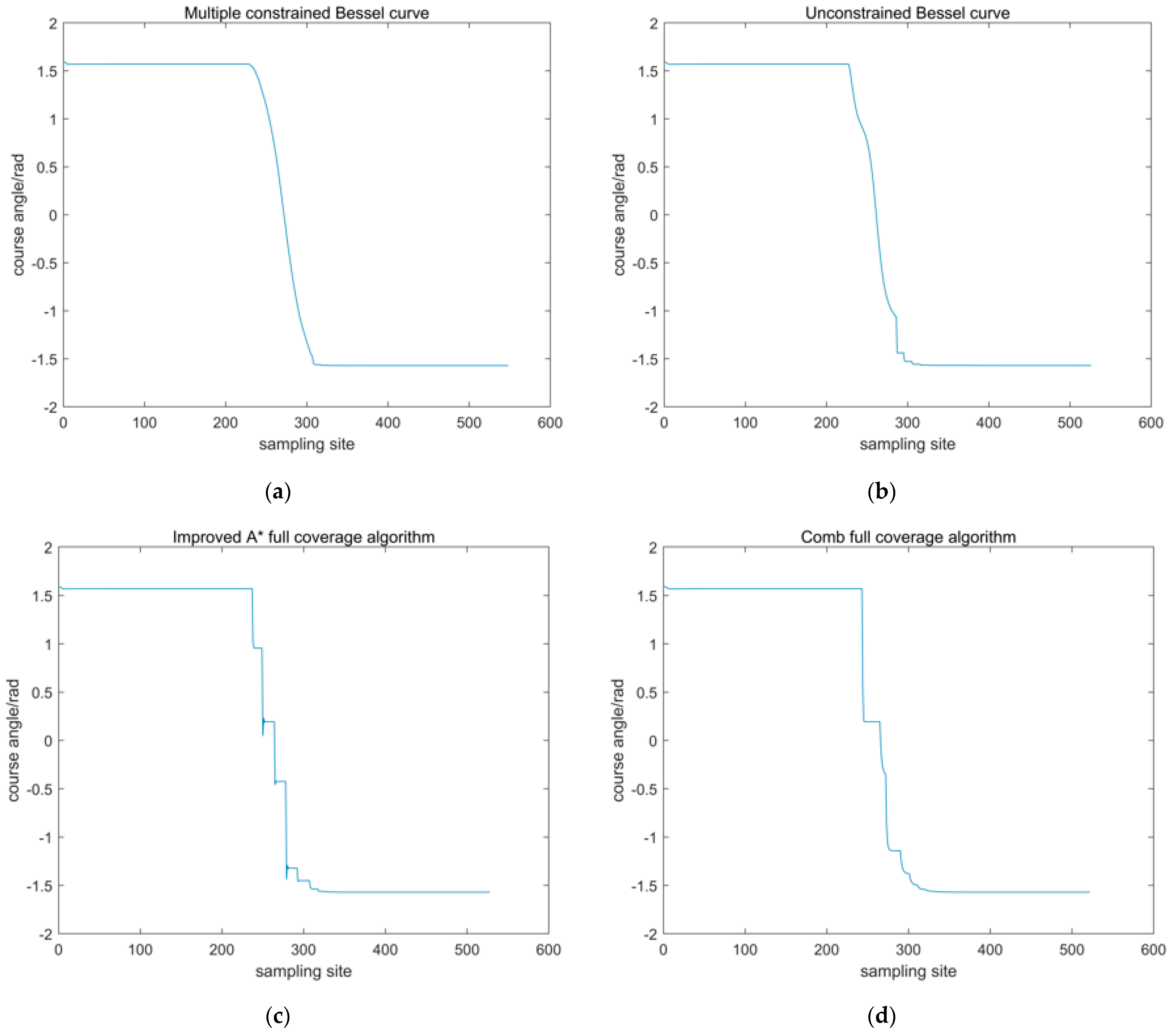
Figure 9.
Course Angle diagram of four algorithms: (a) multi-constrained Bessel optimization; (b) unconstrained Bessel optimization; (c) Improved A* full coverage algorithm; (d) Comb full coverage algorithm.
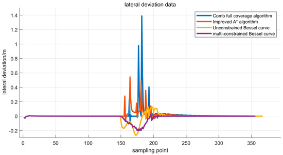
Figure 10.
Trajectory tracking lateral deviation results under four full coverage planning algorithms.

Table 1.
Trajectory tracking lateral deviation data under five full coverage planning algorithms.
According to the above experiments, we can know the following:
As can be seen from Figure 8c,d and Figure 9c,d, when the path planned by the improved A* full coverage and comb full coverage path planning algorithm is tracked, the path turning amplitude planned by the algorithm is large and not smooth, resulting in abrupt heading Angle and poor track tracking effect when the robot entered the ground turning area. The robot rides unsmoothly. It can be seen from Figure 10 and Table 1 that the lateral bias of these two algorithms is much greater than that of the other two algorithms.
According to Figure 8a,b and Figure 9a,b, it can be seen that the path planned by the multi-constrained Bessel curve and unconstrained Bessel curve optimization algorithm with full coverage of the path planning algorithm is relatively smooth, and the robot’s heading Angle has no major sudden change as a whole. Lateral deviation is shown in Figure 10. It can be seen that when tracking, the multi-constrained Bessel curve algorithm plans the path, when entering the U-turn path, the lateral deviation fluctuates little, and the robot rides more smoothly. When exiting the curve, the lateral deviation of the optimization algorithm of unconstrained Bessel curve fluctuates greatly, which affects the robot’s ride stability.
As can be seen from Table 1, compared with the optimization algorithm of unconstrained Bessel curve, the average transverse deviation of the multi-constrained Bessel curve is reduced by 0.0029 m, and the maximum transverse deviation is reduced by 0.0671 m.
In summary, by adding three Bezier curve optimization and kinematic constraints to the improved full-coverage A* algorithm, the lateral deviation can be effectively reduced, and the ride stability of the robot can be increased.
3.2. Real Machine Test
3.2.1. Test Platform
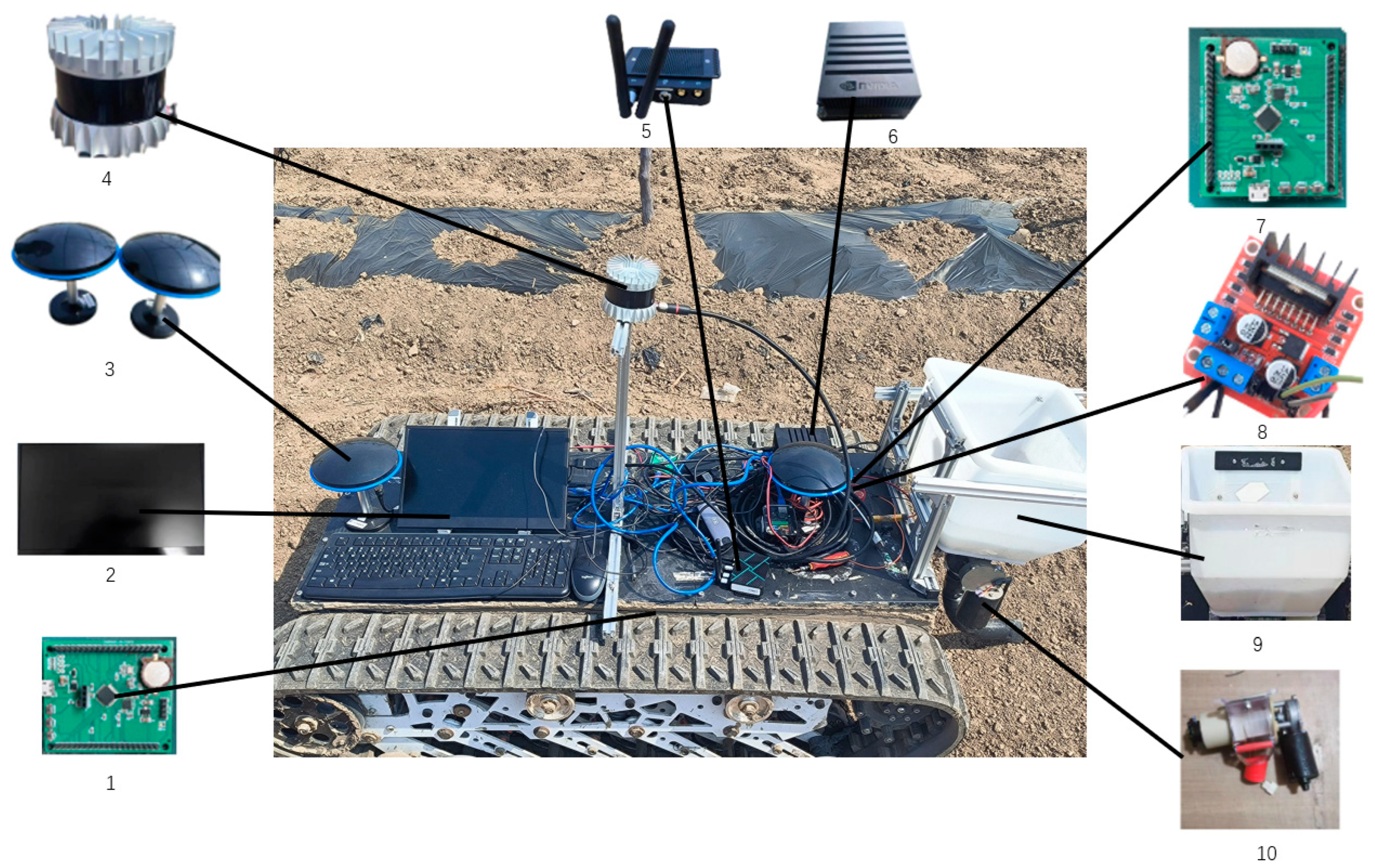
The algorithm in this paper verifies that the orchard fertilization robot with differential steering chassis is used as the test platform. The orchard fertilization robot is composed of a tracked differential steering chassis and an autonomous operating system based on artificial intelligence processor, as shown in Figure 11. The hardware of the autonomous operating system includes the STM32 underlying control driver board, NVIDIA artificial intelligence processor, GNSS-RTK receiver, 3D LiDAR, STM32 fertilizer motor driver board, and fertilizer equipment. Robot communication and driving code is written based on ROS platform [28,29] and the planned path is loaded into the pre-programmed container; the planned path and actual driving trajectory can be observed through the visualization software RVIZ1.12.
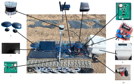
Figure 11.
Orchard fertilization robot. 1: STM32 bottom control driver board; 2: Display screen; 3: Positioning directional antenna; 4: 64 line LiDAR; 5: GNSS-RTK positioning receiver; 6: Artificial intelligence processor; 7: STM32 fertilizer discharge motor drive board; 8: L298N motor control module; 9: Fertilizer can; 10: Fertilizer discharge motor.
The autonomous operation of the orchard fertilization robot needs to receive stable positioning signals so the site needs to be without obvious shelter. The site was selected as the thousand mu garden grape base in Huantai County, Zibo City, Shandong Province. First, the track tracking path is selected in the test area. The track tracking path should consist of two parts: one is the straight path of the fertilization area and the other is the U-turn path of the field head turning area. In the global path planned by the two planning algorithms, the starting point is 30 m from the end of the current tree line, and the turning path 30 m from adjacent tree lines is selected as the target point and the tracking path of the test. A pure tracking algorithm is used to track the trajectory planned by the traditional comb algorithm and the algorithm in this paper.
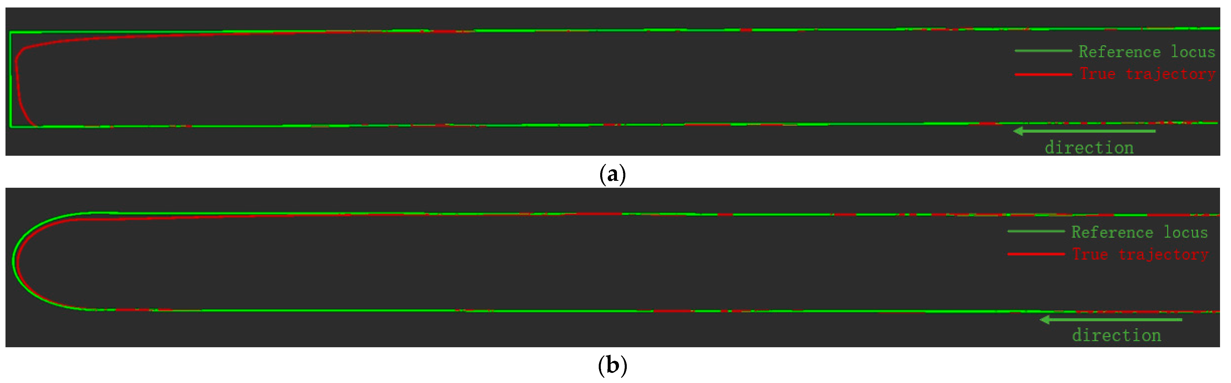
After the fertilizer robot reaches the end point and stops, the RVIZ in ROS shows the trajectory. The track tracking diagram of the path planned by the fertilization robot according to the two algorithms is shown in Figure 12.
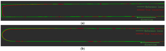
Figure 12.
The trajectory tracking graph of two path planning algorithms: (a) Comb full coverage algorithm; (b) An improved A* algorithm based on multi-constraint Bessel.
3.2.2. Experimental Design
The autonomous operation of the orchard fertilization robot needs to receive stable positioning signals, so the site needs to be without obvious shelter. The site was selected as the thousand mu garden grape base in Huantai County, Zibo City, Shandong Province. Firstly, the track tracking path is selected in the test area. The track tracking path should consist of two parts, one is the straight path of the fertilization area and the other is the U-turn path of the field head turning area. In the global path planned by the two planning algorithms, the starting point is 30 m from the end of the current tree line, and the turning path 30 m from adjacent tree lines is selected as the target point and the tracking path of the test. A pure tracking algorithm is used to track the trajectory planned by the traditional comb algorithm and the algorithm in this paper.
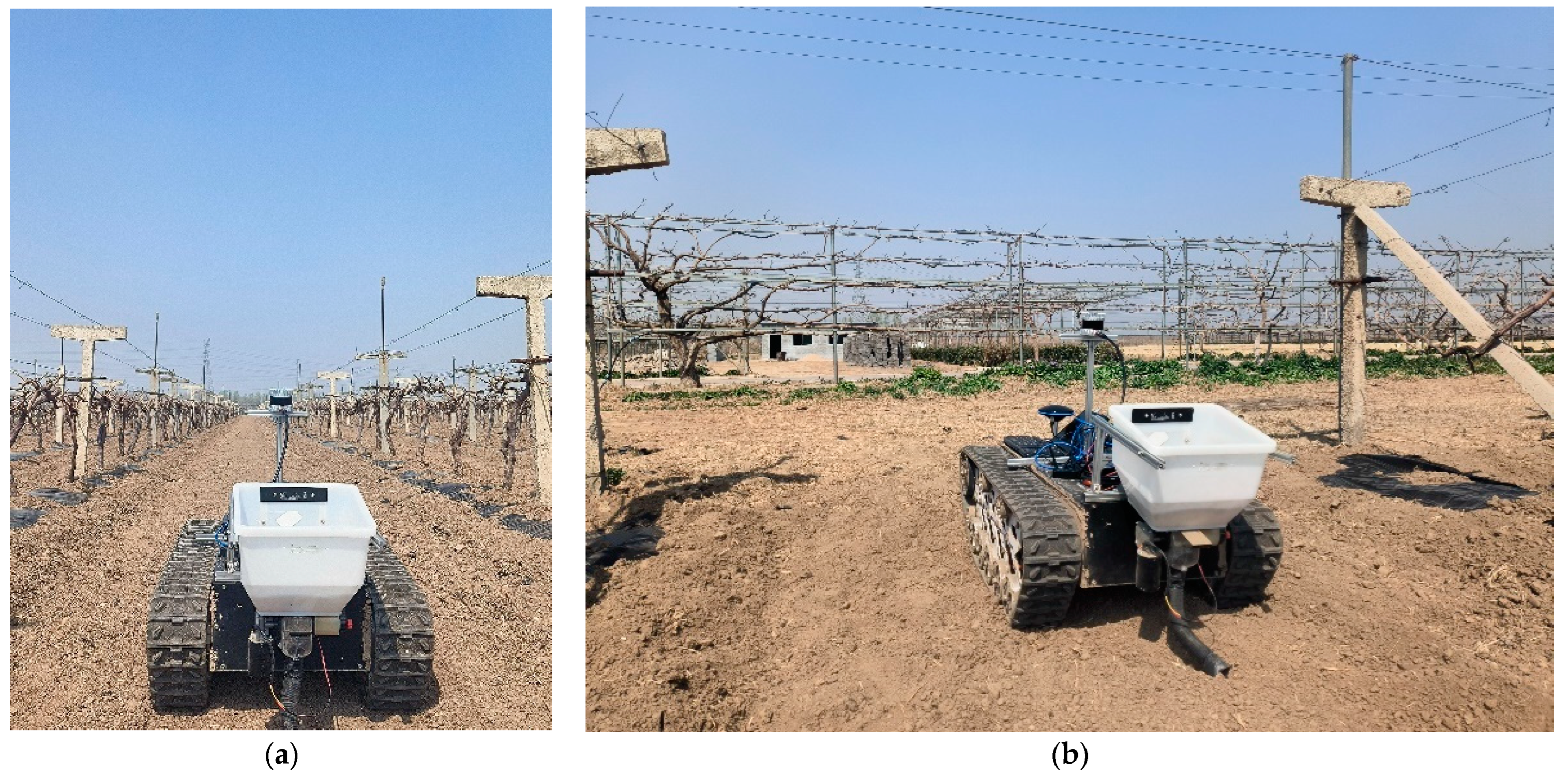
After the fertilizer robot reaches the end point and stops, the RVIZ in ROS shows the trajectory. The track tracking diagram of the path planned by the fertilization robot according to the two algorithms is shown in Figure 12. The track tracking test diagram of orchard fertilization robot is shown in Figure 13.

Figure 13.
Experimental diagram of trajectory tracking for orchard fertilization robot: (a) Starting point; (b) Entry into the ground turning area.
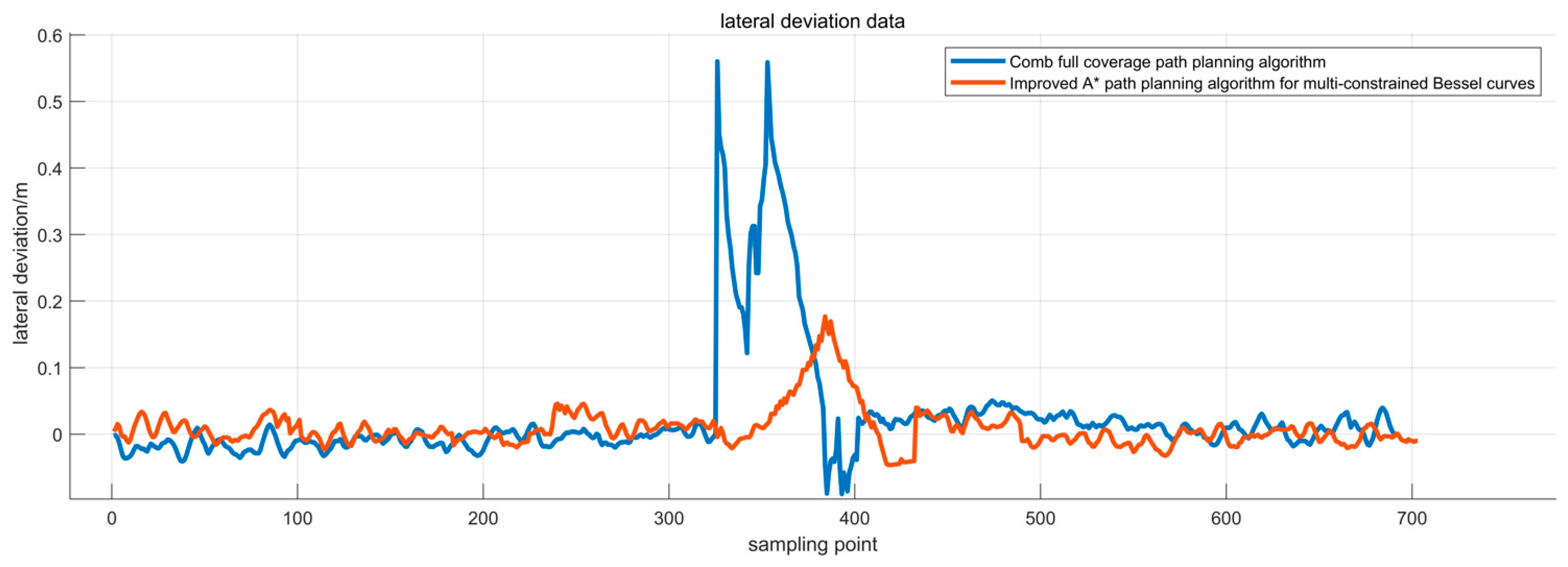
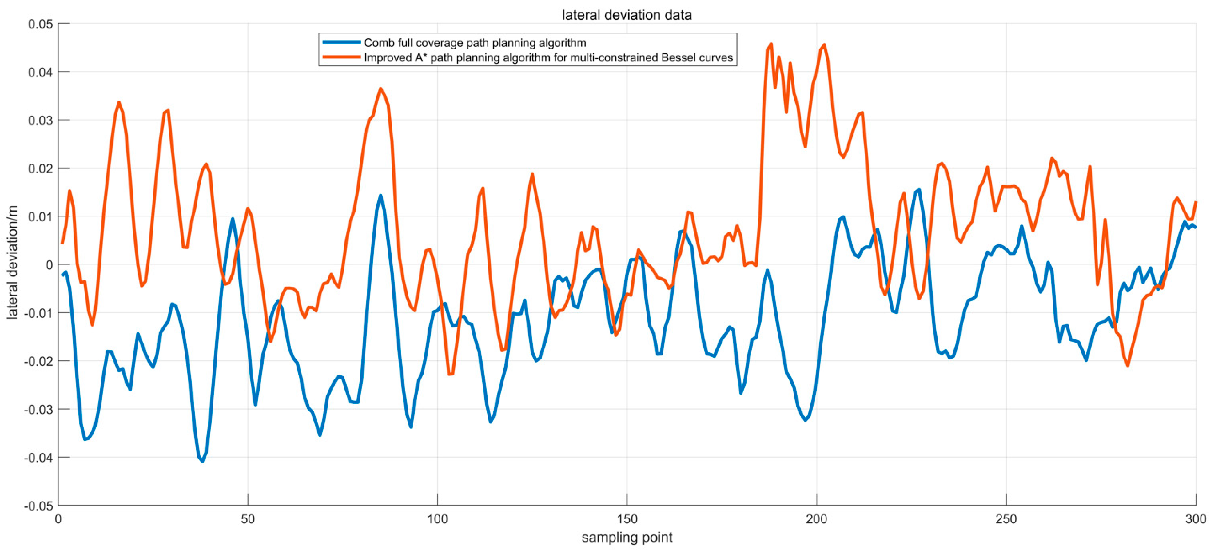
By tracking the paths generated by the two path planning algorithms, the lateral deviation of the sampling points in the process is saved as txt format, and the txt format file is imported into MATLAB to display the trajectory tracking error of the two planning algorithms. The transverse deviation results of the overall path of track tracking are shown in Figure 14, and the transverse deviation results of the straight line part of the fertilization area are shown in Figure 15. The average and maximum lateral deviation parameters under the two algorithms are shown in Table 2.

Figure 14.
Comparison of lateral tracking deviation between two algorithms for path planning.
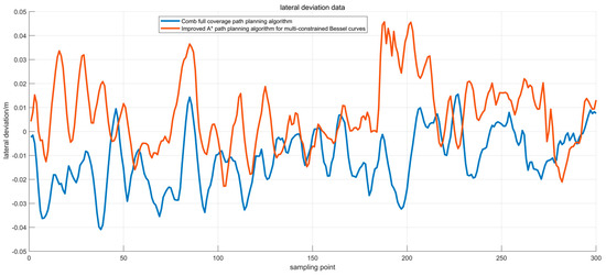
Figure 15.
Tracking lateral deviation of two algorithms in straight line region.
Table 2.
Lateral Deviation of Two Planning Paths under Improved Pure Tracking Algorithm.
According to the above tests:
As can be seen from Figure 15, when the orchard fertilizing robot uses the improved pure tracking algorithm for linear tracking, the horizontal deviation is small, with an average horizontal deviation of 0.0157 m and a maximum horizontal deviation of 0.0457 m, which meets the requirements for autonomous operation of the fertilizing robot.
As can be seen from Figure 14, when the orchard fertilization robot enters the U-turn path, the path planned by the comb full coverage path planning algorithm has a large lateral deviation from the track of the reference vehicle, and the steering amplitude of the robot fluctuates greatly during the tracking process, which affects the smoothness of the robot. As can be seen from Figure 12a, the curvature of the turn-around path generated by the comb full coverage path planning algorithm is discontinuous and does not conform to the robot kinematics constraints, resulting in large turn-around fluctuation and lateral deviation when the robot tracks the next target point. In addition, due to the large lateral deviation, the robot cannot quickly fit the straight path when exiting the curve.
As can be seen from Figure 12b and Figure 14, when the orchard fertilization robot enters the U-turn path, the overall lateral deviation is small when tracking the path planned by the improved A* algorithm based on the multi-constrained Bessel curve, and the steering amplitude of the robot fluctuates steadily during the tracking process. When the robot exits the curve, it can quickly fit the straight path. Ensure the autonomous operation efficiency of fertilizer robot.
It can be seen from the analysis of test data in Table 2 that compared with the comb full coverage path planning algorithm, the average lateral deviation of the U-turn path generated by the improved A* path planning algorithm tracking the multi-constrained Bessel curve is reduced by 0.1499 m, and the maximum lateral deviation is reduced by 0.8232 m.
Based on the above experimental analysis, it can be seen that the global path generated by the improved A* algorithm based on the multi-constraint Bessel curve meets the requirements of full coverage and smoothness and satisfies the autonomous operation requirements of orchard fertilization robots. The improved pure tracking algorithm was used to track the path. When the linear path was tracked in the fertilization area, the average lateral deviation was 0.0157 m and the maximum lateral deviation was 0.0457 m; when the U-turn path was tracked, the average lateral deviation was 0.1081 m and the maximum lateral deviation was 0.1768 m, and the steering amplitude fluctuated little and the ride was stable. To meet the requirements of autonomous operation of orchard fertilization robot.
4. Conclusions
In this study, the following improvements are made relative to the traditional algorithm. (1) Aiming at the problem that the traditional A* algorithm is unable to perform full-coverage path planning in the orchard environment, an iterative algorithm is added so that the A* algorithm can perform full-coverage planning. (2) Aiming at the autonomous driving process of fertilizer robot in orchard environment, an improved A∗ algorithm based on multi-constraint Bessel curves is proposed, which establishes multi-constraints by combining the minimum turning radius constraints of fertilizer robot and curvature constraints, establishes a mathematical model with the minimum of the mean curvature as the optimization objective, and solves the problem. The maximum curvature of the generated trajectory is 0.66 m−1, which greatly reduces the trajectory curvature compared with the initial A* algorithm and the cubic Bessel algorithm and conforms to the kinematic constraints of the orchard fertilizer robot. (3) The tracking test shows that the orchard fertilizer robot can track the path generated by the orchard driving path planning algorithm well, with an average lateral error of 0.225 m and a standard deviation of 0.031 m, which meets the requirements for the driving accuracy of the orchard fertilizer robot.
5. Discussion
In this paper, the path planning and trajectory tracking system for the autonomous operation of orchard fertilizer robots is researched and the orchard fertilizer robot is built. The research results have improved the reasonableness of the global path planning of the robot to a certain extent and increased the accuracy of trajectory tracking, but there is still room for improvement in the orchard fertilizer robot path planning system. This paper achieves a better global path planning but it does not achieve local path planning for the fertilizer robot and it does not consider the obstacle avoidance function. This paper is for standardized orchard path planning, and did not consider the complex rugged scene of the orchard in thinking about how to carry out path planning, so the subsequent need for multi-scenario orchard environment of global and local path planning research is needed to improve the adaptability of orchard fertilizer robot.
Author Contributions
Conceptualization, F.K., Y.L. and B.L.; methodology, F.K.; software, B.L.; validation, X.H., F.K. and H.S.; formal analysis, H.S.; investigation, L.Y.; resources, L.Y.; data curation, J.L.; writing—original draft preparation, L.L.; writing—review and editing, Y.L. and F.K.; supervision, F.K.; project administration, B.L.; funding acquisition, B.L. All authors have read and agreed to the published version of the manuscript.
Funding
This study obtained: Shandong Province to introduce top talents “One thing, one discussion” special project (Lu Government Office Zi [2018] No. 27) and Zibo City key research and development program funding project (No. 2019ZBXC053).
Institutional Review Board Statement
Not applicable.
Data Availability Statement
We did not use an open data set, and most of the data generated in the paper are the positioning data in the trajectory tracking process of the robot and the planned reference trajectory points.
Conflicts of Interest
The authors declare no conflicts of interest.
References
- Fu, Q.; Mei, J.; Li, L.; Wang, J.; Wang, H. Design of Intelligent Level Switch for Water and Fertilizer Integrated Intelligent Control Equipment. Trans. Chin. Soc. Agric. Mach. 2015, 46 (Suppl. S1), 108–115. [Google Scholar]
- Sang, Y.; Chen, X.; Chen, Q.; Tao, J.; Fan, Y. A route planning for oil sample transportation based on improved A* algorithm. Sci. Rep. 2023, 13, 22041. [Google Scholar] [CrossRef] [PubMed]
- Cai, B.; Li, M.; Yang, H.; Wang, C.; Chen, Y. State of Charge Estimation of Lithium-Ion Battery Based on Back Propagation Neural Network and AdaBoost Algorithm. Energies 2023, 16, 7824. [Google Scholar] [CrossRef]
- Li, J.; Yu, C.; Zhang, Z.; Sheng, Z.; Yan, Z.; Wu, X.; Zhou, W.; Xie, Y.; Huang, J. Improved A-Star Path Planning Algorithm in Obstacle Avoidance for the Fixed-Wing Aircraft. Electronics 2023, 12, 5047. [Google Scholar] [CrossRef]
- Feng, Y.; Zhang, W.; Zhu, J. Application of an Improved A* Algorithm for the Path Analysis of Urban Multi-Type Transportation Systems. Appl. Sci. 2023, 13, 13090. [Google Scholar] [CrossRef]
- Zhang, M.; Li, X.; Wang, L.; Jin, L.; Wang, S. A Path Planning System for Orchard Mower Based on Improved A* Algorithm. Agronomy 2024, 14, 391. [Google Scholar] [CrossRef]
- Liao, T.; Chen, F.; Wu, Y.; Zeng, H.; Ouyang, S.; Guan, J. Research on Path Planning with the Integration of Adaptive A-Star Algorithm and Improved Dynamic Window Approach. Electronics 2024, 13, 455. [Google Scholar] [CrossRef]
- Zhu, J.; Li, J.; Li, J.; Zhang, Z. Path planning of POL-Robot based on improved A* algorithm. Mech. Electr. Eng. Technol. 2022, 51, 1–5. [Google Scholar]
- Wang, Z.; Chen, X. Unmanned boat path planning algorithm based on improved, A*. DWA J. Sens. Technol. 2021, 34, 249–254. [Google Scholar]
- Gino, G.; David, F.; Nazik, Ö.; Liakopoulos, S.; Papanastassiou, D.; Faranda, C. Quaternary E-W Extension Uplifts Kythira Island and Segments the Hellenic Arc. Tectonics 2022, 41, e2022TC007231. [Google Scholar]
- Song, J.; Wu, J.; Wang, X.; Duan, Z.; Wang, X.; Lu, S. Accurate classification of power quality disturbance based on 3D visualized spiral curve and hybrid ER-MVCNN model. Measurement 2024, 231, 114654. [Google Scholar] [CrossRef]
- Gómez-Bravo, F.; Cuesta, F.; Ollero, A.; Viguria, A. Continuous curvature path generation based on β-spline curves for parking manoeuvres. Robot. Auton. Syst. 2008, 56, 360–372. [Google Scholar] [CrossRef]
- Li, J.; Liu, C. Smoothing Connected Bezier Curves and Surfaces through Optimal Adjustment of the Control Points. IAENG Int. J. Comput. Sci. 2023, 50, 1098–1107. [Google Scholar]
- Zhihao, Z.; Xiaodong, L.; Boyu, F. Research on obstacle avoidance path planning of UAV in complex environments based on improved Bézier curve. Sci. Rep. 2023, 13, 16453. [Google Scholar]
- Chojnacki, B.; Schynol, K.; Halek, M.; Muniak, A. Sustainable Perforated Acoustic Wooden Panels Designed Using Third-Degree-of-Freedom Bezier Curves with Broadband Sound Absorption Coefficients. Materials 2023, 16, 6089. [Google Scholar] [CrossRef] [PubMed]
- Takafumi, S.; Norimasa, Y. Curvature monotonicity evaluation functions on rational Bézier curves. Comput. Graph. 2023, 114, 219–228. [Google Scholar]
- Choi, J.W.; Curry, R.E.; Elkaim, G.H. Curvature-continuous trajectory generation with corridor constraint for autonomous ground vehicles. In Proceedings of the 49th IEEE Conference on Decision and Control (CDC), Atlanta, GA, USA, 15–17 December 2010; IEEE: Piscataway, NJ, USA, 2010; pp. 7166–7171. [Google Scholar]
- Zhao, W.; Zhou, D. Improved path planning algorithm based on A* and third-order Bézier curve fusion. J. Anhui Univ. Technol. (Nat. Sci. Ed.) 2023, 40, 333–338. [Google Scholar]
- Lu, E.; Lin, W.; Liu, Y. Research on intelligent forklift pallet picking path planning based on B-spline curves. Trans. Chin. Soc. Agric. Mach. 2019, 50, 394–402. [Google Scholar]
- Zhang, W.; Liu, Y.; Zhang, C.; Zhang, L.; Xia, Y. Real-time path planning for greenhouse robots based on directional A* algorithm. Trans. Chin. Soc. Agric. Mach. 2017, 48, 22–28. [Google Scholar]
- Shen, Y.; Liu, Z.; Liu, H.; Du, W. Path planning method for orchard spray Robot based on Multiple Constraints. Trans. Chin. Soc. Agric. Mach. 2023, 54, 56–67. [Google Scholar]
- Sun, W.; Tang, G.; Hauser, K. Fast UAV trajectory optimization using bilevel optimization with analytical gradients. In Proceedings of the 2020 American Control Conference (ACC), Denver, CO, USA, 1–3 July 2020; IEEE: Piscataway, NJ, USA, 2020; pp. 82–87. [Google Scholar]
- Yang, F.; Li, W.; Yan, T.-H. Path planning Algorithm of Mobile Robot based on gradient Optimization. Mod. Electron. Tech. 2019, 46, 99–104. [Google Scholar]
- Fue, K.; Porter, W.; Barnes, E.; Li, C.; Rains, G. Autonomous Navigation of a Center-Articulated and Hydrostatic Transmission Rover using a Modified Pure Pursuit Algorithm in a Cotton Field. Sensors 2020, 20, 4412. [Google Scholar] [CrossRef] [PubMed]
- Wu, G.; Wang, G.; Bi, Q.; Wang, Y.; Fang, Y.; Guo, G.; Qu, W. Research on unmanned electric shovel autonomous driving path tracking control based on improved pure tracking and fuzzy control. J. Field Robot. 2023, 40, 1739–1753. [Google Scholar] [CrossRef]
- Wei, Y.; Li, H.; Zhou, Z.; Chen, D. Driving Path Tracking Strategy of Humanoid Robot Based on Improved Pure Tracking Algorithm. IAENG Int. J. Appl. Math. 2024, 54, 286–297. [Google Scholar]
- Kayacan, E.; Ramon, H.; Saeys, W. Towards agrobots: Identification of the yaw dynamics and trajectory tracking of an autonomous tractor. Comput. Electron. Agric. 2015, 115, 78–87. [Google Scholar] [CrossRef]
- Bai, W.; Cao, Q.; Wang, P.; Chen, P.; Leng, C.; Pan, T. Modular design of a teleoperated robotic control system for laparoscopic minimally invasive surgery based on ROS and RT-Middleware. Ind. Robot. 2017, 44, 596–608. [Google Scholar] [CrossRef]
- MathWorks. MathWorks Introduces Robotics System Toolbox for Complete Integration with Robot Operating System ROS, Version 2015a; Biotech Business Week; MathWorks: Natick, MA, USA, 2015. [Google Scholar]


Disclaimer/Publisher’s Note: The statements, opinions and data contained in all publications are solely those of the individual author(s) and contributor(s) and not of MDPI and/or the editor(s). MDPI and/or the editor(s) disclaim responsibility for any injury to people or property resulting from any ideas, methods, instructions or products referred to in the content. |
© 2024 by the authors. Licensee MDPI, Basel, Switzerland. This article is an open access article distributed under the terms and conditions of the Creative Commons Attribution (CC BY) license (https://creativecommons.org/licenses/by/4.0/).