
Genome-Wide Composite Interval Mapping Reveal Closely Linked Quantitative Genes Related to OJIP Test Parameters under Chilling Stress Condition in Barley

Abstract
1. Introduction
2. Results
2.1. Evaluation of OJIP Test Parameters (Quantitative Data)
2.1.1. Descriptive Statistics
2.1.2. ANOVA
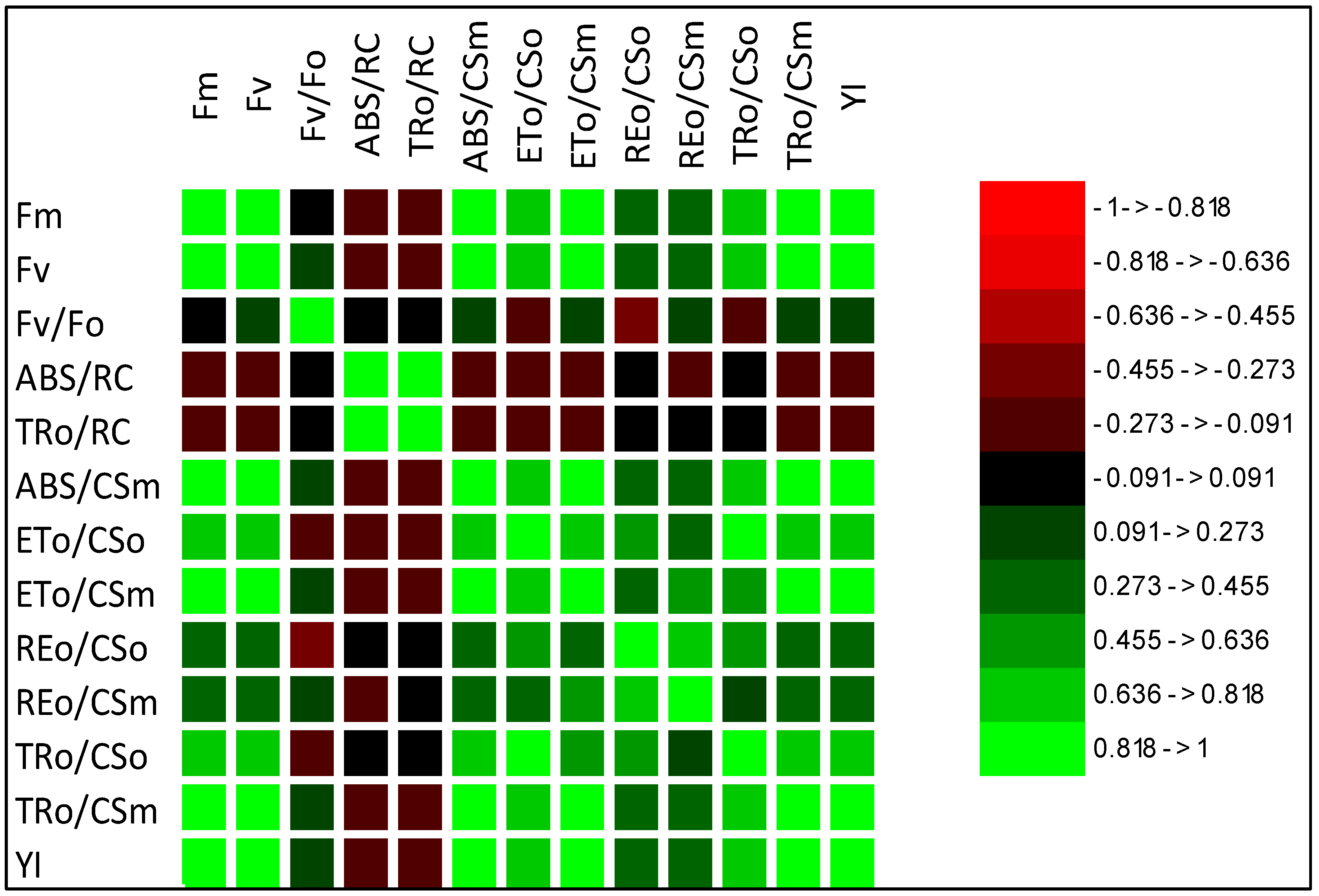
2.1.3. Correlation
2.1.4. Cluster Analysis
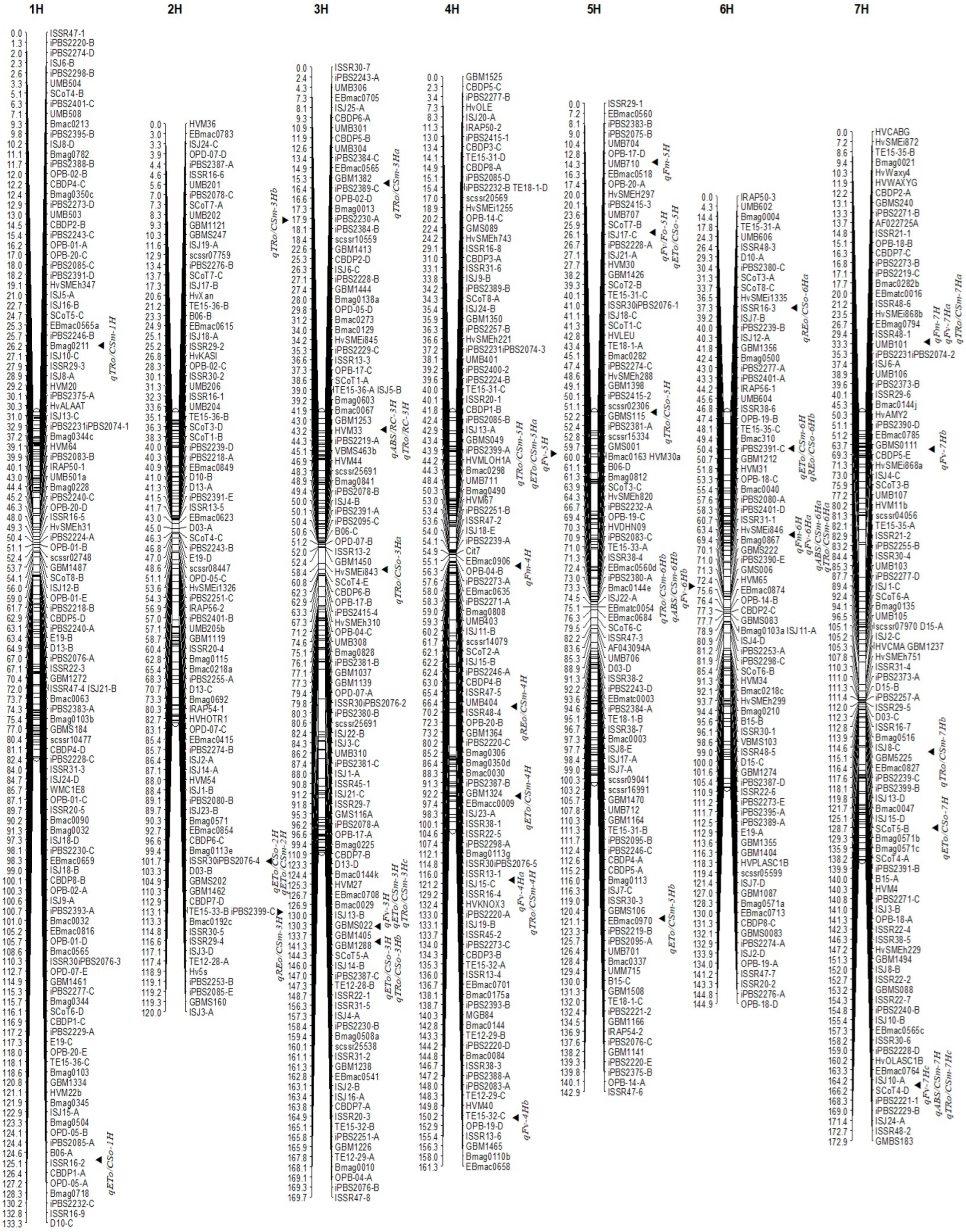
2.2. Linkage Groups
2.3. QTL Mapping
2.3.1. Fm Parameter
2.3.2. Fv Parameter
2.3.3. Fv/Fo Parameter
2.3.4. ABS/RC Parameter
2.3.5. TRo/RC Parameter
2.3.6. ABS/CSm Parameter
2.3.7. ETo/CSo Parameter
2.3.8. ETo/CSm Parameter
2.3.9. REo/CSo Parameter
2.3.10. REo/CSm Parameter
2.3.11. TRo/CSo Parameter
2.3.12. TRo/CSm Parameter
3. Discussion
4. Materials and Methods
4.1. Plant Materials and Experimental Conditions
4.2. Measurement of OJIP Test Parameters
4.3. Statistical Analyses for Phenotypic Data
4.4. Measurement of Genotypic Data
4.5. Preparation of Linkage Map
4.6. Identification of Closely Linked QTLs
5. Conclusions
Supplementary Materials
Author Contributions
Funding
Institutional Review Board Statement
Informed Consent Statement
Data Availability Statement
Acknowledgments
Conflicts of Interest
Abbreviations
| Abbreviation | Definition |
| ROSs | Reactive Oxygen Species |
| PSI and PSII | Photosystem I and II |
| RC | Reaction Center |
| ABA | Abscisic Acid |
| OJIP test | Fast chlorophyll a fluorescence induction |
| Fo and Fm | Minimum and Maximum Fluorescence |
| QA and QB | Quinone A and B (the first and second electron-accepting molecules) |
| ATP | Adenosine Triphosphate |
| NADPH | Nicotinamide Adenine Dinucleotide Phosphate |
| ABS | Absorption flux |
| ET | Electron Transport |
| TR | Trapped energy flux |
| CS | Cross-Section |
| QTLs | Quantitative Trait Loci |
| MTAs | Marker-Trait Associations |
| GWAS | Genome-Wide Association Study |
| MLM | Mixed Linear Model |
| ANOVA | Analysis of Variance |
| MANOVA | Multivariate Analysis of Variance |
| cM | centi-Morgan |
| SSR | Simple Sequence Repeat (Microsatellite) |
| RAPD | Random Amplified Polymorphic DNA |
| ISSR | Inter Simple Sequence Repeat |
| SCoT | Start Codon Target |
| CBDP | CAAT Box-Derived Polymorphism |
| iPBS | inter Primer Binding Site |
| EST | Expressed Sequence Tag |
| IRAP | Inter-Retrotransposon Amplified Polymorphism |
| TE | Transposable Element |
| ISJ | Intron-exon Splice Junctions |
| RILs | Recombinant Inbred Lines |
| SSD | Single Seed Descent |
| SPII | Seed and Plant Improvement Institute |
| ICARDA | International Center for Agricultural Research in the Dry Areas |
| PCR | Polymerase Chain Reaction |
| GCIM | Genome-Wide Composite Interval Mapping |
| LOD | Logarithm of Odd |
| MAS | Marker-Assisted Selection |
References
- Kopecká, R.; Kameniarová, M.; Černý, M.; Brzobohatý, B.; Novák, J. Abiotic stress in crop production. Int. J. Mol. Sci. 2023, 24, 6603. [Google Scholar] [CrossRef] [PubMed]
- Soualiou, S.; Duan, F.; Li, X.; Zhou, W. Crop production under cold stress: An understanding of plant responses, acclimation processes, and management strategies. Plant Physiol. Biochem. 2022, 190, 47–61. [Google Scholar] [CrossRef] [PubMed]
- Shi, Y.; Yang, S. ABA regulation of the cold stress response in plants. In Abscisic Acid: Metabolism, Transport and Signaling; Zhang, D.P., Ed.; Springer: Dordrecht, The Netherlands, 2014; pp. 337–363. [Google Scholar]
- Nishiyama, I. Damage due to extreme temperatures. In Science of the Rice Plant; Matsuo, T., Kumazawa, K., Ishii, R., Ishihara, H., Hirata, H., Eds.; Food and Agriculture Policy Research Center: Tokyo, Japan, 1995; pp. 769–812. [Google Scholar]
- Thakur, P.; Kumar, S.; Malik, J.A.; Berger, J.D.; Nayyar, H. Cold stress effects on reproductive development in grain crops: An overview. Environ. Exp. Bot. 2010, 67, 429–443. [Google Scholar] [CrossRef]
- Zhou, X.; Muhammad, I.; Lan, H.; Xia, C. Recent advances in the analysis of cold tolerance in maize. Front. Plant Sci. 2022, 13, 866034. [Google Scholar] [CrossRef] [PubMed]
- Ren, C.; Kuang, Y.; Lin, Y.; Guo, Y.; Li, H.; Fan, P.; Li, S.; Liang, Z. Overexpression of grape ABA receptor gene VaPYL4 enhances tolerance to multiple abiotic stresses in Arabidopsis. BMC Plant Biol. 2022, 22, 271. [Google Scholar] [CrossRef] [PubMed]
- Adhikari, L.; Baral, R.; Paudel, D.; Min, D.; Makaju, S.O.; Poudel, H.P.; Acharya, J.P.; Missaoui, A.M. Cold stress in plants: Strategies to improve cold tolerance in forage species. Plant Stress 2022, 4, 100081. [Google Scholar] [CrossRef]
- Corsi, S.; Friedrich, T.; Kassam, A.; Pisante, M.; de Moraes Sà, J.C. Soil organic carbon accumulation and greenhouse gas emission reductions from conservation agriculture: A literature review. In Integrated Crop Management; AGP/FAO: Rome, Italy, 2012; p. 101. [Google Scholar]
- Muñoz-Amatriaín, M.; Hernandez, J.; Herb, D.; Baenziger, P.S.; Bochard, A.M.; Capettini, F.; Casas, A.; Cuesta-Marcos, A.; Einfeldt, C.; Fisk, S.; et al. Perspectives on low temperature tolerance and vernalization sensitivity in barley: Prospects for facultative growth habit. Front. Plant Sci. 2020, 11, 585927. [Google Scholar] [CrossRef]
- Sallam, A.H.; Smith, K.P.; Hu, G.; Sherman, J.; Baenziger, P.S.; Wiersma, J.; Duley, C.; Stockinger, E.J.; Sorrells, M.E.; Szinyei, T.; et al. Cold conditioned: Discovery of novel alleles for low-temperature tolerance in the Vavilov barley collection. Front. Plant Sci. 2021, 12, 800284. [Google Scholar] [CrossRef]
- Tondelli, A.; Pagani, D.; Naseh Ghafoori, I.; Rahimi, M.; Ataei, R.; Rizza, F.; Flavell, A.J.; Cattivelli, L. Allelic variation at Fr-H1/Vrn-H1 and Fr-H2 loci is the main determinant of frost tolerance in spring barley. Environ. Exp. Bot. 2014, 106, 148–155. [Google Scholar] [CrossRef]
- Marè, C.; Mazzucotelli, E.; Crosatti, C.; Francia, E.; Stanca, A.; Cattivelli, L. Hv-WRKY38: A new transcription factor involved in cold- and drought-response in barley. Plant Mol. Biol. 2004, 55, 399–416. [Google Scholar] [CrossRef]
- Skinner, J.S.; von Zitzewitz, J.; Szucs, P.; Marquez-Cedillo, L.; Filichkin, T.; Amundsen, K.; Stockinger, E.J.; Thomashow, M.F.; Chen, T.H.; Hayes, P.M. Structural, functional, and phylogenetic characterization of a large CBF gene family in barley. Plant Mol. Biol. 2005, 59, 533–551. [Google Scholar] [CrossRef] [PubMed]
- Jeknić, Z.; Pillman, K.A.; Dhillon, T.; Skinner, J.S.; Veisz, O.; Cuesta-Marcos, A.; Hayes, P.M.; Jacobs, A.K.; Chen, T.H.; Stockinger, E.J. Hv-CBF2A overexpression in barley accelerates COR gene transcript accumulation and acquisition of freezing tolerance during cold acclimation. Plant Mol. Biol. 2014, 84, 67–82. [Google Scholar] [CrossRef] [PubMed]
- Choi, D.W.; Rodriguez, E.M.; Close, T.J. Barley Cbf3 gene identification, expression pattern, and map location. Plant Physiol. 2002, 129, 1781–1787. [Google Scholar] [CrossRef] [PubMed]
- Hackenberg, M.; Gustafson, P.; Langridge, P.; Shi, B.J. Differential expression of microRNAs and other small RNAs in barley between water and drought conditions. Plant Biotechnol. J. 2015, 13, 2–13. [Google Scholar] [CrossRef]
- Megha, S.; Basu, U.; Kav, N.N.V. Regulation of low temperature stress in plants by microRNAs. Plant Cell Environ. 2018, 41, 1–15. [Google Scholar] [CrossRef]
- Andrews, J.R.; Fryer, M.J.; Baker, N.R. Characterization of chilling effects on photosynthetic performance of maize crops during early season growth using chlorophyll fluorescence. J. Exp. Bot. 1995, 46, 1195–1203. [Google Scholar] [CrossRef]
- Li, X.; Cai, J.; Liu, F.; Zhou, Q.; Li, X.; Cao, W.; Jiang, D. Wheat plants exposed to winter warming are more susceptible to low temperature stress in the spring. Plant Growth Regul. 2015, 77, 11–19. [Google Scholar] [CrossRef]
- Maxwell, K.; Johnson, G. Chlorophyll fluorescence a practical guide. J. Exp. Bot. 2000, 51, 659–668. [Google Scholar] [CrossRef]
- Apostolova, E.L.; Dobrikova, A.G.; Ivanova, P.I.; Petkanchin, I.B.; Taneva, S.G. Relationship between the organization of the PS II super complex and the functions of the photosynthetic apparatus. J. Photochem. Photobiol. B Biol. 2006, 83, 114–122. [Google Scholar] [CrossRef]
- Yuan, W.; Suo, J.; Shi, B.; Zhou, C.; Bai, B.; Bian, H.; Zhu, M.; Han, N. The barley MiR393has multiple roles in regulation of seedling growth, stomatal density, and drought stress tolerance. Plant Physiol. Biochem. 2019, 142, 303–311. [Google Scholar] [CrossRef]
- Kalaji, H.M.; Jajoo, A.; Oukarroum, A.; Brestic, M.; Zivcak, M.; Samborska, I.A.; Center, M.D.; Łukasik, I.; Goltsev, V.; Ladle, R.J. Chlorophyll a fluorescence as a tool to monitor physiological status of plants under abiotic stress conditions. Acta Physiol. Plant 2016, 38, 102. [Google Scholar] [CrossRef]
- Baker, N.R. Chlorophyll fluorescence: A probe of photosynthesis in vivo. Annu. Rev. Plant Biol. 2008, 59, 89–113. [Google Scholar] [CrossRef] [PubMed]
- Lazár, D.; Pospísil, P.; Naus, J. Decrease of fluorescence intensity after the K step in chlorophyll a fluorescence induction is suppressed by electron acceptors and donors to photosystem 2. Photosynthetica 1999, 37, 255–265. [Google Scholar] [CrossRef]
- Strasser, R.J.; Srivastava, A.; Tsimilli-Michael, M. The fluorescence transient as a tool to characterize and screen photosynthetic samples. In Probing Photosynthesis: Mechanism, Regulation and Adaptation; Yunus, M., Pathre, U., Mohanty, P., Eds.; Taylor and Francis: Oxford, UK; CRC Press: Boca Raton, FL, USA, 2000; pp. 445–483. [Google Scholar]
- Kautsky, H.; Hirsch, A. Neue versuche zur kohlensäureassimilation. Naturwissenschaften 1931, 19, 964. [Google Scholar] [CrossRef]
- Strasser, R.J.; Tsimilli-Michael, M.; Srivastava, A. Analysis of the chlorophyll a fluorescence transient. In Chlorophyll a Fluorescence. Advances in Photosynthesis and Respiration; Papageorgiou, G.C., Govindjee, Eds.; Springer: Dordrecht, The Netherlands, 2004; pp. 322–362. [Google Scholar]
- Misra, A.N.; Misra, M.; Singh, R. Chlorophyll fluorescence in plant biology. In Biophysics; Misra, A.N., Ed.; Intech Europe: Rijeka, Croatia, 2012; pp. 171–192. [Google Scholar]
- Makhtoum, S.; Sabouri, H.; Gholizadeh, A.; Ahangar, L.; Katouzi, M.; Mastinu, A. Genomics and physiology of chlorophyll fluorescence parameters in Hordeum vulgare L. under drought and salt stresses. Plants 2023, 12, 3515. [Google Scholar] [CrossRef] [PubMed]
- Sabouri, H.; Taliei, F.; Kazerani, B.; Ghasemi, S.; Katouzi, M. Identification of novel and stable genomic regions associated with barley resistance to spot form net blotch disease under different temperature conditions during the reproductive stage. Plant Pathol. 2023, 72, 951–963. [Google Scholar] [CrossRef]
- Taliei, F.; Sabouri, H.; Kazerani, B.; Ghasemi, S. Finding stable and closely linked QTLs against spot blotch in different planting dates during the adult stage in barley. Sci. Rep. 2024, 14, 818. [Google Scholar] [CrossRef]
- Sabouri, H.; Kazerani, B.; Fallahi, H.A.; Dehghan, M.A.; Mohammad Alegh, S.; Dadras, A.R.; Katouzi, M.; Mastinu, A. Association analysis of yellow rust, fusarium head blight, tan spot, powdery mildew and brown rust horizontal resistance genes in wheat. Physiol. Mol. Plant Pathol. 2022, 118, 101808. [Google Scholar] [CrossRef]
- Elakhdar, A.; Slaski, J.J.; Kubo, T.; Hamwieh, A.; Ramirez, G.H.; Beattie, A.D.; Capo-chichi, L.J.A. Genome-wide association analysis provides insights into the genetic basic of photosynthetic responses to low-temperature stress in spring barley. Front. Plant Sci. 2023, 14, 1159016. [Google Scholar] [CrossRef]
- Rieseberg, L.; Archer, M.; Wayne, R. Transgressive segregation, adaptation and speciation. Heredity 1999, 83, 363–372. [Google Scholar] [CrossRef]
- Mackay, I.J.; Cockram, J.; Howell, P.; Powell, W. Understanding the classics: The unifying concepts of transgressive segregation, inbreeding depression and heterosis and their central relevance for crop breeding. Plant Biotechnol. J. 2021, 19, 26–34. [Google Scholar] [CrossRef]
- Fernandez Martinez, J.; Dominguez Gimenez, J.; Jimenez, A.; Hernandez, L. Use of the single seed descent method in breeding safflower (Carthamus tinctorius L.). Plant Breed. 1986, 97, 364–367. [Google Scholar] [CrossRef]
- Miura, K.; Tada, Y. Regulation of water, salinity, and cold stress responses by salicylic acid. Front. Plant Sci. 2014, 5, 1–12. [Google Scholar] [CrossRef] [PubMed]
- Chaves, M.M.; Flexas, J.; Pinheiro, C. Photosynthesis under drought and salt stress: Regulation mechanisms from whole plant to cell. Ann. Bot. 2009, 103, 551–560. [Google Scholar] [CrossRef] [PubMed]
- Lotfi, R.; Kalaji, H.M.; Valizadeh, G.R.; Khalilvand Behrozyar, E.; Hemati, A.; Gharavi-Kochebagh, P.; Ghassemi, A. Effects of humic acid on photosynthetic efficiency of rapeseed plants growing under different watering conditions. Photosynthetica 2018, 56, 962–970. [Google Scholar] [CrossRef]
- Falconer, D.S.; Mackay, T.F.C. Introduction to Quantitative Genetics, 4th ed.; Addison Wesley Longman: Harlow, UK, 1996. [Google Scholar]
- Reif, J.C.; Liu, W.; Gowda, M.; Maurer, H.P.; Möhring, J.; Fischer, S.; Schechert, A.; Würschum, T. Genetic basis of agronomically important traits in sugar beet (Beta vulgaris L.) investigated with joint linkage association mapping. Theor. Appl. Genet. 2010, 121, 1489–1499. [Google Scholar] [CrossRef]
- Remington, D.L.; Ungerer, M.C.; Purugganan, M.D. Map-based cloning of quantitative trait loci: Progress and prospects. Genet. Res. 2001, 78, 213–218. [Google Scholar] [CrossRef]
- Tanksley, S.D.; Ganal, M.W.; Martin, G.B. Chromosome landing: A paradigm for map-based gene cloning in plants with large genomes. Trends Genet. 1995, 11, 63–68. [Google Scholar] [CrossRef] [PubMed]
- Wing, R.A.; Zhang, H.B.; Tanksley, S.D. Map-based cloning in crop plants. Tomato as a model system: I. Genetic and physical mapping of jointless. Mol. Genet. Genom. 1994, 242, 681–688. [Google Scholar] [CrossRef]
- Godwin, I.D.; Rutkoski, J.; Varshney, R.K.; Hickey, L.T. Technological perspectives for plant breeding. Theor. Appl. Genet. 2019, 132, 555–557. [Google Scholar] [CrossRef]
- Collard, B.C.Y.; Jahufer, M.Z.Z.; Brouwer, J.B.; Pang, E.C.K. An introduction to markers, quantitative trait loci (QTL) mapping and marker-assisted selection for crop improvement: The basic concepts. Euphytica 2005, 142, 169–196. [Google Scholar] [CrossRef]
- Powell, W.; Caligari, P.D.S.; Thomas, W.T.B. Comparison of spring barley lines produced by single seed descent, pedigree inbreeding and doubled haploidy. Plant Breed. 1986, 97, 138–146. [Google Scholar] [CrossRef]
- Yang, C.; Yang, H.; Xu, Q.; Wang, Y.; Sang, Z.; Yuan, H. Comparative metabolomics analysis of the response to cold stress of resistant and susceptible Tibetan hulless barley (Hordeum distichon). Phytochemistry 2020, 174, 112346. [Google Scholar] [CrossRef]
- Otero, E.A.; Miralles, D.J.; Benech-Arnold, R.L. Development of a precise thermal time model for grain filling in barley: A critical assessment of base temperature estimation methods from field-collected data. Field Crop. Res. 2021, 260, 108003. [Google Scholar] [CrossRef]
- Zadoks, J.C.; Chang, T.T.; Konzak, C.F. A decimal code for the growth stages of cereals. Weed Res. 1974, 14, 415–421. [Google Scholar] [CrossRef]
- Rapacz, M.; Wójcik-Jagla, M.; Fiust, A.; Kalaji, H.M.; Kościelniak, J. Genome-wide association of chlorophyll fluorescence OJIP transient parameters connected with soil drought response in barley. Front. Plant Sci. 2019, 10, 78. [Google Scholar] [CrossRef] [PubMed]
- Janeeshma, E.; Johnson, R.; Amritha, M.S.; Noble, L.; Aswathi, K.P.R.; Telesiński, A.; Kalaji, H.M.; Auriga, A.; Puthur, J.T. Modulations in chlorophyll a fluorescence based on intensity and spectral variations of light. Int. J. Mol. Sci. 2022, 23, 5599. [Google Scholar] [CrossRef] [PubMed]
- Stefanov, M.A.; Rashkov, G.D.; Apostolova, E.L. Assessment of the photosynthetic apparatus functions by chlorophyll fluorescence and P700 absorbance in C3 and C4 plants under physiological conditions and under salt stress. Int. J. Mol. Sci. 2022, 23, 3768. [Google Scholar] [CrossRef] [PubMed]
- Li, X.; Meng, X.; Yang, X.; Duan, D. Characterization of chlorophyll fluorescence and antioxidant defense parameters of two Gracilariopsis lemaneiformis strains under different temperatures. Plants 2023, 12, 1670. [Google Scholar] [CrossRef]
- Doyle, J.J.; Doyle, J.L. Isolation of plant DNA from fresh tissue. Focus 1990, 12, 13–15. [Google Scholar]
- Grain Genes (A Database for Triticeae and Avena). Available online: https://wheat.pw.usda.gov/GG3/ (accessed on 24 January 2024).
- An, Z.W.; Xie, L.L.; Cheng, H.; Zhou, Y.; Zhang, Q.; He, X.G.; Huang, H.S. A silver staining procedure for nucleic acids in polyacrylamide gels without fixation and pretreatment. Anal. Biochem. 2009, 391, 77–79. [Google Scholar] [CrossRef] [PubMed]
- Manly, K.F.; Cudmore Jr, R.H.; Meer, J.M. Map Manager QTX, cross-platform software for genetic mapping. Mamm. Genome. 2001, 12, 930–932. [Google Scholar] [CrossRef] [PubMed]
- Kosambi, D.D. The estimation of map distances from recombination values. Ann. Eugen. 1943, 12, 172–175. [Google Scholar] [CrossRef]
- Zhang, Y.W.; Wen, Y.J.; Dunwell, J.M.; Zhang, Y.M. QTL.gCIMapping.GUI v2.0: An R software for detecting small-effect and linked QTLs for quantitative traits in bi-parental segregation populations. Comput. Struct. Biotechnol. J. 2020, 18, 59–65. [Google Scholar] [CrossRef] [PubMed]
- Churchill, G.A.; Doerge, R.W. Empirical threshold values for quantitative trait mapping. Genetics 1994, 138, 963–971. [Google Scholar] [CrossRef]


| OJIP Test Parameters | Years | Badia | Kavir | Min. | Max. | Q1 | Q2 | Q3 | Mean | SEM | Skewness | Kurtosis |
|---|---|---|---|---|---|---|---|---|---|---|---|---|
| Fm | 2018/2019 | 495 | 559 | 484 | 570 | 511.5 | 536 | 550.5 | 531.01 | 2.31 | −0.19 | −1.11 |
| 2019/2020 | 498 | 557 | 488 | 570 | 508.50 | 528 | 547 | 528.27 | 2.22 | 0.08 | −1.15 | |
| 2020/2021 | 396 | 521 | 389 | 533 | 418 | 442 | 471.50 | 447.71 | 3.38 | 0.45 | −0.73 | |
| Fv | 2018/2019 | 416 | 476 | 409 | 485 | 425 | 449 | 467.5 | 447.26 | 2.26 | −0.05 | −1.25 |
| 2019/2020 | 423 | 474 | 416 | 485 | 435.50 | 449 | 469.50 | 451.01 | 2.00 | −0.02 | −1.14 | |
| 2020/2021 | 342 | 439 | 331 | 450 | 349.50 | 370 | 399.50 | 375.23 | 3.06 | 0.63 | −0.53 | |
| Fv/Fo | 2018/2019 | 4.15 | 8.84 | 4.08 | 8.90 | 6.10 | 6.92 | 7.97 | 6.92 | 0.12 | −0.25 | −0.79 |
| 2019/2020 | 4.55 | 8.82 | 4.48 | 8.90 | 6.35 | 7.11 | 7.99 | 7.11 | 0.10 | −0.27 | −0.68 | |
| 2020/2021 | 4.22 | 5.86 | 4.16 | 5.99 | 4.84 | 5.03 | 5.23 | 5.04 | 0.03 | 0.18 | 0.30 | |
| ABS/RC | 2018/2019 | 1.29 | 0.35 | 0.29 | 1.37 | 0.56 | 0.80 | 1.04 | 0.81 | 0.03 | 0.09 | −1.05 |
| 2019/2020 | 1.21 | 0.37 | 0.30 | 1.30 | 0.52 | 0.71 | 0.91 | 0.74 | 0.03 | 0.36 | −0.80 | |
| 2020/2021 | 1.02 | 0.64 | 0.57 | 1.09 | 0.77 | 0.84 | 0.90 | 0.84 | 0.01 | 0.01 | −0.22 | |
| TRo/RC | 2018/2019 | 0.31 | 0.95 | 0.26 | 1.10 | 0.44 | 0.63 | 0.83 | 0.65 | 0.02 | 0.20 | −1.05 |
| 2019/2020 | 0.28 | 0.93 | 0.23 | 1.10 | 0.44 | 0.63 | 0.82 | 0.64 | 0.02 | 0.14 | −0.98 | |
| 2020/2021 | 0.53 | 0.86 | 0.48 | 0.91 | 0.64 | 0.70 | 0.75 | 0.70 | 0.01 | −0.04 | −0.16 | |
| ABS/CSm | 2018/2019 | 485 | 564 | 479 | 570 | 503.5 | 523 | 542 | 523.57 | 2.50 | 0.17 | −1.09 |
| 2019/2020 | 484 | 563 | 478 | 570 | 503 | 529 | 551 | 526.47 | 2.58 | −0.07 | −1.27 | |
| 2020/2021 | 396 | 525 | 389 | 533 | 418 | 442 | 471.50 | 447.71 | 3.38 | 0.45 | −0.73 | |
| ETo/CSo | 2018/2019 | 49.45 | 66.12 | 47.44 | 70.53 | 60.08 | 63.43 | 67.13 | 63.10 | 0.52 | −0.74 | 0.01 |
| 2019/2020 | 50.73 | 65.33 | 47.44 | 70.53 | 60.08 | 63.43 | 67.13 | 63.10 | 0.52 | −0.74 | 0.01 | |
| 2020/2021 | 49.21 | 62.14 | 46.27 | 66.01 | 52.91 | 56.80 | 59.97 | 56.80 | 0.45 | 0.04 | −0.76 | |
| ETo/CSm | 2018/2019 | 363 | 411 | 355 | 416 | 377 | 390 | 404 | 390.69 | 1.65 | −0.08 | −1.07 |
| 2019/2020 | 359 | 410 | 350 | 416 | 375.50 | 385 | 402 | 386.54 | 1.67 | −0.04 | −0.88 | |
| 2020/2021 | 291 | 398 | 284 | 404 | 316 | 335 | 364 | 340.96 | 2.83 | 0.33 | −0.89 | |
| REo/CSo | 2018/2019 | 29.34 | 47.16 | 27.69 | 50.64 | 41.44 | 45.37 | 48.44 | 44.24 | 0.55 | −1.07 | 0.40 |
| 2019/2020 | 32.76 | 47.38 | 29.57 | 50.62 | 41.21 | 45.15 | 48.20 | 44.13 | 0.52 | −1.02 | 0.31 | |
| 2020/2021 | 33.91 | 41.88 | 30.40 | 45.98 | 37.10 | 39.30 | 41.84 | 39.23 | 0.35 | −0.45 | −0.43 | |
| REo/CSm | 2018/2019 | 196 | 291 | 188 | 300 | 259 | 273 | 288 | 269.45 | 2.58 | −1.43 | 1.99 |
| 2019/2020 | 199 | 290 | 190 | 300 | 265 | 276 | 291.50 | 272.95 | 2.44 | −1.67 | 2.85 | |
| 2020/2021 | 191 | 285 | 182 | 287 | 222.50 | 237.39 | 252 | 237.39 | 2.10 | 0.03 | −0.15 | |
| TRo/CSo | 2018/2019 | 59.56 | 74.83 | 55.87 | 77.65 | 66.01 | 70.42 | 74.33 | 69.67 | 0.55 | −0.63 | −0.67 |
| 2019/2020 | 60.43 | 73.99 | 55.06 | 77.64 | 64.59 | 70.43 | 74.76 | 69.37 | 0.60 | −0.48 | −0.89 | |
| 2020/2021 | 58.19 | 70.48 | 53.25 | 75.69 | 58.74 | 62.90 | 66.84 | 62.91 | 0.53 | 0.30 | −0.75 | |
| TRo/CSm | 2018/2019 | 419 | 479 | 412 | 485 | 429 | 446 | 466 | 447.66 | 2.10 | 0.17 | −1.08 |
| 2019/2020 | 423 | 477 | 415 | 485 | 433 | 457 | 472 | 452.11 | 2.14 | −0.23 | −1.27 | |
| 2020/2021 | 340 | 441 | 331 | 450 | 349.50 | 370 | 399.50 | 375.32 | 3.08 | 0.64 | −0.52 |
| OJIP Test Parameters | Years | QTL | Chr. | Pos. (cM) | LOD | Flanking Markers | Ϭg2 | R2 (%) | AE a | DPE b |
|---|---|---|---|---|---|---|---|---|---|---|
| Fm | 2018/2019 | qFm-6H | 6H | 67.65 | 9.97 | HvSMEi846-Bmag0867 | 151.66 | 14.09 | 12.32 | Kavir |
| qFm-7H | 7H | 33.25 | 2.93 | UMB101 | 30.51 | 2.83 | 5.52 | Kavir | ||
| 2019/2020 | qFm-4H | 4H | 55.70 | 4.14 | EBmac0906-OPB-04-B | 37.03 | 6.93 | 6.09 | Kavir | |
| qFm-5H | 5H | 13.56 | 6.57 | OPB-17-D-UMB710 | 57.85 | 10.82 | 7.61 | Kavir | ||
| qFm-6H | 6H | 67.65 | 3.60 | HvSMEi846-Bmag0867 | 26.82 | 10.01 | 5.18 | Kavir | ||
| qFm-7H | 7H | 33.25 | 8.44 | UMB101 | 42.89 | 8.02 | 6.55 | Kavir | ||
| 2020/2021 | qFm-4H | 4H | 55.70 | 6.24 | EBmac0906-OPB-04-B | 308.84 | 8.91 | 17.57 | Kavir | |
| qFm-5H | 5H | 13.56 | 8.48 | OPB-17-D-UMB710 | 315.11 | 10.09 | 17.75 | Kavir | ||
| Fv | 2018/2019 | qFv-3H | 3H | 130.25 | 4.98 | GBMS022 | 14.84 | 2.82 | 3.85 | Kavir |
| qFv-4Ha | 4H | 117.75 | 7.13 | ISSR13-1-ISJ15-C | 33.55 | 6.37 | 5.79 | Kavir | ||
| qFv-4Hb | 4H | 151.10 | 4.06 | ET15-32-C-OPB-19-D | 10.56 | 2.01 | 3.25 | Kavir | ||
| qFv-5H | 5H | 59.98 | 2.63 | Bmac0163 | 7.14 | 1.36 | 2.67 | Kavir | ||
| qFv-6Ha | 6H | 65.94 | 7.12 | HvSMEi846-Bmag0867 | 30.67 | 5.83 | 5.54 | Kavir | ||
| qFv-6Hb | 6H | 74.81 | 6.52 | HVM65-EBmac0874 | 22.74 | 4.32 | 4.77 | Kavir | ||
| qFv-7Hb | 7H | 63.72 | 6.69 | GBMS0111 | 13.46 | 2.56 | −3.67 | Badia | ||
| 2019/2020 | qFv-3H | 3H | 130.25 | 8.33 | GBMS022 | 31.58 | 4.91 | 5.62 | Kavir | |
| qFv-4Ha | 4H | 117.75 | 3.79 | ISSR13-1-ISJ15-C | 30.07 | 4.67 | 5.48 | Kavir | ||
| qFv-5H | 5H | 59.98 | 5.75 | Bmac0163 | 23.75 | 3.69 | 4.87 | Kavir | ||
| qFv-6Ha | 6H | 65.94 | 5.94 | HvSMEi846-Bmag0867 | 44.08 | 6.85 | 6.64 | Kavir | ||
| qFv-7Ha | 7H | 33.25 | 6.68 | UMB101 | 18.27 | 2.84 | 4.27 | Kavir | ||
| qFv-7Hb | 7H | 63.72 | 3.58 | GBMS0111 | 12.86 | 2.00 | −3.59 | Badia | ||
| qFv-7Hc | 7H | 165.22 | 3.37 | ISJ10-A-SCoT4-D | 28.41 | 4.42 | −5.33 | Badia | ||
| 2020/2021 | qFv-4Hb | 4H | 151.10 | 2.78 | ET15-32-C-OPB-19-D | 29.11 | 1.31 | 5.40 | Kavir | |
| qFv-6Ha | 6H | 66.79 | 4.30 | HvSMEi846-Bmag0867 | 157.75 | 7.08 | 12.56 | Kavir | ||
| qFv-6Hb | 6H | 74.81 | 6.17 | HVM65-EBmac0874 | 112.45 | 5.05 | 10.60 | Kavir | ||
| qFv-7Ha | 7H | 33.25 | 7.12 | UMB101 | 106.53 | 4.78 | 10.32 | Kavir | ||
| qFv-7Hb | 7H | 63.72 | 2.67 | GBMS0111 | 41.60 | 1.87 | −6.45 | Badia | ||
| qFv-7Hc | 7H | 165.22 | 4.51 | ISJ10-A-SCoT4-D | 67.09 | 3.01 | −8.19 | Badia | ||
| Fv/Fo | 2018/2019 | qFv/Fo-5H | 5H | 26.08 | 4.84 | ISJ17-C | 0.38 | 19.98 | −0.62 | Badia |
| 2019/2020 | qFv/Fo-5H | 5H | 26.08 | 4.73 | ISJ17-C | 0.32 | 19.57 | −0.57 | Badia | |
| 2020/2021 | qFv/Fo-5H | 5H | 26.08 | 2.84 | ISJ17-C | 0.04 | 12.27 | −0.19 | Badia | |
| ABS/RC | 2018/2019 | qABS/RC-3H | 3H | 43.21 | 3.04 | HVM33 | 0.01 | 12.77 | −0.11 | Kavir |
| 2019/2020 | qABS/RC-3H | 3H | 43.21 | 4.17 | HVM33 | 0.01 | 13.10 | −0.10 | Kavir | |
| 2020/2021 | qABS/RC-3H | 3H | 43.21 | 2.67 | HVM33 | 0.01 | 11.31 | −0.05 | Kavir | |
| TRo/RC | 2018/2019 | qTRo/RC-3H | 3H | 43.21 | 2.69 | HVM33 | 0.07 | 11.40 | −0.08 | Badia |
| 2020/2021 | qTRo/RC-3H | 3H | 43.21 | 3.30 | HVM33 | 0.01 | 10.61 | −0.04 | Badia | |
| ABS/CSm | 2018/2019 | qABS/CSm-6Ha | 6H | 67.65 | 5.83 | HvSMEi846-Bmag0867 | 82.60 | 7.91 | 9.09 | Kavir |
| qABS/CSm-7H | 7H | 165.22 | 6.78 | ISJ10-A-SCoT4-D | 89.98 | 8.62 | −9.49 | Badia | ||
| 2019/2020 | qABS/CSm-6Ha | 6H | 67.65 | 11.23 | HvSMEi846-Bmag0867 | 103.87 | 8.19 | 10.19 | Kavir | |
| qABS/CSm-6Hb | 6H | 74.81 | 5.52 | HVM65-EBmac0874 | 33.88 | 2.67 | 5.82 | Kavir | ||
| qABS/CSm-7H | 7H | 165.22 | 2.89 | ISJ10-A-SCoT4-D | 22.37 | 1.76 | −4.73 | Badia | ||
| 2020/2021 | qABS/CSm-6Hb | 6H | 74.81 | 2.85 | HVM65-EBmac0874 | 98.87 | 2.85 | 9.94 | Kavir | |
| ETo/CSo | 2018/2019 | qETo/CSo-1H | 1H | 125.07 | 4.32 | ISSR16-2 | 7.89 | 7.26 | 2.81 | Kavir |
| qETo/CSo-2H | 2H | 101.71 | 3.13 | ISSR30iPBS2076-4 | 5.30 | 4.88 | 2.30 | Kavir | ||
| qETo/CSo-3H | 3H | 139.38 | 5.74 | GBM1405-GBM1288 | 20.32 | 18.69 | −4.51 | Badia | ||
| qETo/CSo-5H | 5H | 26.08 | 3.67 | ISJ17-C | 6.38 | 5.87 | 2.53 | Kavir | ||
| qETo/CSo-7H | 7H | 126.86 | 3.19 | ISJ15-D-SCoT5-B | 9.29 | 8.55 | 3.05 | Kavir | ||
| 2019/2020 | qETo/CSo-1H | 1H | 125.07 | 4.32 | ISSR16-2 | 7.89 | 7.26 | 2.81 | Kavir | |
| qETo/CSo-2H | 2H | 101.71 | 3.13 | ISSR30iPBS2076-4 | 5.30 | 4.88 | 2.30 | Kavir | ||
| qETo/CSo-3H | 3H | 139.38 | 5.74 | GBM1405-GBM1288 | 20.32 | 18.69 | −4.51 | Badia | ||
| qETo/CSo-5H | 5H | 26.08 | 3.67 | ISJ17-C | 6.38 | 5.87 | 2.53 | Kavir | ||
| qETo/CSo-7H | 7H | 126.86 | 3.19 | ISJ15-D-SCoT5-B | 9.29 | 8.55 | 3.05 | Kavir | ||
| 2020/2021 | qETo/CSo-1H | 1H | 125.07 | 3.12 | ISSR16-2 | 2.19 | 3.64 | 1.48 | Kavir | |
| qETo/CSo-3H | 3H | 139.38 | 5.74 | GBM1405-GBM1288 | 6.92 | 11.51 | −2.63 | Badia | ||
| qETo/CSo-5H | 5H | 26.08 | 5.46 | ISJ17-C | 3.41 | 5.67 | 1.85 | Kavir | ||
| qETo/CSo-7H | 7H | 126.86 | 3.09 | ISJ15-D-SCoT5-B | 1.97 | 3.27 | 1.40 | Kavir | ||
| ETo/CSm | 2018/2019 | qETo/CSm-2H | 2H | 101.71 | 2.88 | ISSR30iPBS2076-4 | 14.53 | 4.31 | 3.81 | Kavir |
| qETo/CSm-3H | 3H | 130.25 | 4.22 | GBMS022 | 26.77 | 7.94 | 5.17 | Kavir | ||
| qETo/CSm-4H | 4H | 93.90 | 3.45 | GBM1324-EBmacc0009 | 39.90 | 11.84 | 6.32 | Kavir | ||
| qETo/CSm-5Ha | 5H | 59.98 | 2.96 | Bmac0163 | 18.73 | 10.56 | 4.33 | Kavir | ||
| qETo/CSm-5Hb | 5H | 121.08 | 3.65 | EBmac0970 | 21.93 | 6.50 | 4.68 | Kavir | ||
| qETo/CSm-6H | 6H | 50.37 | 4.03 | iPBS2391-C | 19.35 | 5.74 | −4.40 | Badia | ||
| 2019/2020 | qETo/CSm-2H | 2H | 101.71 | 4.85 | ISSR30iPBS2076-4 | 28.21 | 8.22 | 5.31 | Kavir | |
| qETo/CSm-4H | 4H | 93.90 | 3.63 | GBM1324-EBmacc0009 | 49.49 | 14.41 | 7.03 | Kavir | ||
| qETo/CSm-5Ha | 5H | 59.98 | 5.16 | Bmac0163 | 37.34 | 10.87 | 6.11 | Kavir | ||
| qETo/CSm-5Hb | 5H | 121.08 | 4.15 | EBmac0970 | 30.38 | 8.85 | 5.51 | Kavir | ||
| qETo/CSm-6H | 6H | 50.37 | 3.79 | iPBS2391-C | 21.94 | 6.39 | −4.68 | Badia | ||
| 2020/2021 | qETo/CSm-3H | 3H | 130.25 | 5.67 | GBMS022 | 77.99 | 7.99 | 8.83 | Kavir | |
| qETo/CSm-4H | 4H | 93.90 | 3.03 | GBM1324-EBmacc0009 | 56.36 | 10.78 | 7.51 | Kavir | ||
| qETo/CSm-5Ha | 5H | 59.98 | 3.97 | Bmac0163 | 54.75 | 10.61 | 7.40 | Kavir | ||
| qETo/CSm-5Hb | 5H | 121.08 | 3.62 | EBmac0970 | 45.19 | 4.63 | 6.72 | Kavir | ||
| qETo/CSm-6H | 6H | 50.37 | 4.78 | iPBS2391-C | 48.17 | 4.94 | −6.94 | Badia | ||
| REo/CSo | 2018/2019 | qREo/CSo-6Ha | 6H | 37.33 | 2.57 | ISSR16-3 | 7.29 | 10.08 | 2.70 | Kavir |
| qREo/CSo-6Hb | 6H | 50.37 | 2.78 | iPBS2391-C | 9.44 | 13.06 | −3.07 | Badia | ||
| 2019/2020 | qREo/CSo-6Ha | 6H | 37.33 | 2.58 | ISSR16-3 | 7.26 | 10.06 | 2.69 | Kavir | |
| qREo/CSo-6Hb | 6H | 50.37 | 2.85 | iPBS2391-C | 9.60 | 13.29 | −3.10 | Badia | ||
| 2020/2021 | qREo/CSo-6Hb | 6H | 50.37 | 3.71 | iPBS2391-C | 3.49 | 14.14 | −1.87 | Badia | |
| REo/CSm | 2018/2019 | qREo/CSm-3H | 3H | 129.98 | 2.75 | ISJ13-B | 204.43 | 12.48 | −14.30 | Badia |
| qREo/CSm-4H | 4H | 66.38 | 3.31 | UMB404 | 197.61 | 12.07 | 14.06 | Kavir | ||
| 2019/2020 | qREo/CSm-3H | 3H | 129.98 | 2.91 | ISJ13-B | 216.57 | 13.24 | −14.72 | Badia | |
| qREo/CSm-4H | 4H | 66.38 | 3.13 | UMB404 | 185.60 | 11.35 | 13.62 | Kavir | ||
| TRo/CSo | 2018/2019 | qTRo/CSo-3Ha | 3H | 56.37 | 2.77 | GBM1450-HvSMEi843 | 6.65 | 10.12 | 2.58 | Kavir |
| qTRo/CSo-3Hb | 3H | 138.43 | 2.98 | GBM1405-GBM1288 | 11.59 | 12.41 | −3.40 | Badia | ||
| qTRo/CSo-5H | 5H | 51.64 | 3.17 | scssr02306-GBMS115 | 6.96 | 10.46 | 2.64 | Kavir | ||
| 2019/2020 | qTRo/CSo-3Ha | 3H | 56.37 | 3.18 | GBM1450-HvSMEi843 | 15.21 | 14.63 | 3.90 | Kavir | |
| qTRo/CSo-5H | 5H | 51.64 | 5.50 | scssr02306-GBMS115 | 12.31 | 11.84 | 3.51 | Kavir | ||
| 2020/2021 | qTRo/CSo-3Hb | 3H | 138.43 | 3.17 | GBM1405-GBM1288 | 6.35 | 10.95 | −2.52 | Badia | |
| qTRo/CSo-5H | 5H | 51.64 | 4.97 | scssr02306-GBMS115 | 5.80 | 10.34 | 2.41 | Kavir | ||
| TRo/CSm | 2018/2019 | qTRo/CSm-1H | 1H | 26.18 | 3.87 | Bmag0211 | 8.30 | 1.26 | 2.88 | Kavir |
| qTRo/CSm-3Ha | 3H | 15.88 | 3.94 | GBM1382-iPBS2389-C | 16.67 | 2.54 | 4.08 | Kavir | ||
| qTRo/CSm-3Hb | 3H | 17.94 | 4.58 | iPBS2230-A | 17.34 | 2.64 | 4.16 | Kavir | ||
| qTRo/CSm-3Hc | 3H | 130.25 | 3.52 | GBMS022 | 12.15 | 1.85 | 3.49 | Kavir | ||
| qTRo/CSm-4H | 4H | 117.75 | 2.92 | ISSR13-1-ISJ15-C | 15.55 | 2.37 | 3.94 | Kavir | ||
| qTRo/CSm-5H | 5H | 59.98 | 5.10 | Bmac0163 | 15.50 | 2.36 | 3.94 | Kavir | ||
| qTRo/CSm-6Ha | 6H | 65.94 | 4.01 | HvSMEi846-Bmag0867 | 19.71 | 10.01 | 4.44 | Kavir | ||
| qTRo/CSm-6Hb | 6H | 74.81 | 2.73 | HVM65-EBmac0874 | 9.47 | 1.44 | 3.08 | Kavir | ||
| 2018/2019 | qTRo/CSm-7Ha | 7H | 33.25 | 7.91 | UMB101 | 23.38 | 3.56 | 4.84 | Kavir | |
| qTRo/CSm-7Hb | 7H | 114.55 | 4.35 | ISJ8-C | 9.13 | 1.39 | 3.02 | Kavir | ||
| qTRo/CSm-7Hc | 7H | 165.22 | 8.36 | ISJ10-A-SCoT4-D | 36.67 | 5.59 | −6.06 | Badia | ||
| 2019/2020 | qTRo/CSm-1H | 1H | 26.18 | 5.44 | Bmag0211 | 10.86 | 1.48 | 3.30 | Kavir | |
| qTRo/CSm-3Hb | 3H | 17.94 | 5.37 | iPBS2230-A | 39.47 | 5.39 | 6.28 | Kavir | ||
| qTRo/CSm-3Hc | 3H | 130.25 | 9.81 | GBMS022 | 28.06 | 3.83 | 5.30 | Kavir | ||
| qTRo/CSm-4H | 4H | 117.75 | 4.55 | ISSR13-1-ISJ15-C | 26.11 | 3.57 | 5.11 | Kavir | ||
| qTRo/CSm-5H | 5H | 59.98 | 4.50 | Bmac0163 | 17.52 | 2.40 | 4.19 | Kavir | ||
| qTRo/CSm-6Ha | 6H | 65.94 | 6.70 | HvSMEi846-Bmag0867 | 29.02 | 10.97 | 5.39 | Kavir | ||
| qTRo/CSm-7Ha | 7H | 33.25 | 4.64 | UMB101 | 11.95 | 1.63 | 3.46 | Kavir | ||
| TRo/CSm | 2019/2020 | qTRo/CSm-7Hc | 7H | 165.22 | 3.08 | ISJ10-A-SCoT4-D | 9.85 | 1.35 | −3.14 | Badia |
| 2020/2021 | qTRo/CSm-3Ha | 3H | 15.88 | 5.65 | GBM1382-iPBS2389-C | 105.21 | 7.86 | 10.26 | Kavir | |
| qTRo/CSm-6Ha | 6H | 65.94 | 7.27 | HvSMEi846-Bmag0867 | 171.04 | 12.78 | 13.08 | Kavir | ||
| qTRo/CSm-6Hb | 6H | 74.81 | 5.65 | HVM65-EBmac0874 | 90.58 | 6.77 | 9.52 | Kavir | ||
| qTRo/CSm-7Ha | 7H | 33.25 | 8.45 | UMB101 | 111.19 | 8.31 | 10.54 | Kavir | ||
| qTRo/CSm-7Hb | 7H | 114.55 | 3.34 | ISJ8-C | 44.14 | 3.30 | 6.64 | Kavir | ||
| qTRo/CSm-7Hc | 7H | 165.22 | 3.58 | ISJ10-A-SCoT4-D | 88.27 | 6.59 | −9.40 | Badia |
| OJIP Test Parameters | Description | References |
|---|---|---|
| Fm | The maximal fluorescence level/final step of chlorophyll a fluorescence transient | [54,56] |
| Fv | The maximal variable fluorescence | [54] |
| Fv/Fo | The maximum efficiency of water-splitting complex | [54,55] |
| ABS/RC | Absorption flux per reaction center (RC) corresponding directly to its apparent antenna size | [54,55,56] |
| TRo/RC | Trapping flux leading to quinone A (QA) reduction per RC at t = 0 | [54,55,56] |
| ABS/CSm | Absorption of energy per excited cross-section (CS) approximated by Fm | [54] |
| ETo/CSo | Electron transport flux from QA to quinone B (QB) per CS | [55] |
| ETo/CSm | Electron flux transported by PSII of a photosynthesizing sample CS approximated by Fm | [54] |
| REo/CSo | Electron transport flux until photosystem I (PSI) acceptors per CS | [55] |
| REo/CSm | The flux of electrons from QA to final PSI acceptors per CS of PSII at t = m | [31] |
| TRo/CSo | Maximum trapped exciton flux per CS | [55] |
| TRo/CSm | Excitation energy flux trapped by photosystem II (PSII) of a photosynthesizing sample CS approximated by Fm | [54] |
Disclaimer/Publisher’s Note: The statements, opinions and data contained in all publications are solely those of the individual author(s) and contributor(s) and not of MDPI and/or the editor(s). MDPI and/or the editor(s) disclaim responsibility for any injury to people or property resulting from any ideas, methods, instructions or products referred to in the content. |
© 2024 by the authors. Licensee MDPI, Basel, Switzerland. This article is an open access article distributed under the terms and conditions of the Creative Commons Attribution (CC BY) license (https://creativecommons.org/licenses/by/4.0/).
Share and Cite
Sabouri, H.; Kazerani, B.; Taliei, F.; Ghasemi, S. Genome-Wide Composite Interval Mapping Reveal Closely Linked Quantitative Genes Related to OJIP Test Parameters under Chilling Stress Condition in Barley. Agriculture 2024, 14, 1272. https://doi.org/10.3390/agriculture14081272
Sabouri H, Kazerani B, Taliei F, Ghasemi S. Genome-Wide Composite Interval Mapping Reveal Closely Linked Quantitative Genes Related to OJIP Test Parameters under Chilling Stress Condition in Barley. Agriculture. 2024; 14(8):1272. https://doi.org/10.3390/agriculture14081272
Chicago/Turabian StyleSabouri, Hossein, Borzo Kazerani, Fakhtak Taliei, and Shahram Ghasemi. 2024. "Genome-Wide Composite Interval Mapping Reveal Closely Linked Quantitative Genes Related to OJIP Test Parameters under Chilling Stress Condition in Barley" Agriculture 14, no. 8: 1272. https://doi.org/10.3390/agriculture14081272
APA StyleSabouri, H., Kazerani, B., Taliei, F., & Ghasemi, S. (2024). Genome-Wide Composite Interval Mapping Reveal Closely Linked Quantitative Genes Related to OJIP Test Parameters under Chilling Stress Condition in Barley. Agriculture, 14(8), 1272. https://doi.org/10.3390/agriculture14081272