Modeling Bibb Lettuce Nitrogen Uptake and Biomass Productivity in Vertical Hydroponic Agriculture

Abstract

Global fertilizer production and mismanagement significantly contribute to many harmful environmental impacts, revealing the need for a greater understanding of crop growth and nutrient uptake, which can be used to optimize fertilizer management. This study experimentally adapts first-principles microbial modeling techniques to the hydroponic cultivation of Bibb lettuce (Lactuca sativa) under nitrogen-limited conditions. Monod and Michaelis–Menten’s approaches are applied to predict biomass productivity and nutrient uptake and to evaluate the feasibility of reclaimed wastewater as a nutrient source of nitrogen. Experimental and modeling results reveal significantly different kinetic saturation constants ($K_s$ = 1.331 and $K_m$ = 17.887 mg L⁻¹) and a corresponding cell yield strongly dependent on nutrient concentration, producing visually and compositionally distinct tissue between treatments receiving $\le$26.2 and $\ge$41.7 $\mathrm{m}{\mathrm{g}}_{\mathrm{N}}$ L⁻¹. The resulting Monod model overestimates dry mass predictions during low nutrient conditions, and the collective results support the development of a dynamic Monod curve that is temporally dependent during the plants’ lifecycle. Despite this shortcoming, these results support the feasibility of reclaiming nitrogen from wastewater in hydroponic agriculture, expecting to produce lesser biomass lettuce exhibiting healthy tissue. Furthermore, this study provides a mathematical foundation for agricultural simulations and nutrient management.

1. Introduction

1.1. Fertilizer Shortcomings

During the first quarter of the 21st century, a growing challenge for society is supplying food to an exponentially growing population while preserving agricultural productivity for future generations [1,2,3]. Already, highly urbanized regions have become dependent on tenuous, volatile global food markets to meet their nutritional needs [4]. Meanwhile, the rising price of natural gas, a key input for industrial Haber–Bosch nitrogen processing, has contributed to the rising cost of nitrogen fertilizers. With fertilizer prices up nearly 40% in 2022, nitrogen use efficiency is likely to be a growing concern for commercial growers [5].

Aside from susceptibility to economic perturbation, conventional fertilizer production uses finite resources, chemical components, and energy, making production environmentally unsustainable [6,7,8,9,10,11,12]. Nitrogen-based fertilizers consume 5% of global natural gas demand and are responsible for half of the fossil fuels used in primary food production [13]. Furthermore, farmers often overapply fertilizers to meet production demands and accommodate inefficiencies such as nutrient runoff, which contribute to eutrophication, groundwater contamination, habitat modification, and the production of nitrous oxide (N₂O) with a global warming potential 200–300 times greater than CO₂ [14,15,16,17,18,19,20,21,22,23,24,25]. On the other hand, insufficient fertilization can reduce crop productivity, leading to small, bitter crops with poor nutrient density, resulting in lower profit margins. This dilemma drives the need for research to improve agricultural production and reduce harmful environmental impacts.

1.2. Controlled Environment Agriculture and Wastewater

These concerns have prompted interest in hydroponics and controlled environment agriculture (CEA) to improve the efficiency of conventional field agriculture. While many hydroponic operations use an open-loop flow-through configuration, in which nutrient solution makes a single pass through the crop system before discharge, closed-loop or recirculating hydroponic configurations retain nutrient solution, thereby improving nutrient and water use efficiency [26]. Such systems can potentially utilize nutrient-poor reclaimed wastewater, containing an estimated 40–60 mg L⁻¹ nitrogen, 5–20 mg L⁻¹ phosphorus, and 5–40 mg L⁻¹ potassium [27,28], as either a primary nutrient source or a supplement to offset synthetic fertilizer demand. This could reduce the costs associated with both wastewater treatment and fertilizer production while reducing the negative environmental impacts of discharged wastewater or nutrient-rich hydroponic solutions.

It is also important to understand the presence and role of different forms of these elements (e.g., nitrogen) in wastewater and agriculture. Traditionally-reclaimed wastewater (i.e., aerobic activated sludge) effluent is expected to have nitrogen primarily in the form of nitrate (NO₃⁻), with significantly lesser contributions as nitrite (NO₂⁻) and organic N [29,30,31]. Meanwhile, anaerobically-reclaimed wastewater (i.e., anaerobic membrane bioreactor) effluent can be expected to output nitrogen in the form of ammonium (NH₄⁺) [31]. As expected, studies using this effluent as a nutrient source have determined nitrification is a necessary pre-treatment step for use in hydroponic agriculture [32].

Among these various forms of nitrogen, organic nitrogen covers a diverse range of compounds, from microbial amino acids and proteins to emerging contaminants (e.g., pharmaceuticals, personal care products, caffeine). Some of these emerging contaminants, even in trace concentrations, can accumulate and potentially contribute adverse effects on both crops and consumers [33,34,35] and collectively represent a massive field of current environmental and agronomic research.

Regarding forms of inorganic nitrogen, NH₄⁺ is energetically highly favorable for biomass synthesis due to its reduced oxidation state and is readily assimilated by plant tissues. Agricultural studies show many limited positive and negative effects on lettuce growth, including comparable-to-increased fresh and dry mass, healthy tissue without nutritional disorders, increased root growth, reduced NO₃⁻, P, Mn, Zn, and Cu content in leaves, decreased root zone pH, and decreased maximum NO₃⁻ uptake rates [36,37,38,39]. Conversely, excessive NO₂⁻ concentrations are shown to produce mostly adverse effects on plant color, height, and fresh and dry mass [36]. However, in aerobic environments such as hydroponics, both NH₄⁺ and NO₂⁻ are susceptible to rapid nitrification to NO₃⁻, the primary form of nitrogen in fertilizer for plant uptake. For this reason, this study will focus almost entirely on NO₃⁻.

To create a more sustainable food system for future generations, careful study of plant growth and nutrient uptake is needed to develop mathematical models to support the simulation of plant and nutrient dynamics for various crops. Successful simulation and optimization could allow hydroponic farms to tailor nutritional supply, enabling smart management of productivity, nutrients, water, and waste.

1.3. Modeling in Hydroponics

Through the development of such mathematical models, prior agronomic research has revealed that nutrient uptake and biomass growth are interrelated processes influenced by an organism’s genetics, developmental stages, and environmental conditions, such as nutrients and light exposure [40]. This relationship between an organism and its environment can be modeled by applying ordinary differential equations and metabolic properties encoded as a unique combination of kinetic parameters derived from Michaelis–Menten (MM) enzyme kinetics, which describe nonlinear enzyme-substrate dynamics [41,42,43,44]. Such models have demonstrated that nutrient concentrations, whether in soil or hydroponic solution, positively correlate with nutrient uptake rates up to a saturation point, beyond which additional nutrient supply does not increase uptake [44,45,46].

In the fundamental MM model (Equation (1)), the net uptake rate $U$ of limiting nutrient $i$ is determined by nutrient concentration $S$, maximum uptake rate $U_{max}$, and Michaelis constant $K_m$ which corresponds to nutrient concentration at a half-maximum uptake rate.

$$U^i=U_{ max}^i {\displaystyle \frac{S^i }{K_m^i+S^i}}$$

(1)

The Monod kinetic model is a modification of the MM model traditionally used to describe biomass growth, rather than nutrient uptake, with substrate nutrient concentration (Equation (2)) [47]. These Monod-type kinetic expressions fundamentally assume that biomass growth is implicit in nutrient uptake. The specific growth rate $\mu$ is a function of nutrient concentration $S$, the maximum specific growth rate ${\mu }_{max}$, and the substrate affinity constant $K_s$ [47,48]. This fundamental model does not account for a lag or death phase and focuses only on the growth phase of an organism’s life cycle.

$${\mu }^i={\mu }_{max}^i{\displaystyle \frac{S^i}{K_s^i+S^i}}$$

(2)

While Monod-type kinetics is currently one of the most widely used biokinetic models characterizing microscopic biological phenomena [49], few applications exist for higher-order macroscopic organisms such as plants.

One of the first and most widely referenced examples is the Nitrate Control in Lettuce (NiCoLet) model, which models the growth of lettuce tissue based on the supply of carbon and nitrogen [50,51]. The NiCoLet model pioneered nitrogen kinetics in lettuce; however, experimental research has demonstrated limited accuracy and recurrent issues, including crowding (canopy closure) and significant overestimation of nutrient uptake at high nitrate concentrations [52,53,54]. Meanwhile, in a small series of studies, Silberbush developed a model for the nutrient influx of multiple essential nutrients in hydroponic culture, including $\mathrm{N}{\mathrm{O}}_3^{-}$, $\mathrm{N}{\mathrm{H}}_4^{+}$, ${\mathrm{K}}^{+}$, $\mathrm{P}{\mathrm{O}}_4^{-2}$, $\mathrm{S}{\mathrm{O}}_4^{-2}$, $\mathrm{C}{\mathrm{a}}^{+2}$, $\mathrm{M}{\mathrm{g}}^{+2}$, and $\mathrm{C}{\mathrm{l}}^{-}$ [55,56] as a function of the root surface area. And in another study, Wheeler et al. (1998) modeled uptake in lettuce influenced by nitrate and light intensity over several brief 15–20 min periods during the growth of matured lettuce [46].

1.4. Objectives

This study aims to conduct nitrogen-limited crop cultivation experiments with synthetic nutrient solutions adapted from established literature to generate predictive models for Lactuca sativa (Bibb Lettuce) grown in a vertical hydroponic system. These models pair Michaelis-Menten and Monod kinetics and determine the impact of nitrogen substrate concentration on growth rate, nutrient uptake, and elemental tissue composition. The results are then used to evaluate the feasibility of reclaimed wastewater as a nitrogen source in hydroponic agriculture. Furthermore, it will provide a platform for future nutrient recovery research, cleaner agricultural production and wastewater treatment techniques, and improve agricultural sustainability by reducing harmful environmental impacts.

2. Materials and Methods

2.1. Experimental Configuration

2.1.1. Controlled Environment Chambers

Experiments were conducted in controlled environment chambers, each maintained at 21.5 °C with relative humidity (RH) controlled between 50–70%, with fluctuations due to increasing crop transpiration. Fans circulated airflow within the chamber, and CO₂ concentrations were not controlled. Each chamber was illuminated by twenty 65 W light-emitting diodes (LED) bars (Infinity 2.0 LED; Thrive Agritech, Claymont, DE, USA) positioned 40 cm from the seeding surface and spaced 35 cm apart at the centerline on a 12 h photoperiod. LEDs overhung the edges of the growth area to reduce edge effects (i.e., decreased light intensity on the perimeter). This provided a relatively uniform daily light integral (DLI) blanket of 14.69 ± 0.06 mol m⁻² d⁻¹ (LI-COR LI-1500; Li-Cor., Lincoln, NE, USA), within the optimal range of 14–17 mol m⁻² d⁻¹ for Bibb lettuce [57,58].

2.1.2. Vertical Nutrient Film Technique (NFT) Hydroponic Systems

Environmental chambers were each equipped with six vertical hydroponic systems (2-Tower Farm Wall; ZipGrow, Cornwall, ON, Canada). Each system held two towers containing porous, 3-dimensional fiber webs as support medium (e.g., Matala-type filter), a center strip of felt to wick water and nutrients to the roots, and a drip emitter (Figure 1). Nutrient solution dripped vertically through each tower before being collected in a 5.1 L substrate reservoir and recirculated to the drip emitter manifold via a submerged pump.

Additionally, water withdrawals by evaporation and transpiration were offset by external Auto Top Off (ATO) systems designed in-house. In these ATO systems, deionized water was stored in a reservoir and delivered to hydroponic systems by gravity and regulated by a float valve. This maintained system volume, prevented dehydration, and dampened nutrient concentration fluctuations created by evaporation and transpiration. In future hydroponic operations, not looking to measure and control nutrients precisely, users may benefit more from filling the ATO with dilute nutrient solution rather than purified water.

2.1.3. Seedling Germination and Transplantation

Seeds were planted on the surface divot of 2.5 cm rockwool cubes in a seeding tray, filled halfway with deionized water, covered with a humidity dome, and placed under LEDs for 13 days before transplantation. Seedlings were screened for size by disposing of unsprouted or poorly sprouted seedlings. This mitigated irregular growth during seeding, providing a standardized starting point prior to the introduction of nutrients and the initiation of the exponential growth phase.

Hydroponic towers were manually transplanted with 8 germinated seedlings, spaced evenly, and oriented horizontally as if growing off the wall. Data were recorded throughout the experiments, initializing day 14 after seeding as 0 days after transplantation (DAT) and culminating on 32 DAT.

2.1.4. Treatment Preparation

To determine the effects of soluble nitrogen concentration on specific growth rates, nutrient solution recipes for each treatment were developed with reagent-grade chemicals as determined per Modified Sonneveld’s Solution (MSS) [59] (

Table 1. Nutrient concentrations across treatments.

	Nitrogen Treatment %
	200%	100%	50%	25%	19%	8%
	Macronutrient Concentrations (mg/L)
N	264.47	132.24	66.12	33.06	25.30	10.58
P	*	30.97	*	109.86	93.94	154.05
K	218.42	210.01	*	*	*	*
Ca	*	82.49	*	*	*	*
S	*	32.22	*	*	*	*
Mg	*	24.25	*	*	*	*
Fe	*	1.26	*	*	*	*
	Micronutrient Concentrations (µg/L)
B	*	162.50	*	*	*	*
Mn	*	249.04	*	*	*	*
Zn	*	130.39	*	*	*	*
Cu	*	23.54	*	*	*	*
Mo	*	24.09	*	*	*	*

* Indicates match with MSS baseline concentrations.

).

Each recipe contained different inorganic nitrogen concentrations while aiming to maintain all other nutrients consistent with MSS concentrations. These treatments were determined based on their percentage of inorganic nitrogen relative to the MSS baseline. Upon testing 100% MSS treatment, a range-finding pair of treatments at 50% and 20% are conducted, followed by at least one final round of nitrogen testing at concentrations to approximate the half-velocity constants. These treatments will be referenced by their nitrogen concentration (e.g., 100% MSS baseline as 132 mg L⁻¹).

2.1.5. Controlling pH in Solution

Maintaining pH between 5.5 and 6.5 is ideal for the growth of lettuce in hydroponic systems and poses a challenge when modifying a nutrient solution for experimentation [60]. In regards to pH control, $\mathrm{KOH}$, $\mathrm{KHC}{\mathrm{O}}_3$, and ${\mathrm{H}}_3\mathrm{P}{\mathrm{O}}_4$ are the primary ingredients in hydroponic pH control solutions [61,62]. From this, it may be reasonable to assume that these possess a minimal detrimental impact on crop growth within their utilized concentrations. Additionally, we must consider using paired anions or cations in salts when adjusting for pH. Regardless, nutrients will be measured frequently through experimentation.

Finding suitable cations or anions to match a target pH of 6.0 ± 0.5 posed a challenge with recipe development. Researchers must control the pH within this range while maintaining sufficient concentrations of all 17 macro and micronutrients without overstepping into toxic concentrations and avoiding forming calcium precipitates. Additionally, both sodium and chlorine were avoided to prevent inhibitory effects [63,64]. To overcome this challenge, phosphorus and potassium were utilized in excess as needed. Prior studies demonstrated that a rapid influx of phosphorus can lead to toxicity in lettuce due to its slow response to down-regulate phosphorus uptake [65,66,67]. However, by maintaining elevated concentrations through the entire life cycle, these effects were assumed to be mitigated.

2.1.6. Stabilizing Water Composition during Nutrient Uptake

During the growth period, crops are expected to take up nutrients at increasing rates. In a batch system, this would cause nutrient concentrations to decrease substantially and potentially deplete during the crop’s life cycle. To maintain sufficient nutrients, substrate reservoirs were regularly drained and refilled with freshly prepared nutrient solution, a process referred to as a “water change”. These water changes were performed with increasing frequency (7, 14, 18, 21, 23, 25, 28, and 30 DAT) to support growing nutrient demand throughout the crop life cycle, functionally modifying this batch reactor into a semi-continuous reactor without the additional expenses of a continuous flow-through system.

2.2. Sample Preparation and Storage

Researchers frequently sampled the nutrient solution via water samples. However, due to the nature of destructive sampling, biomass cannot be accurately measured for a given tissue sample without sacrificing the plant. For this reason, tissue was harvested less frequently than water samples.

Table 2. Schedule of DAT, water samples (n), harvests (h), and water changes (*).

DAT	0	2	4	7	9	11	14	16	18	21	23	25	28	30	32
n	0	1	2	3 *	4	5	6 *	7	8 *	9 *	10 *	11 *	12 *	13 *	14
h	0	-	-	-	-	-	1	-	2	3	-	4	5	-	6

indicates the schedule and relation between dates measured as Days after Transplantation (DAT), water samples n, tissue harvests h, and * to indicate water change dates which contain both “pre” and “post” water samples n.

Nutrient solutions were regularly sampled from each hydroponic system, including before and after each water change. Samples of 25 mL were forced through a 0.2 µm nylon filter into polypropylene tubes and stored at 7.2 °C until analysis.

Crops for tissue harvest were chosen by pre-determined selective thinning on 14, 18, 21, 25, 28, and 32 DAT. Harvests were conducted by shearing off the lettuce shoot with scissors. Once harvested, fresh lettuce shoot mass was recorded immediately to reduce inaccuracy caused by transpiration losses. Lettuce was then dried at 110 °C for 24–48 h to boil off water content, desiccated for 20 min as they returned to room temperature and dry mass was recorded. Roots were not analyzed.

Edge seedlings were harvested first (e.g., 14 DAT) to reduce variability attributed to minor differences in light exposure compounded over prolonged periods. To ensure sufficient dry mass for analysis, composites of multiple young plants were homogenized when the dry mass of individual shoots measured less than 1 g. On the first harvest, 10 plants per composite were required to obtain sufficient biomass, decreasing incrementally in subsequent composites. Finally, dried tissue samples were stored in polypropylene centrifuge tubes at −18 °C prior to analysis.

2.3. Sample Analyses

Tissue samples were analyzed for elemental nutrient composition by the University of Georgia’s Soil, Plant, and Water Laboratory. To measure total nitrogen, 0.1 g of dry tissue was loaded into a steel crucible and combusted in an oxygen-rich atmosphere at 1200 °C in a total combustion analyzer (Vario MAX cube; Elementar Americas, Ronkonkoma, NY, USA). The resulting gases were passed through infrared cells to determine the total N [68].

Other nutrients in tissue samples were measured following US EPA methods for microwave digestion followed by Inductively Coupled Plasma Optical Emission Spectrometry (ICP-OES) analysis (Spectro Arcos FHS16, SPECTRO Analytical Instruments GmbH, Wilmington, MA, USA). Dried tissue samples were ground in a Wiley mill and passed through a 20-mesh screen. The samples were digested following EPA Method 3052 [69]. Fluorocarbon polymer microwave vessels were loaded with 10 mL HNO₃ and 0.5 g of tissue and heated in a microwave digester (CEM Mars 6 Microwave; CEM Corporation, Matthews, NC, USA) at 200 °C for 30 min. Deionized water was then added to the resulting solution, bringing the volume up to 100 mL. This solution was then analyzed by ICP-OES following EPA Method 200.8 [70].

Meanwhile, nutrient solution samples were tested for total nitrogen using Hach TNTplus persulfate digestion test kits, heated by a Hach DRB200 digester, and measured using a Hach DR3900 spectrophotometer (Hach, Loveland, CO, USA). For determining other macronutrients (i.e., K, P, Mg, Ca, S, Fe), 1 mL samples were diluted with 9 mL of 5% trace-metal-grade HNO₃ and then analyzed by ICP-OES (Optima 8000, PerkinElmer, Waltham, MA, USA). However, this dilution ratio was modified for extremely low concentrations to 3.7 mL of sample with 0.3 mL of 70% trace-metal-grade HNO₃.

2.4. Modeling Approach

2.4.1. Initiating Models

To initiate models, one batch of seedlings was harvested immediately on 0 DAT for analysis. This batch yielded 195 seedlings with an average fresh mass of 19.908 ± 0.79 mg and a total dry mass of 11%, averaging 2.198 mg per seedling, later referred to as $D{M}_0$.

2.4.2. Average Nitrogen Concentration

Lifetime average nitrogen concentration $\left[S_N\right]$ was calculated for each hydroponic system by averaging all prior sample concentrations $\left[S_n\right]$ for each n (Equation (3)). This value measures the effectiveness of researchers in maintaining constant water parameters despite large quantities of lettuce absorbing nutrients from a small volume of water, as well as losses to environmental and biological processes (e.g., evaporation, microbial growth, denitrification to N₂O), which were not measured.

$$\left[S_N\right]={\displaystyle \frac{\sum _{j=1}^n\left(\left[S_j\right]\right)}{n}}$$

(3)

Individual nitrogen concentrations $\left[S_n\right]$ are expected to decrease between subsequent samples due to uptake. However, ongoing biological processes, analysis precision limitations, mechanical and physical faults in the hydroponic systems, and human error may result in occasional unexpected increases in concentrations. This is especially true when plants are young, and uptake is low.

2.4.3. Monod Growth Model

Dry and fresh masses were first screened to within two standard deviations of the mean for each harvest. Harvest dry mass $D{M}_h$ was estimated as the mean of all samples within each hydroponic system of the same age. For systems without harvests on a given date, ${DM}_h$ was estimated as the mean of samples harvested from all systems receiving the same treatment and of the same age. By averaging dry masses for each harvest date and hydroponic system, researchers can mitigate influences of larger harvest sizes and temporal differences in specific growth rates during a plant’s lifecycle.

To develop a Monod growth model, a specific growth rate µ is first defined in Equation (4). This can then be integrated to estimate the dry mass $D{M}_h$ as a function of initial dry mass $D{M}_0$, specific biomass growth rate µ, and the difference in time between $t_h$ and $t_0$ (Equation (5)).

$$\mu ={\displaystyle \frac{dDM}{dt DM}}$$

(4)

$$D{M}_h=D{M}_0 e^{\mu \left(t_h-t_0\right)}$$

(5)

It is both interesting and expected to note that Equation (5) mirrors the exponential growth function $y=A{e}^{bt}$, which likewise estimates biomass growth based on initial biomass A and growth rate coefficient b. This can then be algebraically manipulated to determine µ based on the same variables (Equation (6)).

$$\mu ={\displaystyle \frac{\ln \left(\frac{D{M}_h}{D{M}_0}\right)}{t_h-t_0}}$$

(6)

This specific growth rate µ (as well as the uptake rate $U_N$) were observed to be variable and decreased as the plants matured. To resolve potential issues with reducing these parameters to a constant value over the plant’s lifecycle, µ was screened to within 2 standard deviations of the mean and then averaged across all samples for each treatment, as $\overline{\mu }$. This will apply to agricultural operations that grow lettuce of varying ages concurrently within the same system. Likewise, $\left[S_N\right]$ was also averaged across all samples, forming $\left[\overline{S_N}\right]$. This approach not only removes temporal bias attributed to the larger quantity of samples of young plants but also provides equal weight across treatments composed of unequal quantities of hydroponic systems, plant tissue, and water samples.

In creating the Monod model, researchers employed the “curve_fit” function from the Python SciPy module, designed for scientific computing and regression [71,72]. By inputting $\overline{\mu }$ values from all treatments paired with their respective limiting nutrient concentrations, Python predicts Monod parameter values for the maximum specific growth rate ${\mu }_{max}$ and substrate affinity constant $K_S$ to best match the data within the given range. Due to the high specific growth rate of young plants, researchers exclude data from $\le$14 DAT during this early stage.

To ensure proper fitting and avoid local minima, researchers utilized a Monte Carlo simulation. Bounds were selected based on the experimentally observed range of kinetic parameters. A relative error minimization strategy determined the quality of the initial values. Relative errors were then converted into absolute uncertainties for each estimated data value and passed to the “curve_fit” function. The curve-fitting process generated kinetic parameters for each set of initial conditions supplied. Parameter fit was then evaluated utilizing the root mean square error (RMSE) between expected and observed values. This process of generating initial conditions, performing curve fitting, and evaluating the resulting parameters was repeated until the set of parameters with the lowest RMSE was identified as the best fit for the data. From this model, researchers can predict $\mu$ based on available inorganic nitrogen concentrations as the limiting nutrient. This Monod growth model can then be compared against the “optimal µ” model.

To develop the Optimal µ model, researchers utilized Equation (5) to quantify the Optimal µ to best match measured dry mass independently within each treatment. This was accomplished by setting the initial biomass to $D{M}_0=2.198$ mg as measured at t = 0, and curve fitting to reduce relative error to determine the optimal treatment-dependent µ value that predicts average dry mass $\overline{D{M}_h}$ for each harvest date during the entire lifecycle. This Optimal µ can further estimate $D{M}_n$ in place of $D{M}_h$ in Equation (5), which would otherwise be impossible to measure without destructive sampling. This modification allows researchers to predict nutrient uptake rate via Michaelis–Menten kinetics.

2.4.4. Nitrogen Uptake

Uptake kinetics were estimated through nutrient ion depletion between 0 DAT and each harvest. Using Equation (7), nutrient uptake ${dS}_n$ describes the change in mass of nitrogen between subsequent water samples $n$ within each hydroponic system by multiplying the change in concentration ${[S}_n]$ by substrate reservoir volume $V_R$. Samples taken both before and after each water change were represented as $\left[S_{n,pre}\right]$ and $\left[S_{n, post}\right],$ respectively. These were used where applicable to determine uptake between water samples and were repeated and accumulated for each sampling date, determining the lifetime ion depletion $d{S}_N$ for each hydroponic system (Equation (8)).

$$d{S}_n=\left(\left[S_{n-1,post}\right]-\left[S_{n,pre}\right]\right)\times V_R$$

(7)

$$d{S}_N={\sum }_{j=1}^n{dS}_j$$

(8)

Note that “post” water change samples are expected to approximate treatment target concentrations, and “pre” water change samples are expected to be deficient due to nutrient uptake.

2.4.5. Michaelis–Menten Uptake Model

To express depletion as a comparable rate, researchers standardized it by time interval and estimated initial biomass. To accomplish this, $D{M}_n$, from the Optimal µ model, as calculated by Equation (5), was first multiplied by the number of plants $Z_n$ in each system on sampling day n to estimate the total dry mass at the beginning of the period (e.g., $“n-1”$) as $D{M}_{sys,n-1}$ (Equation (9)). This estimated system dry mass was then multiplied by the length of the time interval to produce a standardization factor, $F_n$ (Equation (10)).

$$D{M}_{sys,n}=Z_n\times D{M}_n$$

(9)

$$F_n=\left(t_n-t_{n-1}\right)D{M}_{sys,n-1}$$

(10)

Finally, uptake rate $U_n$ (Equation (11)), representing the mass uptake rate per total dry mass in each period ending on sampling day n is calculated by dividing ${dS}_n$ (Equation (7)) by the corresponding standardization factor. Once standardized for time and biomass, these values were then averaged over crop lifetime to produce $U_N$ for each system (Equation (12)).

$$U_n={\displaystyle \frac{d{S}_n}{F_n}}$$

(11)

$$U_N={\displaystyle \frac{\sum _{j=1}^n\left(U_j\right)}{n}}$$

(12)

Unlike µ, in which the first measurement came from tissue samples on 14 DAT, researchers began water samples on 2 DAT. However, as with µ, the nutrient uptake rate $U_n$ was highly unstable with young plants. This could be attributed to the influence of small errors on exceptionally low uptake measurements, high uptake rates relative to their exceptional biomass, as well as said exceptionally low biomass. For this reason, average lifetime uptake rates $U_N$ with <6 measurements (e.g., $\ge$14 DAT plants) were screened prior to producing the Michaelis Menten Uptake Model. This excludes small sample sizes, reduces the impact of human and process errors, and increases confidence in measurements due to larger biomass and nutrient uptake. Lastly, similar as with $\overline{\mu }$, this $U_N$ was screened within 2 standard deviations of the mean and then averaged across all samples within each treatment as $\overline{U_N}$, and paired with the associated $\overline{\left[S_N\right]}$.

The development of the Michaelis-Menten model followed a similar approach to the Monod model, utilizing the same Python modules, dependencies, and initial value selection strategy for error reduction. Paired $\overline{U_N}$ and $\overline{\left[S_N\right]}$ were evaluated, conducting a single curve fit on all treatments. Through this approach, Python predicted Michaelis–Menten parameters for the maximum specific uptake rate $U_{max}$ and Michaelis constant $K_m$ to best match the data within the given range.

2.4.6. Shoot-Specific Cell Yield

Shoot-specific cell yield $Y_{shoot}$, defined as the growth of lettuce shoots dry mass per uptake of a specified nutrient (e.g., nitrogen) was determined for each hydroponic system on each harvest date h. Researchers should note this yield differs from the definition of dry mass growth per provided nutrients, which also appears in the literature.

First, $D{M}_h$ is multiplied by the number of plants $Z_h$ in each hydroponic system during each observed period to estimate the total dry mass in that system prior to harvest (Equation (13)). Likewise, to estimate the total dry mass in a system after harvest, this average dry mass per plant could be multiplied by this quantity of plants minus the number of plants harvested at that time $z_h$ (Equation (14)). For each harvest date, the total system dry mass is compared to that of the prior date’s post-harvest total dry mass, calculating the change in total dry mass between harvests $dD{M}_{sys,h}$ (Equation (15)).

$$D{M}_{sys,h,pre}=D{M}_h\times Z_h$$

(13)

$$D{M}_{sys,h,post}=D{M}_h\times {(Z}_h-z_h)$$

(14)

$$dD{M}_{sys,h}=D{M}_{sys,h,pre}-D{M}_{sys,h-1,post}$$

(15)

These could then be accumulated to determine the lifetime change in dry mass $dD{M}_{sys,H}$ in each hydroponic system (Equation (16)).

$$dD{M}_{sys,H}={\sum }_{j=1}^h\left(dD{M}_{sys,j}\right)$$

(16)

To estimate $Y_{shoot}$, researchers isolated the nitrogen uptake of the lettuce shoot by first multiplying the average dry mass $D{M}_h$ by the average nitrogen tissue concentration ${Nit}_h\%$ from that harvest (Equation (17)).

$$D{M}_h^{Nit}=D{M}_h\times {Nit}_h\%$$

(17)

After which, Equation (13) through Equation (16) were repeated for nitrogen-specific dry mass $D{M}_h^{Nit}$ in the place of total dry average dry mass, to calculate the total lifetime change in nitrogenous dry mass within each system $dD{M}_{sys, H}^{Nit}$.

$$Y_{shoot}={\displaystyle \frac{dD{M}_{sys,H}}{dD{M}_{sys, H}^{Nit}}}$$

(18)

Shoot-specific cell yield $Y_{shoot}$ (Equation (18)) was calculated for each hydroponic system by dividing the total accumulated dry mass by the total accumulated nitrogenous mass for all harvest dates and their associated water sample data (i.e., when $t_h=t_n)$.

3. Results and Discussion

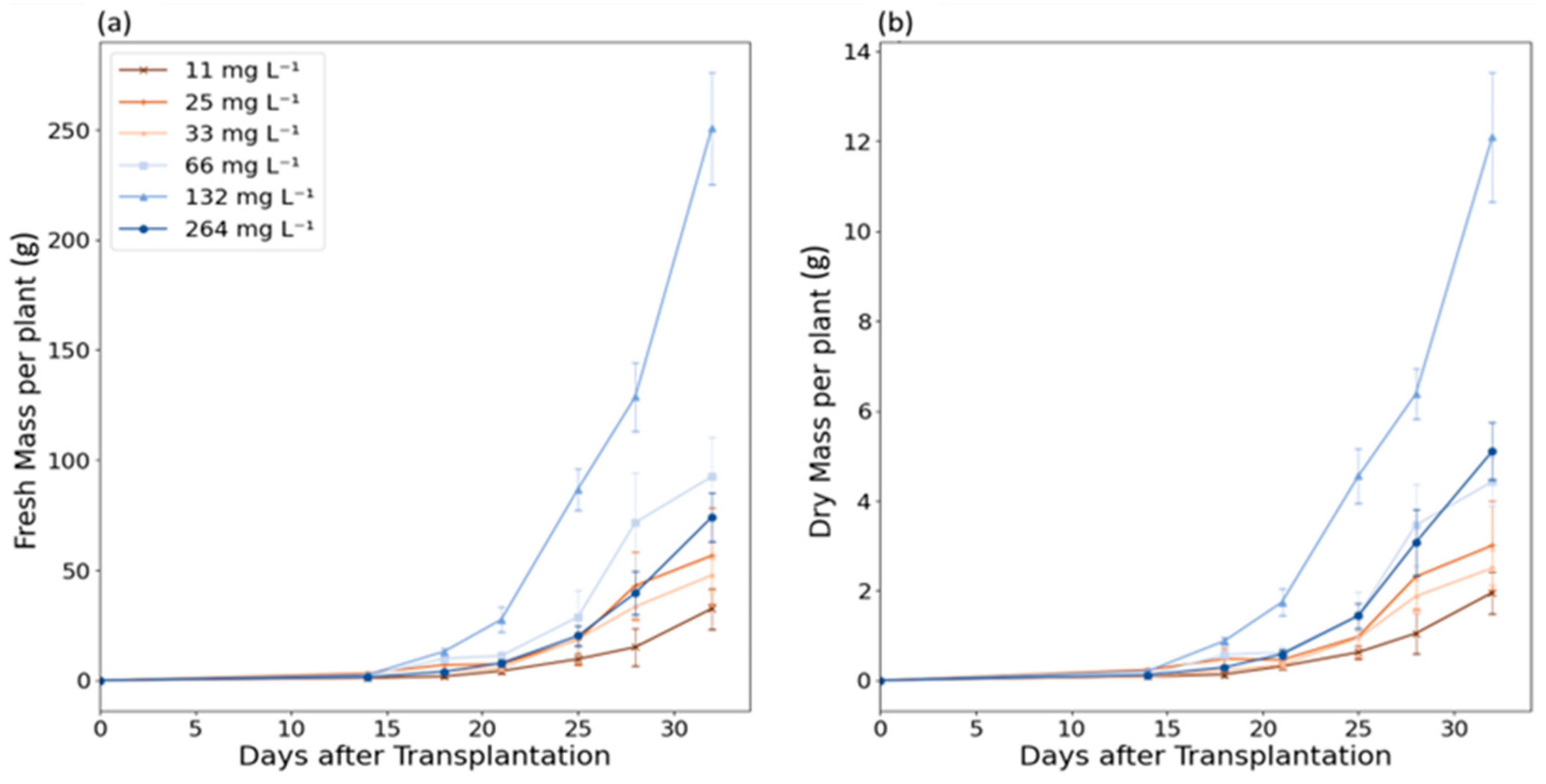
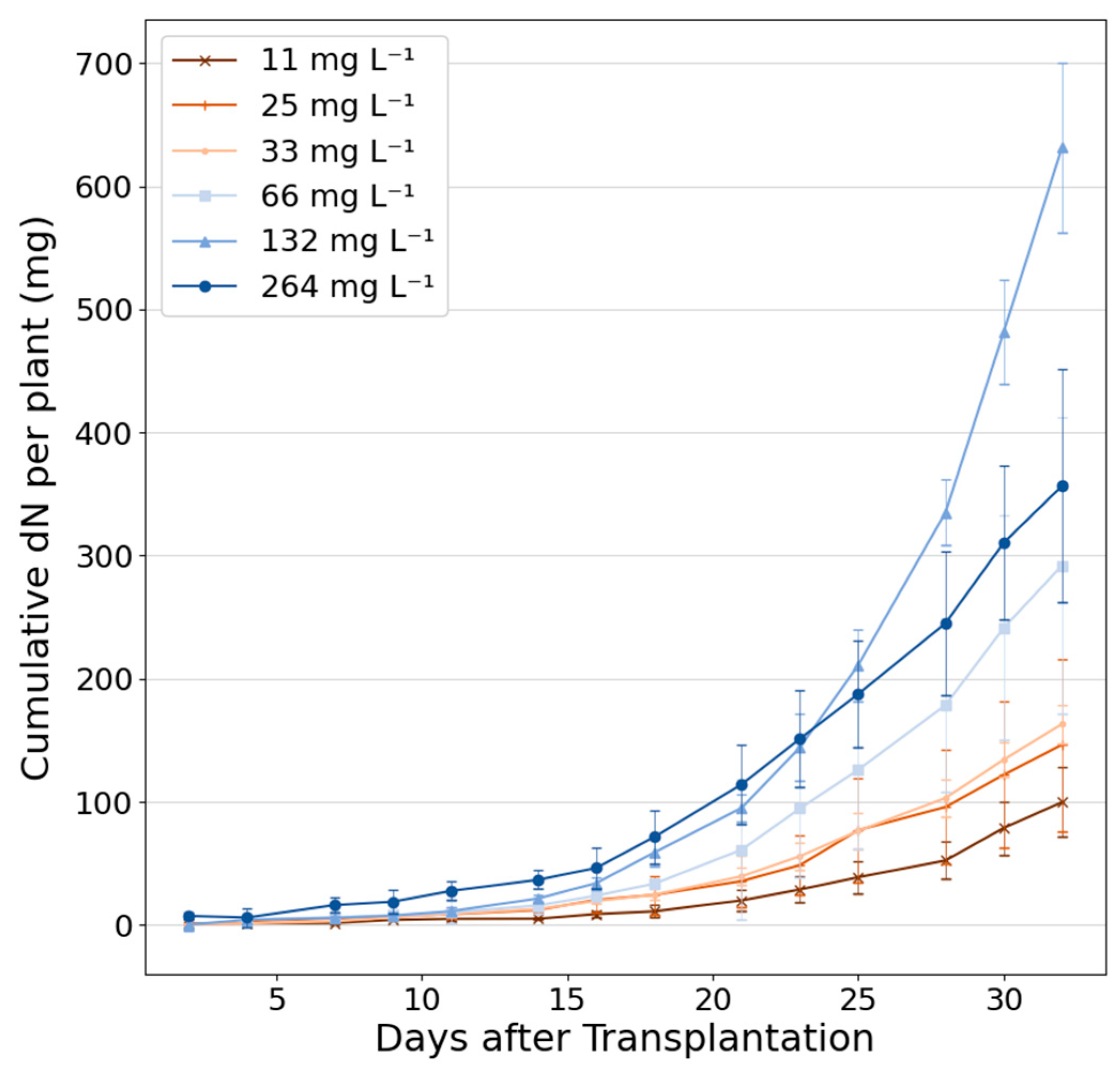
3.1. Biomass Growth and Nitrogen Depletion

Table 3. Fresh mass (top), dry mass (bottom), and dry mass %.

DAT	11 mg L−1	25 mg L−1	33 mg L−1	66 mg L−1	132 mg L−1	264 mg L−1
14	0.96 ± 0.33	3.20 ± 0.46	1.13 ± 0.16	2.00 ± 0.51	2.61 ± 0.48	1.53 ± 0.33
	0.08 ± 0.03 (8.3%)	0.24 ± 0.03 (7.5%)	0.09 ± 0.01 (8.0%)	0.13 ± 0.02 (6.5%)	0.21 ± 0.04 (8.0%)	0.12 ± 0.02 (7.8%)
18	1.85 ± 0.77	7.04 ± 3.80	4.13 ± 0.67	9.94 ± 1.56	13.07 ± 1.24	4.00 ± 0.73
	0.14 ± 0.06 (7.6%)	0.48 ± 0.22 (6.8%)	0.23 ± 0.03 (5.6%)	0.57 ± 0.07 (5.7%)	0.88 ± 0.09 (6.7%)	0.29 ± 0.05 (7.3%)
21	4.29 ± 1.05	7.37 ± 2.32	5.61 ± 1.28	11.20 ± 1.81	27.63 ± 5.67	7.84 ± 1.70
	0.31 ± 0.07 (7.2%)	0.46 ± 0.11 (6.2%)	0.35 ± 0.08 (6.2%)	0.62 ± 0.14 (5.5%)	1.74 ± 0.30 (6.3%)	0.58 ± 0.11 (7.4%)
25	9.68 ± 2.39	18.46 ± 11.40	18.79 ± 3.18	28.74 ± 12.30	86.81 ± 9.44	20.23 ± 4.68
	0.63 ± 0.14 (6.5%)	0.98 ± 0.47 (5.3%)	0.94 ± 0.16 (5.0%)	1.45 ± 0.51 (5.0%)	4.55 ± 0.61 (5.2%)	1.44 ± 0.28 (7.1%)
28	15.1 ± 8.48	43.07 ± 15.09	33.51 ± 6.40	71.63 ± 22.52	128.71 ± 15.45	39.64 ± 9.82
	1.05 ± 0.45 (7.0%)	2.31 ± 0.73 (5.4%)	1.87 ± 0.36 (5.6%)	3.46 ± 0.92 (4.8%)	6.38 ± 0.56 (5.0%)	3.07 ± 0.73 (7.7%)
32	32.57 ± 9.22	56.62 ± 21.95	47.73 ± 7.35	92.53 ± 17.97	250.73 ± 25.41	74.11 ± 10.90
	1.96 ± 0.47 (6.0%)	3.00 ± 0.99 (5.3%)	2.50 ± 0.39 (5.2%)	4.42 ± 0.54 (4.8%)	12.10 ± 1.44 (4.8%)	5.10 ± 0.64 (6.9%)

Sample sizes for each cell vary, ranging from n = 3 to n = 40, with an average of n = 13.

illustrates the biomass growth profiles and 95% confidence intervals for each harvest. These measurements confirm that inorganic nitrogen concentrations of the baseline MSS yielded the greatest fresh (250.73 ± 25.41 g) and dry mass (12.10 ± 1.44 g) on 32 DAT. While lesser concentrations produced lower fresh and dry mass, these trends are not entirely consistent, with the 25 mg L⁻¹ treatment on average outperforming the 33 mg L⁻¹ treatment, albeit within the margin of error. This may be explained by limited samples and hydroponic systems when conducting the 25 mg L⁻¹ treatment, combined with biological and environmental differences.

While both fresh and dry mass increased throughout the growth cycle of each treatment, these returns began to diminish after 28 DAT for most under-fertilized treatments (Figure 2). This minor change suggests that under-fertilized plants may be entering the mature growth phase. Regardless, amongst nutrient-rich treatments, researchers noticed that lettuce was still growing strongly upon final harvest on 32 DAT. This suggests extending the growth period in future testing.

As nutrient concentrations increased, fresh and dry biomass increased consistently up to the 132 mg L⁻¹ (baseline MSS) treatment. However, the 264 mg L⁻¹ treatment demonstrated a decrease in fresh and dry mass from the 132 mg L⁻¹ treatment. This decrease, as well as an increase in dry mass % between the two treatments, indicates these tissue samples held less water, producing smaller and more nutrient-dense lettuce shoots. However, the mechanism responsible for this change in composition requires further study. Overall, the results of the 264 mg L⁻¹ treatment support the MSS baseline nitrogen concentration, and support that increased fertilizer concentrations do not necessarily yield higher productivity, especially when exceeding a crop’s nutrient requirements.

Similar to biomass growth, nitrogen depletion per plant (Figure 3) also increased with respect to crop age and total nitrogen concentration up to the 132 mg L⁻¹ treatment. Interestingly, unlike other treatments, the 264 mg L⁻¹ showed significant nitrogen depletion beginning on 7 DAT. However, the absence of corresponding plant tissue growth during this period indicates a nitrogen loss disparity. This may be explained by increased root or microbial growth in a high-nutrient environment. While roots were unmeasurable in the current system, researchers observed biofilms growing inside the darkened tubing as well as photosynthetic biofilms growing on all wet internal surfaces throughout the study, especially during nutrient-rich treatments. Another potential factor could be the denitrification of N₂ or N₂O gas [73,74]. While this may be less likely to occur in an aerobic environment, it is of significant interest to many environmental engineers and more research is needed. However, these measurements were beyond the scope and toolset of this study.

Most of the direct measurements of this study focus on biomass quantity and not quality. However, nutrient-limited crops not only have the potential to be smaller but also exhibit signs of malnutrition, such as yellow leaves, brown spots, flimsy texture, and bitter taste, which may make them unpalatable [67,75]. Figure 4 provides visual examples of model lettuce from four of these treatments.

Cataloging visual differences was not a primary objective in this study. Regardless, throughout experimentation, researchers noted plant characteristics from all $\ge$66 mg L⁻¹ treatments appeared healthy throughout growth, exhibiting less noticeable malnourishment (e.g., yellow leaves, spotting) than that observed in the $\le$33 mg L⁻¹ treatments. These observations support previously mentioned findings in established literature.

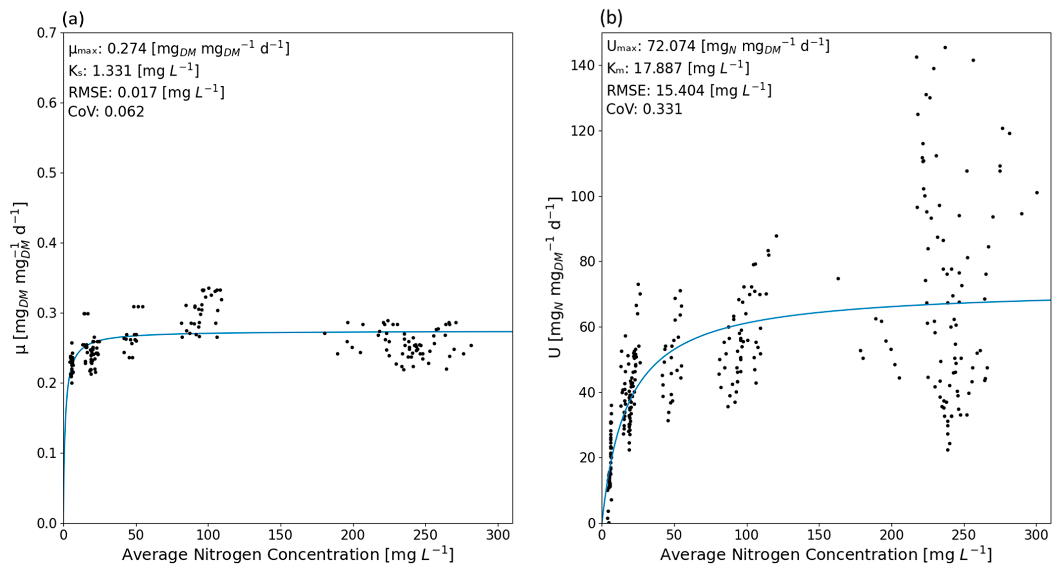
3.2. Monod and Michaelis–Menten Modeling

Figure 5a,b illustrate Monod and Michaelis–Menten curves, respectively. Coefficient of Variance (CoV) values were also determined to evaluate predictive performance and were achieved by dividing the standard deviation of the model prediction by the mean of the dependent variable.

The Monod curve identified a maximum specific growth rate of 0.274 $\mathrm{m}{\mathrm{g}}_{\mathrm{D}\mathrm{M}} {\mathrm{mg}}_{\mathrm{D}\mathrm{M}}^{-1} {\mathrm{d}}^{-1}$ and $K_s$ = 1.331 mg L⁻¹. The peak in growth rate at the 132 mg L⁻¹ treatment supports the MSS baseline as the optimal nitrogen substrate concentration. Furthermore, the slight decrease in growth rate at elevated concentrations may be attributed to inhibitory effects via Haldane kinetics.

The low $K_s$ value indicates an exceptionally low nitrogen concentration at 1.331 mg L⁻¹ is required to produce half of the maximum growth rate. Of course, farmers are not necessarily interested in growing produce at half-speed. Still, this is a promising indicator that low-nutrient sources, such as reclaimed wastewater at 40–60 mg L⁻¹ nitrogen, may approximate a maximum growth rate of around ~0.27 $\mathrm{m}{\mathrm{g}}_{\mathrm{D}\mathrm{M}} {\mathrm{mg}}_{\mathrm{D}\mathrm{M}}^{-1} {\mathrm{d}}^{-1}$, fulfilling quantitative biomass demands of agriculture.

As a hypothetical example, a similar hydroponic environment may be chosen to provide a constant 60 $\mathrm{m}{\mathrm{g}}_{\mathrm{N}} {\mathrm{L}}^{-1}$ to their Bibb lettuce. This concentration represents the upper range of the expected nitrogen concentrations in wastewater and 45% of the optimal MSS baseline nitrogen concentration. By plugging ${\mu }_{\mathit{max}}, K_s,$ and $\left[N\right]$ into Equation (2), we can estimate µ as 0.268 $\mathrm{m}{\mathrm{g}}_{\mathrm{D}\mathrm{M}} \mathrm{m}{\mathrm{g}}_{\mathrm{D}\mathrm{M}}^{-1} {\mathrm{d}}^{-1}$. By entering this along with $D{M}_0, t_0, \mathrm{a}\mathrm{n}\mathrm{d} t_h$ into Equation (5), we can estimate plant dry mass on a given day. In the example of $t_h=32$ DAT, the resulting Bibb lettuce can be expected to approximate 11.68 ${\mathrm{g}}_{\mathrm{D}\mathrm{M}}$. If we compare this result to the 66 mg L⁻¹ treatment in Table 3 and the corresponding images in Figure 4, we can see that this estimate far exceeds that treatment’s measured $4.42\pm 0.54 {\mathrm{g}}_{\mathrm{DM}}$, yet closely approximates the MSS baseline 132 mg L⁻¹ treatment of $12.10\pm 1.44{ \mathrm{g}}_{\mathrm{DM}}$ and corresponding fresh mass of 250.73 ± 25.41 g (approximately 8.8 oz). While these are the best-fit parameters based on available data, including all treatments and time points, they can be a poor predictor for lower nitrogen substrate concentrations. This represents one of the greatest shortcomings of this model and highlights the potential need for additional data points and an improved model for predicting total biomass.

This shortcoming with low nutrient treatments can be attributed to the low $K_s$ which is visually discerned by a relatively flat curve. To increase confidence in this parameter, researchers may first wish to conduct additional experiments with ultra-low concentrations. However, these low concentrations pose a challenge for practical experimentation, as producing a nutrient solution that is significantly deficient in dissolved inorganic nitrogen often sacrifices either other vital nutrients or pH.

Meanwhile, the Michaelis-Menten model identifies a maximum specific uptake rate of 72.074 $\mathrm{m}{\mathrm{g}}_{\mathrm{N}} \mathrm{m}{\mathrm{g}}_{\mathrm{D}\mathrm{M}}^{-1} {\mathrm{d}}^{-1}$ and $K_m$ = 17.887 mg L⁻¹. This fails to demonstrate similar substrate affinity $K_s$ and Michaelis $K_m$ constants (e.g., $K_s$ ≠ $K_m$), which may be explained by a shift in the production of non-nitrogenous tissues during low concentrations. Such an occurrence would result in still-elevated total biomass growth when nitrogen uptake is low, potentially suggesting a measurable qualitative difference in tissue dependent on substrate concentration. And while biomass production quantity may be a primary goal of farmers when profits are driven by weight, it is crucial to maintain product quality, as sickly or bitter lettuce is unappealing to consumers. This will be further explored in shoot-specific cell yield $Y_{shoot}$.

It is important to note that the Michaelis-Menten model depends upon accurate estimation of biomass in the system, and alternative methods to estimate biomass, whether destructive or non-destructive, will significantly affect the estimated value of the maximum uptake rate.

Additionally, it should be acknowledged that the original baseline recipe from the literature composed 5% of total nitrogen as ammonium, with the rest as nitrate, during synthesis. The 66 mg L⁻¹ recipe reduced this to 1.8%, and the remaining low-nitrogen recipes to zero ammonium. Meanwhile, the 264 mg L⁻¹ treatment composed of a large 27.5% ammonium, which may be a contributing factor to the observed decreased growth. However, this treatment’s inclusion or exclusion from the modeling software had little impact on the value of kinetic parameters that best fit the remaining data.

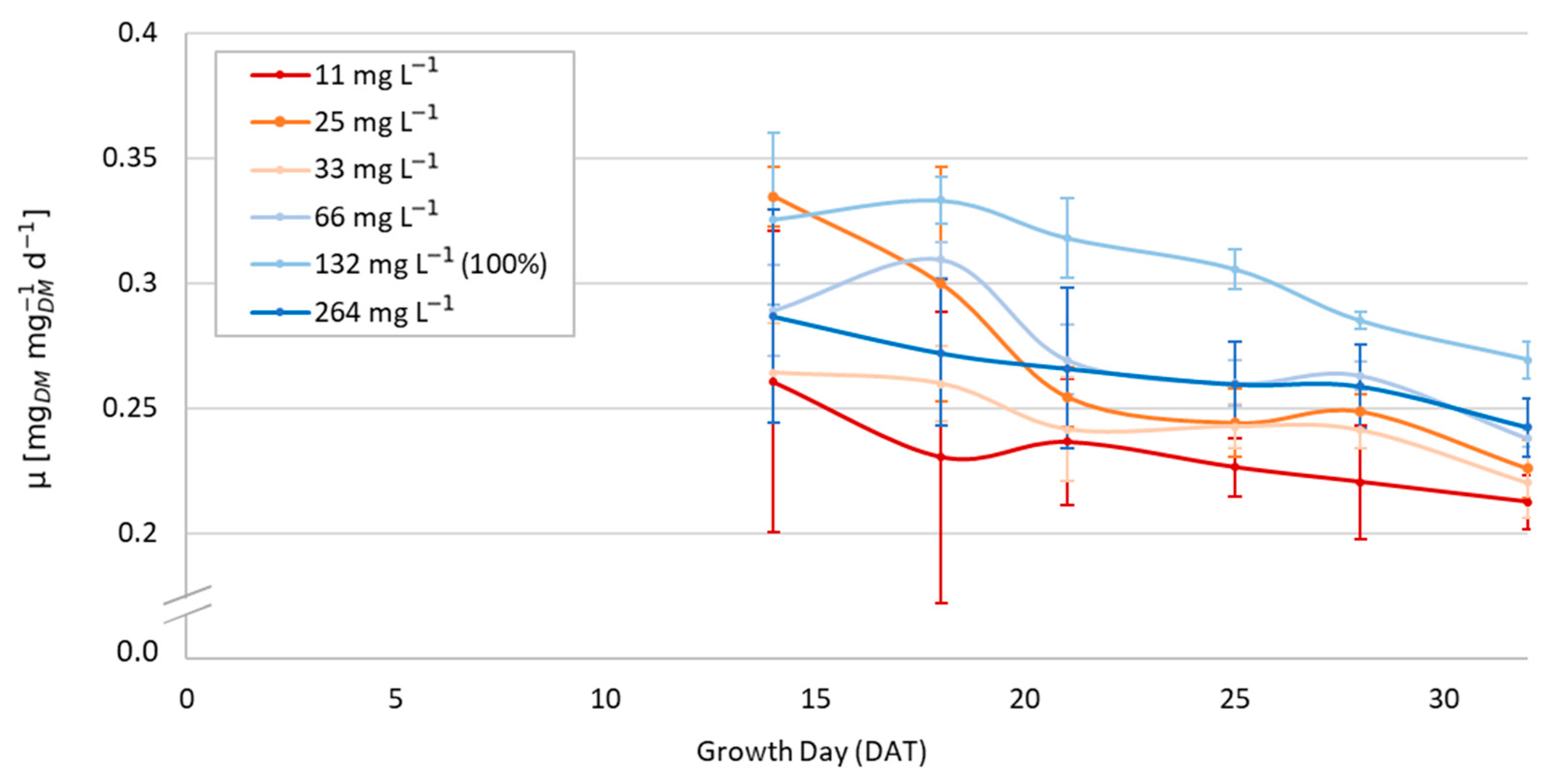
3.3. Dynamic Growth Rates

As previously mentioned, specific growth rates were observed to be temporally variable, decreasing during each treatment as the plants matured (Figure 6).

This may indicate that a specific growth rate may be best represented as a function rather than a constant. While similar behavior may be present within microbial systems on an individual level, such observations would likely be hidden by rapid reproduction and multiple concurrent generations, resulting in a lifetime average specific growth rate across the population.

How could this potentially affect our previous hydroponic example at 60 mg L⁻¹? It would be conceivable that an initial (young plant) specific growth rate that is exceptionally high may accurately reflect in a Monod curve with a much higher ${\mu }_{max}$ that decreases as the plant matures. If this was attempted to be translated into a temporally independent Monod curve, as performed here, we would expect the appearance of an exceptionally low $K_s$ that would overestimate the growth of low-nutrient treatments and either match or underestimate the growth of treatments receiving optimal nutrient concentrations. This supports the need for future investigation into a dynamic Monod model, which is temporally dependent on the plant’s lifecycle.

To support such a model, future hydroponic research should include measurement of young plants (e.g., <14 DAT) to allow researchers to more strongly identify specific growth rates across the entire Bibb lettuce lifecycle. The additional data from the first half of the plant lifecycle can increase confidence in the nature of this relationship and create a dynamic Monod model, thereby improving biomass estimations across concentration and plant age as well as nutrient uptake. The observed deviations in the 25 mg L⁻¹ and 66 mg L⁻¹ treatments can be attributed to the same low sample quantity explanation as discussed regarding dry mass measurements in Table 3.

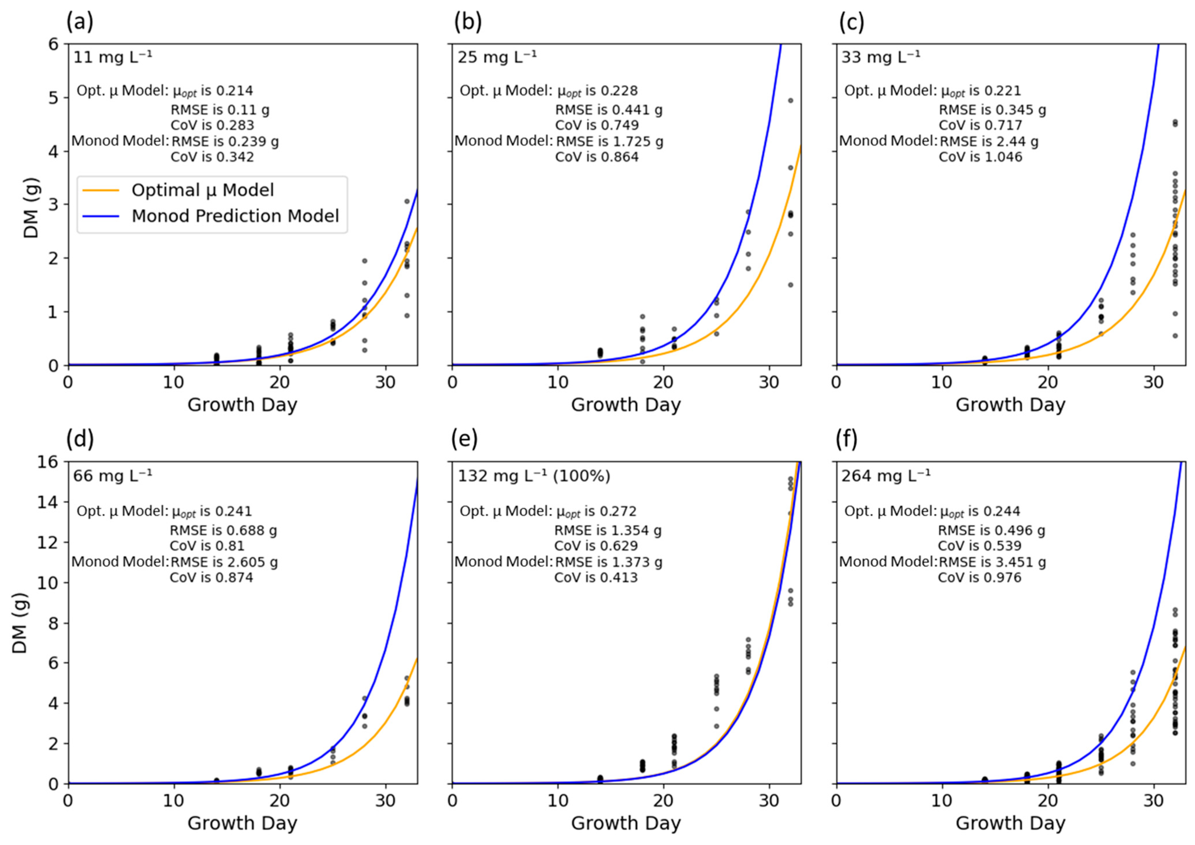
3.4. Visualizing Growth Models

Figure 7 compares the predictive capability of the Monod model against the Optimal µ model and dry mass measurements.

A comparison of the two biomass models reveals that the Optimal µ model offers improved predictive capability, with lower RMSE values across all treatments. However, this is expected as each Optimal µ model functions independently to best fit the dry mass data within each treatment. Meanwhile, the Monod model ties all treatments together via a single set of parameters.

This Monod model significantly overestimates the 25, 33, and 66 mg L⁻¹ treatments. Meanwhile, the overestimation in the 264 mg L⁻¹ treatment may be attributed to inhibition via Haldane kinetics. However, this inhibition is outside the scope of this study, and researchers would recommend at least one additional over-fertilized treatment to quantify this parameter.

Similar to overestimating biomass in under-fertilized treatments, this Monod model also underestimates biomass in early life but improves or overestimates biomass after 25 DAT. This temporal shift from underestimation to overestimation further supports that a dynamic µ that begins high and decreases over a plant’s lifecycle may be required for accurate biomass prediction of lettuce.

3.5. Shoot-Specific Cell Yield

Cell yield can be an important ratio for hydroponic operations, as tracking biomass growth per nutrient uptake is a primary step in calculating revenue per cost for a given crop. This ratio can be utilized to determine optimal nutrient concentrations or harvest times. The shoot-specific cell yield $Y_{shoot}$ utilized nitrogenous shoot tissue as a proxy for nitrogen uptake due to the nitrogen loss disparity, as indicated previously, and results are shown in Figure 8.

When observing Figure 8a for optimal harvest times, each treatment shows a general decrease in shoot-specific cell yield between days 14 and 25, followed by a slight increase until the final harvests on day 32. This elevated cell yield was most significant with low nitrogen treatments (with average nitrogen $\le$26.2 mg L⁻¹). Meanwhile, high nitrogen treatments (with average nitrogen $\ge$41.7 mg L⁻¹) experienced a relatively constant yield of $17.77\pm 0.26 {\mathrm{g}}_{\mathrm{DM}} {\mathrm{g}}_{\mathrm{N}}^{-1}$ with increased variation above 150 mg L⁻¹. This distinction between high and low nitrogen treatments is easily visualized in Figure 8b. Furthermore, because $Y_{shoot}$ directly measures nitrogenous biomass, the elevated values seen in low nitrogen conditions indicate that lettuce composition is affected by nitrogen substrate concentration and demonstrate the threshold at which the negative effects of insufficient nutrients surpass producing smaller crop biomass (quantity) and begin impacting lettuce composition (quality). These measurements correspond with visual observations of nitrogen deficiency seen in the photographs in Figure 4.

The increased yield at nitrogen-deficient concentrations may first appear counterintuitive. This observation can be explained by plants’ inability to produce nitrogenous tissues while maintaining the relative production of non-nitrogenous tissues when nitrogen substrate is scarce. Unless limiting nutrients inhibit all biomass production, researchers should expect cell yield to increase during nutrient deprivation.

Following our prior example of the hydroponic farm operating at 60 $\mathrm{m}{\mathrm{g}}_{\mathrm{N}} {\mathrm{L}}^{-1}$, we would expect the Bibb lettuce to have a $Y_{shoot}$ of approximately 18 ${\mathrm{g}}_{\mathrm{DM}} {\mathrm{g}}_{\mathrm{N}}^{-1}$, bearing similarity to nutrient-rich treatments. And while the model appears to overestimate dry mass quantity, the estimated shoot-specific cell yield is supported by the images in Figure 4, which produced smaller lettuce but showed no additional signs of nitrogen deficiency.

While prior studies have established optimal nitrogen for total lettuce biomass growth and general plant nutrition as 130–220 mg L⁻¹ [59,76,77,78,79,80], the results presented here identify and quantify the minimum threshold to produce compositionally healthy Bibb lettuce as between 26.2 and 41.7 mg L⁻¹. Assuming other growth conditions are satisfied, lettuce grown above this minimum threshold but below 130–150 mg L⁻¹ may be expected to be compositionally healthy, albeit with smaller total biomass. Furthermore, this potential minimum threshold approximates the lower bound of the previously discussed wastewater nitrogen content of 40–60 mg L⁻¹. While the difference between the minimum threshold and this expected wastewater nitrogen leaves little room for safety factors when designing wastewater recovery systems (e.g., due to dilution processes or below-average nitrogen influent), it nonetheless supports the potential use of reclaimed wastewater as a source of nitrogen for hydroponic agriculture. However, to maintain maximized biomass growth, wastewater may require either supplemental nutrients or supplemental processes to concentrate existing nutrients to optimal levels.

3.6. Final Considerations

As noted by Wheeler et al., the parameters derived from this study are relevant for this specific environment as they are dependent on environmental control inputs and growth conditions [46]. One significant factor of these growth conditions is the influence of vertical farming, which may pressure plants to allocate additional energy and nutrients for structural support to oppose perpendicular gravitational forces. Therefore, further experiments will be required both to evaluate root biomass growth and to translate these parameter values to alternative growth environments such as deep-water culture.

Additionally, the evaluation of other nutrients and higher-order molecular constituents, the inclusion of root measurements, <14 DAT and >32 DAT harvests, and low nitrogen concentrations would significantly improve model value, potentially helping to identify the nitrogen loss disparity between nutrient solution samples and tissue harvests. And while it currently stands as speculation, it is possible a dynamic $\mu$ may be applicable for biomass prediction at an individual level for other organisms, including within microbial populations. However, eliminating the reproduction and synchronizing the lifecycles of microbes may pose a significant challenge and offer little practical benefit for populations that generally exist in such massive and diverse numbers.

The greatest physical challenge in hydroponic kinetics involves the complex task of maintaining constant nutrient concentrations in hydroponic systems, which are depleted quickly in low-nitrogen treatments. Such depletion may invoke plant response in nutrient uptake once additional nutrients are provided, potentially explaining the high uptake values in the 11 mg L⁻¹ treatment. These shortcomings in experimental design may be mitigated with shorter intervals between water changes at the expense of significantly higher costs and increased labor. Further treatments supplying approximately 1–2 mg L⁻¹ nitrogen would also better confirm $K_s$ and $K_m$ values in the same range. While this could be accomplished utilizing a continuous flow reactor or peristaltic dosing pumps, our researchers recommend increasing the system volume per plant.

Lastly, it’s important to acknowledge the complexity of wastewater, modeling, and its use in agriculture. Such substrates comprise more than just a series of inorganic nutrients/elements. Factors for additional consideration include growth inhibitors, electrical conductivity, heavy metals, surfactants, antibiotics and contaminants of emerging concern, dissolved oxygen, chemical oxygen demand, carbon content, swings in pH and salinity, competition from heterotrophs, and pathogen transport and influence. Further research can begin to combine the factors and document their interactions.

4. Conclusions

This study demonstrates that mechanistic models built on a priori knowledge of first principles can be functionally applied to hydroponically grown Bibb lettuce. However, it reveals the need for future models to incorporate dynamic, rather than constant, specific biomass growth and nutrient uptake rates to make accurate predictions at all life stages. Furthermore, linking Michaelis-Menten uptake kinetics to Monod growth kinetics establishes a foundational set of procedures, analytical methods, and model parameters for future hydroponic and waste-to-food agronomic research. Finally, in the weighing of quantity vs. quality, these results support that the nitrogen content of reclaimed wastewater may be expected to produce smaller but nutritionally healthy lettuce in similar vertical hydroponic environments.

References

1. Halal, W.E.; Davies, O. State of the future, 19.0. World Futures Rev. 2018, 10, 95–98. [Google Scholar] [CrossRef]
2. National Academies of Sciences, Engineering, and Medicine. Environmental Engineering for the 21st Century: Addressing Grand Challenges; National Academies Press: Washington, DC, USA, 2019; ISBN 978-0-309-47652-2. [Google Scholar]
3. NAE Grand Challenges for Engineering: 14 Grand Challenges for Engineering in the 21st Century; National Academy of Engineering: Washington, DC, USA, 2006.
4. Enriquez, J.P. Food self-sufficiency: Opportunities and challenges for the current food system. Biomed. J. Sci. Tech. Res. 2020, 31, 23984–23989. [Google Scholar] [CrossRef]
5. Kaviti, G.; Asadu, C.; Wiseman, P. Russian war worsens fertilizer crunch, risking food supplies. Associated Press News, 12 April 2022. [Google Scholar]
6. Zhang, W.; Ma, W.; Ji, Y.; Fan, M.; Oenema, O.; Zhang, F. Efficiency, economics, and environmental implications of phosphorus resource use and the fertilizer industry in china. Nutr. Cycl. Agroecosyst. 2008, 80, 131–144. [Google Scholar] [CrossRef]
7. Steen, I.; Agro, K. Phosphorus availability in the 21st century—Management of a non-renewable resource. Phosphorus Potassium 1998, 217, 25–31. [Google Scholar]
8. Hosseinian, A.; Pettersson, A.; Ylä-Mella, J.; Pongrácz, E. Phosphorus recovery methods from secondary resources, assessment of overall benefits and barriers with focus on the nordic countries. J. Mater. Cycles Waste Manag. 2023, 25, 3104–3116. [Google Scholar] [CrossRef]
9. Snyder, C.S.; Bruulsema, T.W.; Jensen, T.L.; Fixen, P.E. Review of greenhouse gas emissions from crop production systems and fertilizer management effects. Agric. Ecosyst. Environ. 2009, 133, 247–266. [Google Scholar] [CrossRef]
10. Madigan, M.T.; Martinko, J.M.; Bender, K.S.; Buckley, D.H.; Stahl, D.A. Brock Biology of Micro-Organisms, 14th ed.; Pearson: London, UK, 1992; ISBN 9780321897398. [Google Scholar]
11. Gellings, C.W.; Parmenter, K.E. Energy efficiency in fertilizer production and use. In Efficient Use and Conservation of Energy: Encyclopedia of Life Support Systems; EOLSS Publishers: Oxford, UK, 2004. [Google Scholar]
12. Kool, A.; Marinussen, M.; Blonk, H. LCI Data for the Calculation Tool Feedprint for Greenhouse Gas Emissions of Feed Production and Utilization: GHG Emissions of N, P and K Fertilizer Production; Blonk Consultants: Gouda, The Netherlands, 2012. [Google Scholar]
13. FAO. “Energy-Smart” Food for People and Planet; FAO: Rome, Italy, 2011. [Google Scholar]
14. Brown, B.D.; Engel, R.; Management, N.; Olson-Rutz, K.; Associate, R. Management to Minimize Nitrogen Fertilizer Volatilization; Montana State University: Bozeman, MT, USA, 2020. [Google Scholar]
15. Dawson, C.J.; Hilton, J. Fertiliser availability in a resource-limited world: Production and recycling of nitrogen and phosphorus. Food Policy 2011, 36, S14–S22. [Google Scholar] [CrossRef]
16. Takaya, N.; Catalan-Sakairi, M.A.B.; Sakaguchi, Y.; Kato, I.; Zhou, Z.; Shoun, H. Aerobic denitrifying bacteria that produce low levels of nitrous oxide. Appl. Environ. Microbiol. 2003, 69, 3152–3157. [Google Scholar] [CrossRef] [PubMed]
17. Soussana, J.F.; Allard, V.; Pilegaard, K.; Ambus, P.; Amman, C.; Campbell, C.; Ceschia, E.; Clifton-Brown, J.; Czobel, S.; Domingues, R.; et al. Full accounting of the greenhouse gas (CO2, N2O, CH4) budget of nine european grassland sites. Agric. Ecosyst. Environ. 2007, 121, 121–134. [Google Scholar] [CrossRef]
18. Kaye, J.P.; Groffman, P.M.; Grimm, N.B.; Baker, L.A.; Pouyat, R.V. A distinct urban biogeochemistry? Trends Ecol. Evol. 2006, 21, 192–199. [Google Scholar] [CrossRef]
19. Krauter, C.T.; Potter, C.; Klooster, S. Ammonia Emission Related to Nitrogen Fertilizer Application Practices. In Proceedings of the California Department of Food and Agriculture Fertilizer Education Program Conference, Tulare, CA, USA, 2001. [Google Scholar]
20. Lammel, G.; Graßl, H. Greenhouse effect of NOX. Environ. Sci. Pollut. Res. 1995, 2, 40–45. [Google Scholar] [CrossRef] [PubMed]
21. Müller, R. The impact of the rise in atmospheric nitrous oxide on stratospheric ozone. Ambio 2021, 50, 35–39. [Google Scholar] [CrossRef]
22. Shine, K.P. Radiative forcing of climate change. Space Sci. Rev. 2000, 94, 363–373. [Google Scholar] [CrossRef]
23. Tian, H.; Xu, R.; Canadell, J.G.; Thompson, R.L.; Winiwarter, W.; Suntharalingam, P.; Davidson, E.A.; Ciais, P.; Jackson, R.B.; Janssens-Maenhout, G.; et al. A comprehensive quantification of global nitrous oxide sources and sinks. Nature 2020, 586, 248–256. [Google Scholar] [CrossRef] [PubMed]
24. Berg, M.; Koskella, B. Nutrient- and dose-dependent microbiome-mediated protection against a plant pathogen. Curr. Biol. 2018, 28, 2487–2492.e3. [Google Scholar] [CrossRef] [PubMed]
25. Richardson, D.; Felgate, H.; Watmough, N.; Thomson, A.; Baggs, E. Mitigating release of the potent greenhouse gas N2O from the nitrogen cycle—Could enzymic regulation hold the key? Trends Biotechnol. 2009, 27, 388–397. [Google Scholar] [CrossRef] [PubMed]
26. Rufí-Salís, M.; Petit-Boix, A.; Villalba, G.; Sanjuan-Delmás, D.; Parada, F.; Ercilla-Montserrat, M.; Arcas-Pilz, V.; Muñoz-Liesa, J.; Rieradevall, J.; Gabarrell, X. Recirculating water and nutrients in urban agriculture: An opportunity towards environmental sustainability and water use efficiency? J. Clean. Prod. 2020, 261, 121213. [Google Scholar] [CrossRef]
27. Li, W.; Yu, H.; Rittmann, B.E. Reuse water pollutants. Nature 2015, 528, 29–31. [Google Scholar] [CrossRef]
28. Chojnacka, K.; Witek-Krowiak, A.; Moustakas, K.; Skrzypczak, D.; Mikula, K.; Loizidou, M. A transition from conventional irrigation to fertigation with reclaimed wastewater: Prospects and challenges. Renew. Sustain. Energy Rev. 2020, 130, 109959. [Google Scholar] [CrossRef]
29. Muhaidat, R.; Al-Qudah, K.; Al-Taani, A.A.; AlJammal, S. Assessment of nitrate and nitrite levels in treated wastewater, soil, and vegetable crops at the upper reach of Zarqa river in Jordan. Environ. Monit. Assess. 2019, 191, 153. [Google Scholar] [CrossRef]
30. McClintock, S.A.; Sherrard, J.H.; Novak, J.T.; Randall, C.W. Nitrate versus oxygen respiration in the activated sludge process. J. Water Pollut. Control Fed. 1988, 60, 342–350. [Google Scholar]
31. Tomei, M.C.; Carozza, N.A.; Mosca Angelucci, D. Post-aerobic digestion of waste sludge: Performance analysis and modelling of nitrogen fate under alternating aeration. Int. J. Environ. Sci. Technol. 2016, 13, 21–30. [Google Scholar] [CrossRef]
32. Lee, E.; Rout, P.R.; Bae, J. The applicability of anaerobically treated domestic wastewater as a nutrient medium in hydroponic lettuce cultivation: Nitrogen toxicity and health risk assessment. Sci. Total Environ. 2021, 780, 146482. [Google Scholar] [CrossRef]
33. Lei, M.; Zhang, L.; Lei, J.; Zong, L.; Li, J.; Wu, Z.; Wang, Z. Overview of emerging contaminants and associated human health effects. Biomed. Res. Int. 2015, 2015, 404796. [Google Scholar] [CrossRef] [PubMed]
34. Kelemen, D.I. Uptake of Common Pharmaceutical Compounds in Hydroponically Grown Lactuca sativa. Master’s Thesis, University of Connecticut, Storrs, CT, USA, 2018. [Google Scholar]
35. Altieri, M.A.; Nicholls, C.I. Sustainable Agriculture Reviews; Springer: Berlin/Heidelberg, Germany, 2012; Volume 11, ISBN 978-94-007-5448-5. [Google Scholar]
36. Hoque, M.M.; Ajwa, H.A.; Smith, R. Nitrite and ammonium toxicity on lettuce grown under hydroponics. Commun. Soil. Sci. Plant Anal. 2007, 39, 207–216. [Google Scholar] [CrossRef]
37. Savvas, D.; Passam, H.C.; Olympios, C.; Nasi, E.; Moustaka, E.; Mantzos, N.; Barouchas, P. Effects of ammonium nitrogen on lettuce grown on pumice in a closed hydroponic system. HortScience 2006, 41, 1667–1673. [Google Scholar] [CrossRef]
38. McCall, D.; Willumsen, J. Effects of nitrate, ammonium and chloride application on the yield and nitrate content of soil-grown lettuce. J. Hortic. Sci. Biotechnol. 1998, 73, 698–703. [Google Scholar] [CrossRef]
39. Wang, B.; Shen, Q. Effects of ammonium on the root architecture and nitrate uptake kinetics of two typical lettuce genotypes grown in hydroponic systems. J. Plant Nutr. 2012, 35, 1497–1508. [Google Scholar] [CrossRef]
40. Zhang, K.; Burns, I.G.; Turner, M.K. Derivation of a dynamic model of the kinetics of nitrogen uptake throughout the growth of lettuce: Calibration and validation. J. Plant Nutr. 2008, 31, 1440–1460. [Google Scholar] [CrossRef]
41. Schröder, J.J.; Smit, A.L.; Cordell, D.; Rosemarin, A. Improved phosphorus use efficiency in agriculture: A key requirement for its sustainable use. Chemosphere 2011, 84, 822–831. [Google Scholar] [CrossRef]
42. Yu, H.Y.; Li, T.X.; Zhang, X.Z. Nutrient budget and soil nutrient status in greenhouse system. Agric. Sci. China 2010, 9, 871–879. [Google Scholar] [CrossRef]
43. Epstein, E.; Hagen, C.E. A kinetic study of the absorption of alkali cations by barley roots. Plant Physiol. 1951, 27, 457–474. [Google Scholar] [CrossRef] [PubMed]
44. Griffiths, M.; York, L.M. Targeting root ion uptake kinetics to increase plant productivity and nutrient use efficiency. Plant Physiol. 2020, 182, 1854–1868. [Google Scholar] [CrossRef] [PubMed]
45. Barber, S.A.S. Soil Nutrient Bioavailability: A Mechanistic Approach, 1st ed.; John Wiley & Sons, Inc.: New York, NY, USA, 1984. [Google Scholar]
46. Wheeler, E.F.; Albright, L.D.; Spanswick, R.M.; Walker, L.P.; Langhans, R.W. Nitrate uptake kinetics in lettuce as influenced by light and nitrate nutrition. Trans. ASAE 1998, 41, 859–867. [Google Scholar] [CrossRef]
47. Monod, J. The growth of bacterial cultures. Annu. Rev. Microbiol. 1949, 3, 371–394. [Google Scholar] [CrossRef]
48. Strigul, N.; Dette, H.; Melas, V.B. A practical guide for optimal designs of experiments in the Monod model. Environ. Model. Softw. 2009, 24, 1019–1026. [Google Scholar] [CrossRef]
49. Grosfils, A.; Vande Wouwer, A.; Bogaerts, P. On a general model structure for macroscopic biological reaction rates. J. Biotechnol. 2007, 130, 253–264. [Google Scholar] [CrossRef] [PubMed]
50. Seginer, I.; Buwalda, F.; van Straten, G. Nitrate concentration in greenhouse lettuce: A modeling study. Acta Hortic. 1998, 456, 189–197. [Google Scholar] [CrossRef]
51. Seginer, I.; Van Straten, G.; Buwalda, F. Lettuce growth limited by nitrate supply. Acta Hortic. 1999, 507, 141–148. [Google Scholar] [CrossRef]
52. Mathieu, J.; Linker, R.; Levine, L.; Albright, L.; Both, A.J.; Spanswick, R.; Wheeler, R.; Wheeler, E.; de Villiers, D.; Langhans, R. Evaluation of the Nicolet model for simulation of short-term hydroponic lettuce growth and nitrate uptake. Biosyst. Eng. 2006, 95, 323–337. [Google Scholar] [CrossRef]
53. Ioslovich, I.; Seginer, I.; Baskin, A. Fitting the Nicolet lettuce growth model to plant-spacing experimental data. Biosyst. Eng. 2002, 83, 361–371. [Google Scholar] [CrossRef]
54. Juárez-Maldonado, A.; De-Alba-Romenus, K.; Ramírez-Sosa, M.I.M.; Benavides-Mendoza, A.; Robledo-Torres, V. An experimental validation of NICOLET B3 mathematical model for lettuce growth in the southeast region of Coahuila Mexico by dynamic simulation. In Proceedings of the 2010 7th International Conference on Electrical Engineering Computing Science and Automatic Control CCE, Tuxtla Gutierrez, Mexico, 8–10 September 2010; pp. 128–133. [Google Scholar] [CrossRef]
55. Silberbush, M.; Ben-Asher, J.; Ephrath, J.E. A model for nutrient and water flow and their uptake by plants grown in a soilless culture. Plant Soil. 2005, 271, 309–319. [Google Scholar] [CrossRef]
56. Silberbush, M. Nutrients and toxic substances accumulation in the plant and their effect on uptake: Simulation study in hydroponics. Acta Hortic. 2002, 593, 235–242. [Google Scholar] [CrossRef]
57. Brechner, M.; Both, A.J. Hydroponic Lettuce Handbook; Cornell Controlled Environment Agriculture; Cornell University: Ithaca, NY, USA, 1996; Volume 834, pp. 504–509. [Google Scholar]
58. Modarelli, G.C.; Paradiso, R.; Arena, C.; De Pascale, S.; Van Labeke, M.C. High light intensity from blue-red LEDs enhance photosynthetic performance, plant growth, and optical properties of red lettuce in controlled environment. Horticulturae 2022, 8, 114. [Google Scholar] [CrossRef]
59. Mattson, N.S.; Peters, C. A recipe for hydroponic success. Inside Grower. 2014, Jan, 16–19. [Google Scholar]
60. Domingues, D.S.; Takahashi, H.W.; Camara, C.A.P.; Nixdorf, S.L. Automated system developed to control pH and concentration of nutrient solution evaluated in hydroponic lettuce production. Comput. Electron. Agric. 2012, 84, 53–61. [Google Scholar] [CrossRef]
61. Safety data sheet for pH up liquid. In General Hydroponics. 2017, Volume 5, pp. 1–10. Available online: https://generalhydroponics.com/resources/ph-up-liquid-safety-data-sheet/ (accessed on 20 June 2024).
62. Safety data sheet for pH down liquid. In General Hydroponics. 2017, Volume 5, pp. 1–10. Available online: https://generalhydroponics.com/resources/ph-down-liquid-safety-data-sheet/ (accessed on 20 June 2024).
63. Geilfus, C.M. Review on the significance of chlorine for crop yield and quality. Plant Sci. 2018, 270, 114–122. [Google Scholar] [CrossRef]
64. Nissim, W.G.; Masi, E.; Pandolfi, C.; Mancuso, S.; Atzori, G. The response of halophyte (Tetragonia tetragonioides (pallas) kuntz.) and glycophyte (Lactuca sativa L.) crops to diluted seawater and NaCl solutions: A comparison between two salinity stress types. Appl. Sci. 2021, 11, 6336. [Google Scholar] [CrossRef]
65. Fernandez, D. Phosphorous toxicity and concentration in higher plants. Sci. Hydroponics 2017. Available online: https://scienceinhydroponics.com/2017/05/phosphorous-toxicity-concentration-higher-plants.html (accessed on 20 June 2024).
66. Kim, J.-G.; Kim, M.S. Effects of phosphorus and iron on the phytotoxicity of lettuce (Lactuca sativa L.) in arsenic-contaminated soil. Ecol. Resilient Infrastruct. 2018, 5, 1–10. [Google Scholar] [CrossRef]
67. Uchida, R.; Silva, J.A. Essential nutrients for plant growth: Nutrient functions and deficiency symptoms. In Plant Nutrient Management in Hawaii’s Soils, Approaches for Tropical and Subtropical Agriculture; College of Tropical Agriculture and Human Resources: Honolulu, Hawaii, 2000; pp. 31–55. ISBN 978-1-929325-08-5. [Google Scholar]
68. Kirsten, W.J. Automatic methods for the simultaneous determination of carbon, hydrogen, nitrogen, and sulfur, and for sulfur alone in organic and inorganic materials. Anal. Chem. 1979, 51, 1173–1179. [Google Scholar] [CrossRef]
69. USEPA. Method 3052: Microwave Assisted Acid Digestion of Siliceous and Organically Based Matrices; Test methods evaluation solid waste; US Environmental Protection Agency: Washington, DC, USA, 1996.
70. Creed, J.T.; Brockhoff, C.A.; Martin, T.D. Method 200.8: Determination of Trace Elements in Waters and Wastes by Inductively Coupled Plasma-mass Spectrometry; Revisiom 5.4 EMMC Version; Environmental Monitoring System Laboratory Office Research Development, US Environmental Protection Agency: Washington, DC, USA, 1994; pp. 1–57.
71. Buitinck, L.; Louppe, G.; Blondel, M.; Pedregosa, F.; Mueller, A.; Grisel, O.; Niculae, V.; Prettenhofer, P.; Gramfort, A.; Grobler, J.; et al. API design for machine learning software: Experiences from the Scikit-Learn project. arXiv 2013. [Google Scholar] [CrossRef]
72. Pedregosa, F.; Varoquaux, G.; Gramfort, A.; Michel, V.; Thirion, B.; Grisel, O.; Blondel, M.; Prettenhofer, P.; Weiss, R.; Dubourg, V.; et al. Scikit-Learn: Machine learning in python. J. Mach. Learn. Res. 2011, 12, 2825–2830. [Google Scholar] [CrossRef]
73. Karlowsky, S.; Gläser, M.; Henschel, K.; Schwarz, D. Seasonal nitrous oxide emissions from hydroponic tomato and cucumber cultivation in a commercial greenhouse company. Front. Sustain. Food Syst. 2021, 5, 626053. [Google Scholar] [CrossRef]
74. Karlowsky, S.; Buchen-Tschiskale, C.; Odasso, L.; Schwarz, D.; Well, R. Sources of nitrous oxide emissions from hydroponic tomato cultivation: Evidence from stable isotope analyses. Front. Microbiol. 2023, 13, 1080847. [Google Scholar] [CrossRef] [PubMed]
75. Seo, M.W.; Yang, D.S.; Kays, S.J.; Kim, J.H.; Woo, J.H.; Park, K.W. Effects of nutrient solution electrical conductivity and sulfur, magnesium, and phosphorus concentration on sesquiterpene lactones in hydroponically grown lettuce (Lactuca sativa L.). Sci. Hortic. 2009, 122, 369–374. [Google Scholar] [CrossRef]
76. Hewitt, E.J. Sand and Water Culture Methods Used in the Study of Plant Nutrition; Commonwealth Agricultural Bureaux: Wallingford, UK, 1965. [Google Scholar]
77. Hoagland, D.R.; Arnon, D.I. The water-culture method for growing plants without soil. Circ. Calif. Agric. Exp. Stn. 1950, 347. [Google Scholar]
78. Bollard, E.G.; Butler, G.W. Mineral nutrition of plants. Annu. Rev. Plant Physiol. 1966, 17, 77–112. [Google Scholar] [CrossRef]
79. Steiner, A.A. The universal nutrient solution. In Proceedings of the Sixth International Congress on Soilless Culture, ISOSC, Lunteren, The Netherlands, 29 April–5 May 1984; pp. 633–649. [Google Scholar]
80. Smith, G.S.; Johnston, C.M.; Cornforth, I.S. Comparison of nutrient solutions for growth of plants in sand culture. New Phytol. 1983, 94, 537–548. [Google Scholar] [CrossRef]
Figure 1. Diagram of Zipgrow vertical hydroponic system. Two 2-tower systems are pictured with a shared auto top-off reservoir.
Agriculture 14 01358 g001
Figure 2. Biomass growth profiles presented as a time series for each treatment, with (a) representing Fresh Mass and (b) representing Dry Mass measurements. Error bars correspond to 95% confidence intervals for each sampling period.
Agriculture 14 01358 g002
Figure 3. Nitrogen depletion profiles per plant presented as a time series for each treatment. Error bars correspond to 95% confidence intervals for each sampling period.
Agriculture 14 01358 g003
Figure 4. Images of model plants of the same age (32 DAT) in four distinct treatments: 11, 33, 66, and baseline 132 mg L−1 (100%) nitrogen treatments, illustrating the size discrepancy while also visually identifying leaf discoloration.
Agriculture 14 01358 g004
Figure 5. (a) Monod and (b) Michaelis–Menten isotherm curves (blue) relating specific growth rate (μ) and nitrogen uptake (U) to average nitrogen concentration in solution. Black dots represent µ and U for harvests and water samples from each hydroponic system.
Agriculture 14 01358 g005
Figure 6. Specific growth rate (µ) showing decreasing trends across all treatments. Bars represent 95% confidence intervals.
Agriculture 14 01358 g006
Figure 7. Dry Mass Growth Models, comparing the Optimal µ model (gold), the integrated Monod model (blue), and dry mass measurements (black dots). Graphs (af) illustrate the results for each treatment, as indicated in each top-left corner. Note that in graph (e), both models follow nearly the same line, explaining why Optimal µ is nearly indistinguishable.
Agriculture 14 01358 g007
Figure 8. (a) Shoot-specific cell yield relative to growth day, with orange icons indicating low nitrogen and blue icons indicating high nitrogen treatments. (b) Shoot-specific cell yield relative to average nitrogen concentration, with purple icons indicating young plants and green icons indicating mature plants. Note the icon shapes are independent between graphs.
Agriculture 14 01358 g008