
The Impact of Location of Labor Migration on Rural Households’ Income: Evidence from Jiangxi Province in China


Abstract
:1. Introduction
2. Research Hypotheses
2.1. The Impact of Intra-Country Labor Migration on Income of Rural Households
2.2. The Impact of Outside-of-County Labor Migration on Income of Rural Households
3. Research Design
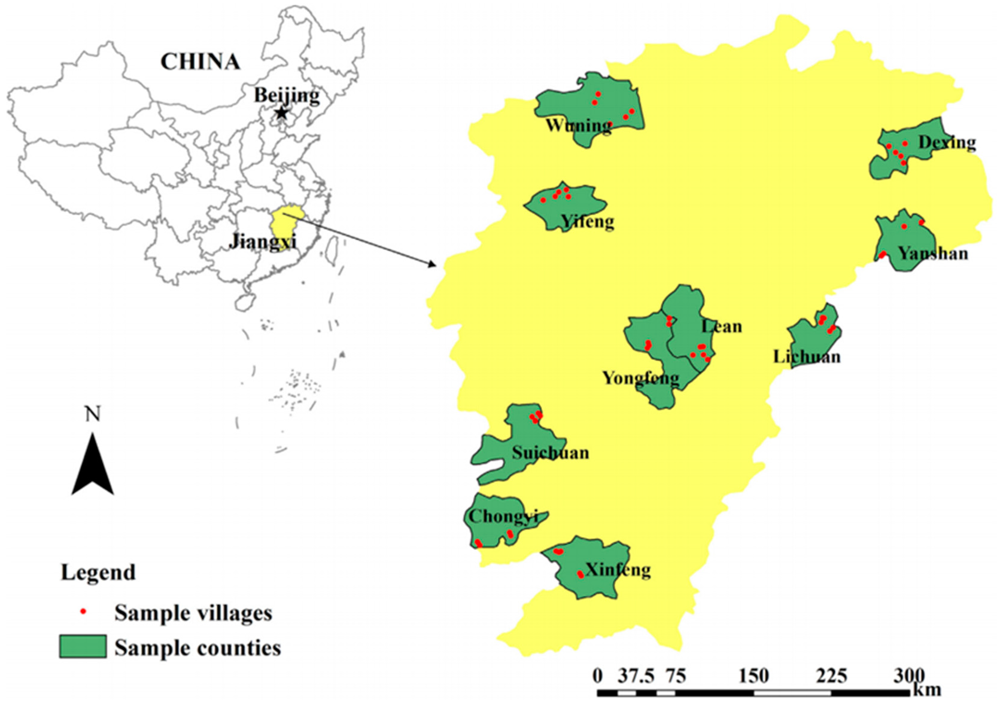
3.1. Data Sources
3.2. Variable Selection
3.2.1. Dependent Variables
3.2.2. Independent Variables
3.2.3. Control Variables
3.3. Descriptive Analysis
3.4. Model Construction
4. Empirical Analysis
4.1. Baseline Regression
4.2. Quantile Regression
4.3. Robustness Test
4.4. Heterogeneity Analysis
4.5. Endogeneity Test
5. Discussion
6. Conclusions and Policy Implications
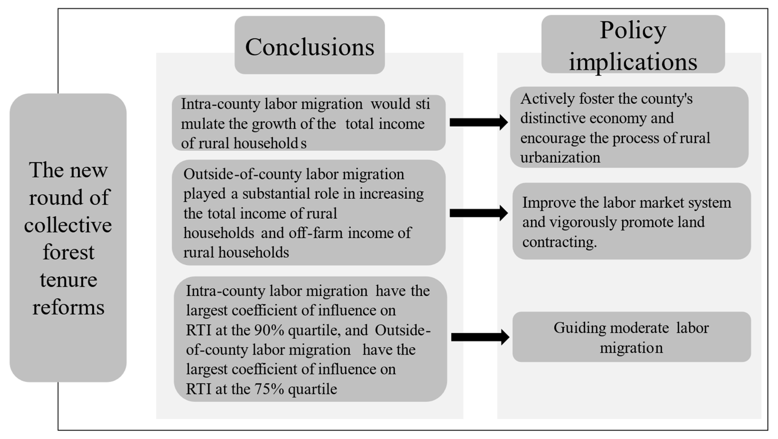
6.1. Conclusions
6.2. Policy Implications
Author Contributions
Funding
Informed Consent Statement
Data Availability Statement
Acknowledgments
Conflicts of Interest
References
- Gollin, D. The Lewis model: A 60-year retrospective. J. Econ. Perspect. 2014, 28, 71–88. [Google Scholar] [CrossRef]
- Montoya, A.C. Los Modelos Duales de Crecimiento y el Desarrollo Económico de México (1971–1984). 1987. Available online: https://www.proquest.com/openview/05418ebb5bac08f8c8cb8b6a85a6f8b0/1?pq-origsite=gscholar&cbl=18750&diss=y (accessed on 22 July 2024).
- Han, S. Specification and Estimation of an Alternative Neoclassical Investment Model. 1984. Available online: https://documents.worldbank.org/en/publication/documents-reports/documentdetail/416901468140979731/rural-urban-migration-in-developing-countries-a-survey-of-theoretical-predictions-and-empirical-findings?_gl=1*1q29urm*_gcl_au*MTUyNTAyODk4Ny4xNzI0NjQyODI1 (accessed on 22 July 2024).
- Espíndola, A.L.; Silveira, J.J.; Penna, T.J.P. A Harris-Todaro agent-based model to rural-urban migration. Braz. J. Phys. 2006, 36, 603–609. [Google Scholar] [CrossRef]
- Lall, S.V.; Selod, H. Rural-Urban Migration in Developing Countries: A Survey of Theoretical Predictions and Empirical Findings; World Bank Publications: Chicago, IL, USA, 2006; Volume 3915. [Google Scholar]
- Lagakos, D. Urban-rural gaps in the developing world: Does internal migration offer opportunities? J. Econ. Perspect. 2020, 34, 174–192. [Google Scholar] [CrossRef]
- Minale, L. Agricultural productivity shocks, labour reallocation and rural–urban migration in China. J. Econ. Geogr. 2018, 18, 795–821. [Google Scholar] [CrossRef]
- Huang, K.; Yan, W.; Huang, J. Agricultural subsidies retard urbanisation in China. Aust. J. Agric. Resour. Econ. 2020, 64, 1308–1327. [Google Scholar] [CrossRef]
- Luo, T.; Guan, Z. Public health insurance and migration of farm workers in the US. Appl. Econ. 2022, 54, 1672–1687. [Google Scholar] [CrossRef]
- D’Antoni, J.M.; Mishra, A.K.; Barkley, A.P. Feast or flee: Government payments and labor migration from US agriculture. J. Policy Model. 2012, 34, 181–192. [Google Scholar] [CrossRef]
- Lyu, H.; Dong, Z.; Roobavannan, M.; Kandasamy, J.; Pande, S. Prospects of interventions to alleviate rural–urban migration in Jiangsu Province, China based on sensitivity and scenario analysis. Hydrol. Sci. J. 2020, 65, 2175–2184. [Google Scholar] [CrossRef]
- Ramsey, A.F.; Sonoda, T.; Ko, M. Intersectoral labor migration and agriculture in the United States and Japan. Agric. Econ. 2023, 54, 364–381. [Google Scholar] [CrossRef]
- Ellis, F.; Freeman, H.A. Rural livelihoods and poverty reduction strategies in four African countries. J. Dev. Stud. 2004, 40, 1–30. [Google Scholar] [CrossRef]
- Qian, L.; Zhang, Z.M.; Li, N. Impact of migration on agricultural labor supply of left-behind farmers: An empirical analysis based on CFPS2012. J. China Agric. Univ. 2018, 23, 169–181. (In Chinese) [Google Scholar]
- Xu, D.; Deng, X.; Guo, S.; Liu, S. Labor migration and farmland abandonment in rural China: Empirical results and policy implications. J. Environ. Manag. 2019, 232, 738–750. [Google Scholar] [CrossRef] [PubMed]
- KARKI NEPAL, A.; Nepal, M.; Bluffstone, R. International labour migration, farmland fallowing, livelihood diversification and technology adoption in Nepal. Int. Labour Rev. 2023, 162, 687–713. [Google Scholar] [CrossRef]
- Wang, S.X.; Benjamin, F.Y. Labor mobility barriers and rural-urban migration in transitional China. China Econ. Rev. 2019, 53, 211–224. [Google Scholar] [CrossRef]
- Anang, B.T.; Nkrumah-Ennin, K.; Nyaaba, J.A. Does Off-Farm Work Improve Farm Income? Empirical Evidence from Tolon District in Northern Ghana. Adv. Agric. 2020, 2020, 1406594. [Google Scholar] [CrossRef]
- Babatunde, R.O. On-farm and Off-farm works: Complement or substitute? Evidence from Nigeria. Maastricht Sch. Manag. Work. Pap. 2015, 2, 1–41. [Google Scholar]
- Zhao, Y. Labor migration and earnings differences: The case of rural China. Econ. Dev. Cult. Chang. 1999, 47, 767–782. [Google Scholar] [CrossRef]
- Gao, J.; Song, G.; Sun, X. Does labor migration affect rural land transfer? Evidence from China. Land Use Policy 2020, 99, 105096. [Google Scholar] [CrossRef]
- Ning, C.; Xie, F.; Xiao, H.; Rao, P.; Zhu, S. Impact and mechanism of rural labor migration on forest management income: Evidence from the Jiangxi Province, China. Front. Environ. Sci. 2022, 10, 902153. [Google Scholar] [CrossRef]
- Nguyen, D.L.; Grote, U.; Nguyen, T.T. Migration, crop production and non-farm labor diversification in rural Vietnam. Econ. Anal. Policy 2019, 63, 175–187. [Google Scholar] [CrossRef]
- Gisbert, M.; Painter, M.; Quiton, M. Gender issues associated with labor migration and dependence on off-farm income in rural Bolivia. Hum. Organ. 1994, 53, 110–122. [Google Scholar] [CrossRef]
- Wan, J.; Li, R.; Wang, W.; Liu, Z.; Chen, B. Income diversification: A strategy for rural region risk management. Sustainability 2016, 8, 1064. [Google Scholar] [CrossRef]
- Reardon, T.; Crawford, E.; Kelly, V. Links between nonfarm income and farm investment in African households: Adding the capital market perspective. Am. J. Agric. Econ. 1994, 76, 1172–1176. [Google Scholar] [CrossRef]
- Foster, A.D.; Rosenzweig, M.R. Are Indian Farms too Small? Mechanization, Agency Costs, and Farm Efficiency. Brown University and Yale University. 2011; Unpublished Manuscript. [Google Scholar]
- Wang, X.; Yamauchi, F.; Huang, J. Rising wages, mechanization, and the substitution between capital and labor: Evidence from small scale farm system in China. Agric. Econ. 2016, 47, 309–317. [Google Scholar] [CrossRef]
- Atchoarena, D.; Wallace, I.; Green, K.; Gomes, C.A. Strategies and institutions for promoting skills for rural development. Educ. Rural Dev. New Policy Responses 2003, 239. [Google Scholar]
- Fafchamps, M.; Quisumbing, A.R. Human capital, productivity, and labor allocation in rural Pakistan. J. Hum. Resour. 1999, 34, 369–406. [Google Scholar] [CrossRef]
- Guang, L.; Zheng, L. Migration as the second-best option: Local power and off-farm employment. China Q. 2005, 181, 22–45. [Google Scholar] [CrossRef]
- Li, L.; Khan, S.U.; Guo, C.; Huang, Y.; Xia, X. Non-agricultural labor transfer, factor allocation and farmland yield: Evidence from the part-time peasants in Loess Plateau region of Northwest China. Land Use Policy 2022, 120, 106289. [Google Scholar] [CrossRef]
- Xu, D.; Guo, S.; Xie, F.; Liu, S.; Cao, S. The impact of rural laborer migration and household structure on household land use arrangements in mountainous areas of Sichuan Province, China. Habitat Int. 2017, 70, 72–80. [Google Scholar] [CrossRef]
- Barbier, E.B.; Burgess, J.C. Tropical deforestation, tenure insecurity, and unsustainability. For. Sci. 2001, 47, 497–509. [Google Scholar] [CrossRef]
- Zhou, Y.; Shi, X.; Ji, D.; Ma, X.; Chand, S. Property rights integrity, tenure security and forestland rental market participation: Evidence from Jiangxi Province, China. In Natural Resources Forum; Blackwell Publishing Ltd.: Oxford, UK, May 2019; Volume 43, pp. 95–110. [Google Scholar]
- Ma, E.; Liu, A.; Li, X.; Wu, F.; Zhan, J. Impacts of Vegetation Change on the Regional Surface Climate: A Scenario-Based Analysis of Afforestation in Jiangxi Province, China. Adv. Meteorol. 2013, 2013, 796163. [Google Scholar] [CrossRef]
- Xie, F.; Zhu, S.; Cao, M.; Kang, X.; Du, J. Does rural labor outward migration reduce household forest investment? The experience of Jiangxi, China. For. Policy Econ. 2019, 101, 62–69. [Google Scholar] [CrossRef]
- Ma, W.; Zhou, X.; Renwick, A. Impact of off-farm income on household energy expenditures in China: Implications for rural energy transition. Energy Policy 2019, 127, 248–258. [Google Scholar] [CrossRef]
- Liu, S.; Xie, F.; Zhang, H.; Guo, S. Influences on rural migrant workers’ selection of employment location in the mountainous and upland areas of Sichuan, China. J. Rural Stud. 2014, 33, 71–81. [Google Scholar] [CrossRef]
- Xiao, H.; Ning, C.; Xie, F.; Kang, X.; Zhu, S. Influence of rural labor migration behavior on the transfer of forestland. Nat. Resour. Model. 2021, 34, e12293. [Google Scholar] [CrossRef]
- Chen, Z.; Sarkar, A.; Hossain, M.S.; Li, X.; Xia, X. Household Labour Migration and Farmers’ Access to Productive Agricultural Services: A Case Study from Chinese Provinces. Agriculture 2021, 11, 976. [Google Scholar] [CrossRef]
- Yang, Y.; Li, H.; Liu, Z.; Cheng, L.; Abu Hatab, A.; Lan, J. Effect of forestland property rights and village off-farm environment on off-Farm employment in Southern China. Sustainability 2020, 12, 2605. [Google Scholar] [CrossRef]
- Liu, G.; Wang, H.; Cheng, Y.; Zheng, B.; Lu, Z. The impact of rural out-migration on arable land use intensity: Evidence from mountain areas in Guangdong, China. Land Use Policy 2016, 59, 569–579. [Google Scholar] [CrossRef]
- Koenker, R.; Bassett, G., Jr. Regression quantiles. Econom. J. Econom. Soc. 1978, 33–50. [Google Scholar] [CrossRef]
- Yu, H.; Zhan, Z.; He, Y.; Cheng, Y. Impact of rural labor migration on rural household income and rural-urban inequality in China. In Proceedings of the 2021 3rd International Conference on E-Business and E-commerce Engineering, Sanya, China, 17–19 December 2021; pp. 164–169. [Google Scholar]
- Oaxaca, R. Male-female wage differentials in urban labor markets. Int. Econ. Rev. 1973, 14, 693–709. [Google Scholar] [CrossRef]
- Pedraza, S. Women and migration: The social consequences of gender. Annu. Rev. Sociol. 1991, 303–325. [Google Scholar] [CrossRef] [PubMed]
- Ma, Z.; Ran, R.; Xu, D. The Effect of Peasants Differentiation on Peasants’ Willingness and Behavior Transformation of Land Transfer: Evidence from Sichuan Province, China. Land 2023, 12, 338. [Google Scholar] [CrossRef]
- Ji, X.; Qian, Z.; Zhang, L.; Zhang, T. Rural labor migration and Households’ land rental behavior: Evidence from China. China World Econ. 2018, 26, 66–85. [Google Scholar] [CrossRef]
- Meng, X.; Zhang, J. The two-tier labor market in urban China: Occupational segregation and wage differentials between urban residents and rural migrants in Shanghai. J. Comp. Econ. 2001, 29, 485–504. [Google Scholar] [CrossRef]
- Li, S. Effects of labor out-migration and income growth and inequality in rural China. In China’s Economy: Rural Reform and Agricultural Development; World Scientific: Singapore, 2009; pp. 161–185. Available online: https://www.worldscientific.com/doi/abs/10.1142/9789814293327_0005 (accessed on 22 July 2024).


| Variable | Variable Symbol | Definition | Mean | SD |
|---|---|---|---|---|
| Dependent variable | ||||
| Total rural households’ income | RTI (ln) | RTI (including income from forestry activities, off-farm employment, agricultural activities, and others) (Yuan) in 2018 taken in logarithms | 11.027 | 1.458 |
| Rural households’ forestry income | RFI (ln) | RFI (including income from timber forests, bamboo forests, economic forests, under-forest economy, the income from forest-related part-time employment, and other income) (Yuan) in 2018 taken in logarithms | 5.682 | 4.208 |
| Rural households’ off-farmer income | ROI (ln) | ROI (including off-farm income in this study is defined as off-farm income, wages, salaries, and remittances of household members) (Yuan) in 2018 taken in logarithms | 10.660 | 1.983 |
| Independent variable | ||||
| Intra-county labor migration | Number of intra-county labor migration/Number of family laborers (%) | 0.223 | 0.342 | |
| Outside-of-county labor migration | Number of outside-of-county labor migration/Number of family laborers (%) | 0.310 | 0.360 | |
| Control variables | ||||
| Personal characteristics of the head of household | ||||
| Age | Age of head of household in the year of survey (actual years) | 56.805 | 10.185 | |
| Educational level | Educational level of the head of household (elementary school and below = 1; middle school = 2; middle or high school = 3; college or bachelor’s degree or higher = 4 | 1.899 | 0.823 | |
| Whether village cadres | Whether the head of household is a village cadre (Yes = 1; No = 0) | 0.392 | 0.500 | |
| Family characteristics | ||||
| Number of family members | Number of family (persons) | 4.824 | 2.228 | |
| Whether or not there is labor migration? | Whether or not there is labor migration in the rural household (Yes = 1; No = 0) | 0.640 | 0.480 | |
| Number of laborers | Number of family laborers (persons) | 2.842 | 1.427 | |
| Number of outgoing laborers | Number of outgoing laborers (persons) | 1.239 | 1.260 | |
| Village Characteristics | ||||
| Area of forestland | Total area of forestland (hectares) | 8.044 | 20.325 | |
| Average area of forestland | Total area of forestland/number of forested plots (hectares) | 1.670 | 3.066 | |
| Distance | Distance from the village to the town center (kilometers) | 7.242 | 6.058 | |
| Percentage of village labor migration | Number of village labor migration/total number of villages | 0.497 | 0.204 | |
| Village income | Village income (including financial assistance income, resource exploitation and remittance income, management income, investment income, and other income) (Yuan) in 2018 taken in logarithms | 8.618 | 0.311 | |
| Village population | Village population(person) logarithmic for the year before the year of household research | 7.119 | 0.699 |
| Variables | Dependent Variable: RTI (ln) | Dependent Variable: RFI (ln) | Dependent Variable: ROI (ln) | |||
|---|---|---|---|---|---|---|
| Model 1 | Model 2 | Model 3 | Model 4 | Model 5 | Model 6 | |
| 0.255 ** (0.190) | 0.285 ** (0.172) | 0.888 (0.547) | 0.539 (0.527) | 0.266 (0.258) | 0.140 (0.240) | |
| — | −0.021 *** (0.006) | — | 0.005 (0.019) | — | −0.027 *** (0.009) | |
| — | 0.085 (0.079) | — | 0.112 (0.243) | — | 0.163 (0.111) | |
| — | 0.154 (0.122) | — | −0.550 (0.376) | — | 0.343 ** (0.171) | |
| — | −0.016 (0.027) | — | −0.067 (0.083) | — | −0.010 (0.038) | |
| — | −0.057 (0.182) | — | 0.237 (0.559) | — | 0.184 (0.255) | |
| — | 0.249 *** (0.057) | — | 0.667 *** (0.174) | — | 0.218 *** (0.079) | |
| — | 0.190 ** (0.083) | — | −0.699 *** (0.255) | — | 0.292 ** (0.116) | |
| — | 0.006 (0.006) | — | 0.024 (0.017) | — | 0.001 (0.008) | |
| — | 0.032 (0.038) | — | 0.148 (0.116) | — | −0.154 *** (0.053) | |
| — | −0.004 (0.011) | — | −0.053 (0.033) | — | 0.000 (0.015) | |
| — | −0.240 (0.334) | — | −2.711 *** (1.024) | — | 0.183 (0.466) | |
| — | 0.743 *** (0.199) | — | −0.134 (0.610) | — | 0.886 *** (0.277) | |
| — | 0.355 *** (0.087) | — | −0.470 * (0.266) | — | 0.378 *** (0.121) | |
| Cons | 10.970 *** (0.077) | 2.300 (1.902) | 5.484 *** (0.223) | 10.230 * (5.839) | 10.600 *** (0.105) | 0.420 (2.657) |
| N | 506 | 506 | 506 | 506 | 506 | 506 |
| Adj R2 | 0.002 | 0.237 | 0.003 | 0.126 | 0.000 | 0.197 |
| Variables | Dependent Variable: RTI (ln) | Dependent Variable: RFI (ln) | Dependent Variable: ROI (ln) | |||
|---|---|---|---|---|---|---|
| Model 7 | Model 8 | Model 9 | Model 10 | Model 11 | Model 12 | |
| 0.357 ** (0.180) | 0.345 ** (0.174) | −1.082 ** (0.518) | −0.547 ** (0.335) | 1.082 ** (0.518) | 0.052 (0.243) | |
| Control | — | Yes | — | Yes | — | Yes |
| Cons | 11.07 *** (0.086) | 2.241 (1.897) | 6.018 *** (0.246) | 9.944 * (5.835) | 6.018 *** (0.246) | 0.364 (2.656) |
| N | 506 | 506 | 506 | 506 | 506 | 506 |
| Adj R2 | −0.001 | 0.239 | 0.007 | 0.126 | 0.007 | 0.196 |
| Variables | Dependent Variable: RTI (ln) | Dependent Variable: RFI (ln) | ||||||
|---|---|---|---|---|---|---|---|---|
| 25% | 50% | 75% | 90% | 25% | 50% | 75% | 90% | |
| Model 13 | Model 14 | Model 15 | Model 16 | Model 17 | Model 18 | Model 19 | Model 20 | |
| 0.019 (0.140) | 0.162 (0.130) | 0.229 * (0.181) | 0.341 ** (0.181) | 0.911 (1.327) | 0.866 (0.719) | −0.173 (0.399) | −0.131 (0.507) | |
| 0.003 (0.168) | 0.250 * (0.161) | 0.980 ** (0.452) | 0.461 ** (0.228) | 0.061 (1.028) | 0.002 (0.748) | −0.601 (0.467) | −0.898 ** (0.424) | |
| Control | Yes | Yes | Yes | Yes | Yes | Yes | Yes | Yes |
| Cons | 5.132 *** (1.437) | 5.280 *** (1.447) | 4.373 ** (1.854) | 4.693 (3.527) | 16.130 (12.770) | 9.025 (9.098) | 5.143 (4.630) | −0.248 (5.112) |
| N | 506 | 506 | 506 | 506 | 506 | 506 | 506 | 506 |
| R2 | 0.242 | 0.214 | 0.201 | 0.220 | 0.044 | 0.093 | 0.108 | 0.137 |
| Variables | Dependent Variable: RTI (ln) | Dependent Variable: RFI (ln) | Dependent Variable: ROI (ln) | Dependent Variable: RTI (ln) | Dependent Variable: RFI (ln) | Dependent Variable: ROI (ln) |
|---|---|---|---|---|---|---|
| Model 21 | Model 22 | Model 23 | Model 24 | Model 25 | Model 26 | |
| 0.364 ** (0.159) | 0.427 (0.583) | 0.153 (0.265) | 0.314 * (0.216) | 0.272 (0.286) | −0.152 (0.297) | |
| 0.282 ** (0.132) | −0.596 ** (0.461) | 0.145 (0.271) | 0.327 * (0.157) | −0.433 * (0.304) | 0.296 (0.310) | |
| Control | Yes | Yes | Yes | Yes | Yes | Yes |
| Cons | 4.632 *** (1.302) | 10.830 * (5.892) | −0.364 (2.681) | 13.040 *** (3.097) | 0.919 (2.864) | 9.201 *** (3.038) |
| N | 506 | 506 | 506 | 506 | 506 | 506 |
| Adj R2 | 0.293 | 0.178 | 0.178 | 0.199 | 0.200 | 0.199 |
| Variables | Dependent Variable: RTI (ln) | Dependent Variable: RFI (ln) | ||||
|---|---|---|---|---|---|---|
| Scale = 1 | Scale = 2 | Scale = 3 | Scale = 1 | Scale = 2 | Scale = 3 | |
| Model 27 | Model 28 | Model 29 | Model 30 | Model 31 | Model 32 | |
| Laborin | 0.433 (0.308) | 0.473 ** (0.382) | 0.342 ** (0.198) | −0.414 (1.027) | 1.309 (0.957) | −1.008 (1.070) |
| Laborout | 0.997 ** (0.571) | 0.581 * (0.411) | 0.532 ** (0.359) | 0.263 (0.903) | 1.372 (1.030) | −2.497 ** (1.123) |
| Control | Yes | Yes | Yes | Yes | Yes | Yes |
| Cons | −2.436 (3.889) | −0.726 (4.355) | 6.600 ** (2.818) | 10.100 (12.980) | −9.495 (10.910) | 15.380 * (8.815) |
| N | 166 | 171 | 169 | 166 | 171 | 169 |
| R2 | 0.307 | 0.150 | 0.155 | 0.162 | 0.175 | 0.173 |
| Variables | Dependent Variable: RTI (ln) | Dependent Variable: RFI (ln) | ||
|---|---|---|---|---|
| = 0 | = 1 | = 0 | = 1 | |
| Model 33 | Model 34 | Model 35 | Model 36 | |
| 0.228 ** (0.121) | 0.354 ** (0.147) | 0.002 (0.695) | 1.018 (1.187) | |
| 0.431 ** (0.234) | 0.126 (0.335) | −0.494 (0.712) | −1.184 ** (0.725) | |
| Control | Yes | Yes | Yes | Yes |
| Cons | 3.306 (2.301) | −2.515 (3.576) | 7.676 (7.012) | 2.160 (12.00) |
| N | 364 | 142 | 364 | 142 |
| R2 | 0.172 | 0.184 | 0.198 | 0.093 |
| Variables | Dependent Variable: RTI (ln) | Dependent Variable: RFI (ln) | Dependent Variable: ROI (ln) | Dependent Variable: RTI (ln) | Dependent Variable: RFI (ln) | Dependent Variable: ROI (ln) |
|---|---|---|---|---|---|---|
| Model 37 | Model 38 | Model 39 | Model 40 | Model 41 | Model 42 | |
| 0.327 ** (0.192) | 0.371 (0.591) | 0.205 (0.269) | 0.267 * (0.171) | 0.135 (0.434) | 0.153 (0.123) | |
| 0.662 ** (0.310) | 0.742 (0.150) | 8.842 (15.540) | 0.432 ** (0.249) | 0.120 (0.978) | 0.343 (0.278) | |
| Control | Yes | Yes | Yes | Yes | Yes | Yes |
| −9.929 (11.110) | −1.121 (34.170) | −8.704 (15.550) | — | — | — | |
| Cons | −0.613 (3.701) | 9.803 (11.390) | −2.026 (5.180) | 5.045 (5.172) | 5.394 (289.700) | 0.142 (0.826) |
| N | 506 | 506 | 506 | 506 | 506 | 506 |
| R2 | 0.126 | 0.121 | 0.107 | 0.093 | 0.086 | 0.042 |
Disclaimer/Publisher’s Note: The statements, opinions and data contained in all publications are solely those of the individual author(s) and contributor(s) and not of MDPI and/or the editor(s). MDPI and/or the editor(s) disclaim responsibility for any injury to people or property resulting from any ideas, methods, instructions or products referred to in the content. |
© 2024 by the authors. Licensee MDPI, Basel, Switzerland. This article is an open access article distributed under the terms and conditions of the Creative Commons Attribution (CC BY) license (https://creativecommons.org/licenses/by/4.0/).
Share and Cite
Li, L.; Luo, X.; Liu, Y.; Liu, Y.; Liu, X. The Impact of Location of Labor Migration on Rural Households’ Income: Evidence from Jiangxi Province in China. Agriculture 2024, 14, 1458. https://doi.org/10.3390/agriculture14091458
Li L, Luo X, Liu Y, Liu Y, Liu X. The Impact of Location of Labor Migration on Rural Households’ Income: Evidence from Jiangxi Province in China. Agriculture. 2024; 14(9):1458. https://doi.org/10.3390/agriculture14091458
Chicago/Turabian StyleLi, Lishan, Xin Luo, Yanshan Liu, Yuan Liu, and Xiaojin Liu. 2024. "The Impact of Location of Labor Migration on Rural Households’ Income: Evidence from Jiangxi Province in China" Agriculture 14, no. 9: 1458. https://doi.org/10.3390/agriculture14091458