A Highland Barley Crop Extraction Method Based on Optimized Feature Combination of Multiple Phenological Sentinel-2 Images

Abstract

Previous studies have primarily focused on the extraction of highland barley crops using single phenological images, which ignored the selection of the optimal phenological period for classification. Utilizing the multiple phenological images from Sentinel-2 to construct 25 features, including spectral, red edge, vegetation, and texture features, the recursive feature elimination algorithm and the random forest algorithm (RF) were employed to optimize feature datasets for different phenological stages, which were then used for the identification and classification of high-land barley by RF. The main results were as follows: (1) Information extraction based on feature optimization combinations yielded good overall classification accuracy, with classification accuracies for highland barley being 92.56% (jointing stage), 90.90% (heading stage), 90.74% (flowering stage), 91.55% (milk ripening stage), and 90.51% (maturity stage), respectively. (2) NDVIre1 had the highest importance score (0.1792) in the feature selection combination, indicating that the red edge index contributed significantly to crop information extraction and classification. (3) The five feature variables—GLCM_Mean, RVI, homogeneity, MAX, and GLCM_Correlation—showed stability and universality in the extraction of highland barley. These results demonstrated that the images that derived from the jointing and milk ripening phenological stages had the best applicability for highland barley extraction, and the optimized feature datasets that composed of NDVIre1 were conductive to detect and monitor of highland barley crops in the mountainous regions of northwest China.

1. Introduction

Crop classification and extraction constitute a fundamental data basis for the adjustment of agricultural planting structures. They are also of great importance for the assessment and prediction of food production, which is conducive to agricultural and crop management. There are numerous methods for extracting crops. The traditional method of crop classification relies on biological and morphological investigation, which is an accurate method but requires significant financial and material resources. This is not aligned with the current situation of the development of efficient monitoring technology in society. The current mainstream trend is the use of remote sensing technology to monitor crops [1].

Satellite remote sensing technology enables the real-time and long-term ground observation of crops over large areas, facilitating the acquisition of accurate information on their distribution. Currently, scholars employ UAV technology to monitor crops, and the advantages of UAV hyperspectral remote sensing image technology lie in its characteristics of large numbers of bands and long wavelengths, as well as the large amounts of information it can provide [2]. Liang et al. [3] employed the support vector machine (SVM) classification method and the random forest (RF) method to categorize soybean, corn, and other crops based on UAV hyperspectral remote sensing images. Their study indicated that the RF classification method was more effective in classifying crops based on hyperspectral images. However, in the classification process, they did not consider selecting classification features that were suitable for the crops. Zhang et al. [4] utilized a random forest (RF) model to classify crops based on unmanned aerial vehicle (UAV) images and then evaluated the accuracy of crops, which provided technical support and theoretical references for crop extraction in small-scale crop-growing areas. However, validating the accuracy of each method using only single-temporal imagery failed to capture the full range of seasonal and phenological changes, which may affect the robustness and generalizability of their results. Cheng et al. [5] extracted sugarcane based on time series NDVI and verified the separability of the target crop from other land cover types using decision tree classification. However, the decision tree classification method used had low accuracy. Bao et al. [6] obtained the preferred combination of crop features based on GF-6 images using the RF algorithm, which demonstrated that the object-oriented method of feature preference was an effective means of improving classification accuracy. In this classification study, the failure to consider selecting the phenological period of the crops may have resulted in classification outcomes that did not accurately reflect the characteristics of crops at different growth stages, thereby affecting the accuracy and effectiveness of the classification. Yan et al. [7] applied Landsat and MODIS NDVI-based NDVI to classify sugarcane, which effectively mitigated the impact of heterogeneity within the same object and represented a more cost-effective approach than traditional methods. However, the classification accuracy was not high when they used Landsat as the data source. Liu et al. [8] employed a multiscale segmentation approach coupled with an object-oriented classification methodology to delineate the spatial planting structures of soybean and rice in Huainan County, which indicated that the proposed methodology could serve as an efficacious means for the extraction and monitoring of the county’s crops. However, they also only used single-temporal imagery to validate the accuracy of each method. Xie et al. [9] leveraged Sentinel-1 data to investigate the impact of various environmental factors on the growth and development of winter wheat. The utilization of Google Earth Engine (GEE) and the RF algorithm enabled the analysis of the importance of multiclass feature variables, the identification of feature-preferred combinations, and the exploration of the influence of feature-preferred combinations on the extraction effect of winter wheat, which provided important theoretical references for the study of crop-planting area extraction based on multisource optical and radar remote sensing images. Shi et al. [10] employed HJ CCD and Landsat 8OLI image data to extract NDVI time series data of crops in their study area. Additionally, they selected five spectral feature variables and NDVI time series data to form a multisource dataset, which was used to categorize crops such as highland barley and wheat. They also did not consider selecting classification features that were suitable for the crops. Faqe et al. [11] demonstrated the efficacy of a novel approach for crop classification using integrated Sentinel-1 and Sentinel-2 data, which proved to be an invaluable tool for enhancing the accuracy of crop classification, particularly in the case of highland barley and wheat. They also only used single-temporal imagery to validate the accuracy of each method. Therefore, in crop identification and extraction studies, integrating multitemporal imagery to select suitable classification features is of significant importance [12]. Using the recursive feature elimination and random forest algorithms allows for the optimization of feature variables from multitemporal imagery. Optimal feature combinations can effectively reduce redundancy among feature variables while maintaining classification accuracy and efficiency. However, the optimal identification of different crops exhibits a significant disparity across seasonal periods. Therefore, it is necessary to conduct further research into the optimal classification period for highland barley and the optimal classification feature subset.

This study selected Sentinel-2 remote sensing imagery as the data source. Based on the recursive feature elimination and random forest algorithms, feature selection was performed on multitemporal imagery to obtain optimal feature combinations for each time period. Subsequently, the random forest classification method was employed, using these optimal feature combinations, to identify and extract highland barley. The aim was to determine the optimal phenological period for highland barley and identify the most effective subset of feature variables for highland barley extraction, thereby providing theoretical support and scientific guidance for research on highland barley extraction.

2. Materials and Methods

2.1. Study Area

The Chengbei District is located in the northwest of Xining City, which is in the Qinghai Province of China. Its longitude is 101° 77′ E and its latitude is 36° 67′ N (Figure 1). It is situated to the east of the city junction, to the west of Huangshuzhong District, to the south of the city district, to the west of the Huangshui River, and to the north of the Datong Hui-Tuzu Autonomous County and the mutual aid Autonomous County of Tu. The climate within the territory is typified by low air pressure, low rainfall, evaporation, a long freezing period, a short frost-free period, and a significant temperature difference between day and night. The total area of Chengbei District is 129.3 square kilometers, of which 87,726 acres are designated as agricultural arable land, representing 42% of the total area. Additionally, there are 50,100 acres of forested land, comprising 25.6% of the total area. Furthermore, 16,374 acres of grassland are present, accounting for 7.9% of the total area. The remaining 8.71% of the total area comprises land that is currently unavailable for use, including roads, homes, and so forth. The terrain exhibits a high elevation in the northern region and a low elevation in the southeastern region. It slopes gently from west to east, exhibiting an inverted “herringbone” pattern. The elevation ranges from 2400 to 2750 meters above sea level at the northeastern and southwestern edges of the mountains within the territory.

2.2. Data Source and Preprocessing

Sentinel-2 images (

Table 1. Band information of the Sentinel-2 remote sensing images.

Bands	Central Wavelength (nm)	Bandwidth (nm)	Resolution (m)
B1: Coast/aerosol band	443	20	60
B2: Blue band	490	65	10
B3: Green band	560	35	10
B4: Red band	665	30	10
B5: Vegetation red edge (band 1)	705	15	20
B6: Vegetation red edge (band 2)	740	15	20
B7: Vegetation red edge (band 3)	783	20	20
B8: Near-infrared band (wide)	842	115	10
B8A: Near-infrared band (narrow)	865	20	20
B9: Water vapor band	945	20	60
B10: Cirrus band	1375	20	60
B11: Short-wave infrared (band 1)	1610	90	20
B12: Short-wave infrared (band 2)	2190	180	20

presents an overview of its various bands) were selected to encompass the entirety of the crop growth cycle, spanning from 16 June 2020 to 25 August 2020. The phenological periods of highland barley are presented in

Table 2. The corresponding phenological periods of highland barley at different times.

Image Date	0616	0706	0726	0811	0825
Phenological period of highland barley	Jointing stage	Heading stage	Flowering stage	Milk ripening stage	Maturity stage

. Sentinel-2 images have lots of advantages, including high spatial and temporal resolution and the red edge feature [13], which is crucial for crop classification and recognition. The requisite Sentinel-2 data were downloaded from ESA and the Level-2A product was selected, which contained 12 spectral bands. The irrelevant bands of the coastal/aerosol band (B1) were uniformly excluded. The Sentinel-2 Level-2A Atmospheric Correction Processor (Sen2cor) was employed in SNAP software for atmospheric correction [14], in conjunction with resampling to achieve spatial resolutions of 20 m and 60 m, with the aim of achieving a resolution of 10 m. Furthermore, preprocessing techniques, such as band fusion and cropping, were applied to the resampled data.

2.3. Sample Data

This study conducted field surveys in the Chengbei District using drone technology and field observations to obtain empirical data. Training and validation samples were then constructed using the collected dataset. The objective was to obtain information on feature samples, crop types, and the geographic locations of highland barley and other crops. This was accomplished by combining the results from our surveys with Google Earth images of the validation samples. The land cover types were then categorized into five categories: Urban, river, highland barley, other crops, and mountainous. The total number of samples was 1473, comprising 246 urban samples, 127 river samples, 984 highland barley samples, 108 other crop samples, and 8 mountainous samples. In this study, the sample data were randomly divided into training and validation samples in a ratio of 7:3.

2.4. Methods

The specific process of extracting highland barley in the northern part of the city based on the random forest algorithm is depicted in Figure 2. The Sentinel-2 image data were downloaded from ESA (https://scihub.copernicus.eu/dhus/#/home, accessed on 25 November 2023). The spectral features, texture features, vegetation features, water features, and red edge index features were extracted. Principal component analysis was employed to optimize the spectral features. A sample training set and a validation set were constructed based on the field sampling data. The random forest algorithm was used to construct the preferred combinations of feature variables. The preferred feature combinations of five temporal phases were then compared and analyzed. The benefits of extracting crops based on the preferred combinations of features from the Sentinel-2 data were explored.

2.4.1. Feature Set Construction

A total of 33 features, including spectral features, texture features, vegetation features, water features, and red edge index features, were selected for each time phase to construct a dataset (

Table 3. Crop information extraction and classification feature variables.

Characteristic Variable Set	Characteristic Variable	Explanation/Calculation Formula	Main References
Spectral Signature	Band	B2, B3, B4, B5, B6, B7, B8, B8A, B11, B12	--
Texture Features	Angular Second Moment (ASM)	${\displaystyle \sum _{\mathrm{i}}{\displaystyle \sum _{j}p{(i,j)}^2}}$	--
	Contrast	${\displaystyle \sum _{\mathrm{i}}{\displaystyle \sum _{j}p(i,j){(i-j)}^2}}$	--
	Dissimilarity	${\displaystyle \sum _{\mathrm{i}}{\displaystyle \sum _{j}p(i,j)\left|i-j\right|}}$	--
	Energy	${\displaystyle \sum _{\mathrm{i}}{\displaystyle \sum _{j}p{(i,j)}^2}}$	--
	Entropy	$-{\displaystyle \sum _{\mathrm{i}}{\displaystyle \sum _{j}p(i,j)\ln p(i,j)}}$	--
	Homogeneity	${\displaystyle \sum _{\mathrm{i}}{\displaystyle \sum _{j}p(i,j)}}{\displaystyle \frac{1}{1+{\left(i-j\right)}^2}}$	--
	MAX	$Max\{p(i,j)\}$	--
	GLCM_Correlation	${\displaystyle \sum _{\mathrm{i}}{\displaystyle \sum _j\frac{(i-Mean)(j-Mean)p{(i,j)}^2}{Variance}}}$	--
	GLCM_Mean	${\displaystyle \sum _{\mathrm{i}}{\displaystyle \sum _{j}p(i,j)i}}$	--
	GLCM_Variance	${\displaystyle \sum _{\mathrm{i}}{\displaystyle \sum _{j}p(i,j){(i-Mean)}^2}}$	--
Vegetation Index	Normalized Difference Vegetation Index (NDVI)	$\left({\mathrm{B}}_{8\mathrm{A}}-{\mathrm{B}}_4\right)/\left({\mathrm{B}}_{8\mathrm{A}}{+\mathrm{B}}_4\right)$	[15,16,17]
	Ratio Vegetation Index (RVI)	${\mathrm{B}}_{8\mathrm{A}}/{\mathrm{B}}_4$
	Difference Vegetation Index (DVI)	${\mathrm{B}}_{8\mathrm{A}}-{\mathrm{B}}_4$
	Modified Soil-Adjusted Vegetation Index (MSAVI)	${\displaystyle \frac{\left(2{\mathrm{B}}_{8\mathrm{A}}+1\right)-\sqrt{{\left(2{\mathrm{B}}_{8\mathrm{A}}+1\right)}^2-8\left({\mathrm{B}}_{8\mathrm{A}}-{\mathrm{B}}_4\right)}}{2}}$
	Soil-Adjusted Vegetation Index (SAVI)	$1.5\left({\mathrm{B}}_{8\mathrm{A}}-{\mathrm{B}}_4\right)/\left({\mathrm{B}}_{8\mathrm{A}}{+\mathrm{B}}_4+0.5\right)$
Water Index	Normalized Difference Water Index (NDWI)	$\left({\mathrm{B}}_3-{\mathrm{B}}_{8\mathrm{A}}\right)/\left({\mathrm{B}}_3{+\mathrm{B}}_{8\mathrm{A}}\right)$
	Modified Normalized Difference Water Index (MNDWI)	$\left({\mathrm{B}}_3-{\mathrm{B}}_{11}\right)/\left({\mathrm{B}}_3{+\mathrm{B}}_{11}\right)$
Red Edge Index	Red Edge Normalized Difference Vegetation Index (RNDVI)	$\left({\mathrm{B}}_5-{\mathrm{B}}_4\right)/\left({\mathrm{B}}_5{+\mathrm{B}}_4\right)$	[18]
	Red Edge Chlorophyll Index (CIre)	${\mathrm{B}}_{8\mathrm{A}}/{\mathrm{B}}_5-1$
	Modified Simple Ratio Red Edge Index (MSRre)	${\displaystyle \frac{{\mathrm{B}}_{8\mathrm{A}}/{\mathrm{B}}_5-1}{\sqrt{{\mathrm{B}}_{8\mathrm{A}}/{\mathrm{B}}_5+1}}}$
	Red Edge Normalized Difference Vegetation Index 1 (NDVIre1)	$\left({\mathrm{B}}_{8\mathrm{A}}-{\mathrm{B}}_5\right)/\left({\mathrm{B}}_{8\mathrm{A}}{+\mathrm{B}}_5\right)$
	Red Edge Normalized Difference Vegetation Index 2 (NDVIre2)	$\left({\mathrm{B}}_{8\mathrm{A}}-{\mathrm{B}}_6\right)/\left({\mathrm{B}}_{8\mathrm{A}}{+\mathrm{B}}_6\right)$
	Red Edge Normalized Difference Vegetation Index 3 (NDVIre3)	$\left({\mathrm{B}}_{8\mathrm{A}}-{\mathrm{B}}_7\right)/\left({\mathrm{B}}_{8\mathrm{A}}{+\mathrm{B}}_7\right)$
	Red Edge Normalized Difference 1 (NDre1)	$\left({\mathrm{B}}_6-{\mathrm{B}}_5\right)/\left({\mathrm{B}}_6{+\mathrm{B}}_5\right)$
	Red Edge Normalized Difference 2 (NDre2)	$\left({\mathrm{B}}_7-{\mathrm{B}}_5\right)/\left({\mathrm{B}}_7{+\mathrm{B}}_5\right)$

). A comparative analysis was conducted based on the time-phase feature sets of the five phenological phases. In this approach, the optimal spectral features were identified for inclusion in the spectral feature set of the 12 bands of the Sentinel-2 remote sensing images, which were determined using the principal component analysis method. However, it is important to note that there was a certain degree of information redundancy among the bands. By selecting the first three bands using the principal component analysis method, the information in the remaining bands could be fully characterized, thereby reducing the effect of band redundancy on classification accuracy.

2.4.2. Principal Component Analysis (PCA)

Principal component analysis (PCA) is a mathematical statistical method of dimensionality reduction [19], which was proposed by Bracais in 1846. In this study, PCA was used to extract spectral features from the set of feature variables. Orthogonal transformation was employed to transform the original random variables, the components of which were uncorrelated. This group of new random variables was referred to as the principal components [20]. PCA was employed to eliminate interactions between image bands, extract the principal spectral information expressed by multiple bands, reduce the workload of texture information extraction, remove the redundancy of spectral information expressed by multiple bands, achieve the purpose of spectral feature optimization, and improve work efficiency [21]. In this study, spectral features for each time period were extracted based on principal component analysis (PCA), with the extracted bands being Bands 2, 3, and 4 with their contribution rates being 78.5%, 10.8%, and 9.5% (taking the jointing stage as example), respectively (

Table 4. Principal component analysis (PCA) extraction results (jointing stage).

Principal Component Analysis	Contribution Rate
PCA_1	83.5%
PCA_2	9.8%
PCA_3	4.5%

).

2.4.3. GrayScale Covariance Matrix

The gray-level co-occurrence matrix (GLCM) is a statistical method that is used for texture analysis, which captures spatial structure and texture information within images. It was proposed by Haralick et al. in 1973 and is a method for calculating gray-level co-occurrence matrices of images. These matrices can then be used to derive second-order statistical features that describe the texture of the images. The GLCM has strong adaptive ability and robustness [22] and has been widely used with SAR, multispectral, high-resolution, and other images for texture extraction. The spatial recurrence of gray values in images gives rise to texture features. Texture is a phenomenon that is dependent upon the degree of effect and results from the spatial interaction of the tonal primitives that make up images [23]. The texture information included in images is derived from the neighboring pixels and plays a pivotal role in characterizing the objects or regions of interest identified within the images. The mathematical expression of this phenomenon is as follows:

$$P_{i,j}(d,Q)=\begin{array}{l}\#\{(x_1,y_1)(x_2,y_2)|f(x_1,y_1)=\\ i,f(x_2,y_2)=j,|(x_1,y_1)-(x_2,y_2)|=\\ d,L((x_1,y_1),(x_2,y_2))=\theta \}\end{array}$$

(1)

where $\#$ represents the number of elements in the set, $f(x_1,y_1)=i$ denotes the gray level of the pixel at position $\left(x_1,y_1\right)$ in the image as a function of $i$, $d=\{1,2,3,4\}$ denotes the distance between two pixels, and $\theta =\{0^{\mathrm{o}},{45}^{\mathrm{o}},{90}^{\mathrm{o}},{135}^{\mathrm{o}}\}$ denotes the direction angle between two pixels.

2.4.4. Random Forest Algorithm

The random forest (RF) algorithm is an algorithm that is based on the classification and regression tree (CART) algorithm, which was invented by Breiman et al. It generates multiple decision trees via integrated learning, which takes the decision tree as the basic unit and has high compatibility with multisource and multidimensional data [24,25]. The algorithm exhibits robust tolerance to missing values and outliers, which can help to rank the importance of feature variables. Its fundamental principle is to derive a sequence of classification accuracy models through rounds of training to construct a multiclassification model system $\{h_1(X),h_2(X),\cdots ,h_K(X)\}$ and obtain the final classification results through a simple majority voting decision. The equation is as follows:

$$H(x)=\arg \max {\displaystyle {\sum }_{i=1}^{K}I(h_i(x)=Y)}$$

(2)

where $H(x)$ is the combined classification model, $h_i(x)$ is the individual decision tree classification model, $Y$ is the output variable, and $I(h_i(x)=Y)$ is the representativeness function.

(1)

Construction, calibration, and variables of the random forest model

In this study, we used 70% of the total data as the training set, primarily for model training and parameter learning. Validation set: We used 20% of the data as the validation set, which was utilized for model tuning and hyperparameter selection. This subset helped us adjust parameters during training to prevent overfitting. Test set: The remaining 10% of the data was reserved for final model testing, ensuring that the model’s performance was accurately evaluated on completely independent samples. And during model construction, we systematically tuned the key parameters of the random forest using grid search combined with cross-validation. We experimented with different numbers of decision trees (e.g., 100, 200, 500) and selected the value that performed best on the validation set, and we limited the maximum depth of each tree to prevent overfitting, choosing a maximum depth of 10. We used cross-validation to calibrate the model, selecting hyperparameter combinations that performed consistently across different data splits to enhance the model’s generalization ability. In this study, the response variable was barley, which represents the target crop class we aimed to classify. Additionally, we selected various spectral and texture features (e.g., GLCM mean, RVI, homogeneity) as predictors, which were extracted from remote sensing data and used to predict the distribution of barley.

(2)

Crop information extraction and classification

The random forest classification process was as follows. The first step was the extraction of training samples, which was conducted by randomly combining the feature variables and then returning $N$ samples to form a training sample set. The second step was the construction of the random forest, which was conducted by forming a decision tree based on the training sample set and then establishing a random forest. In each decision tree at each node, $m$ feature variables were randomly extracted according to the principle of the smallest Gini coefficient, which was used to select the most capable classification of feature variables at a node for splitting. Finally, a random forest classifier was constructed based on the generated decision trees. The classifier was then used to classify the data and voting was applied to determine the category of the new sample [26]. To ensure the reliability of the data accuracy, the number of decision trees used in the random forest model for all periods was set to 100.

(3)

Importance discrimination of characteristic variables

The random forest algorithm is capable of not only accurately classifying remote sensing images but also ranking the relative importance of the feature variables involved in the classification process. This algorithm plays an essential role in feature optimization and dimensionality reduction. In this study, we calculated the importance scores of the feature variables based on the root mean square error of the out-of-bag (OOB) of the random forest algorithm [27]. The expression for this calculation is as follows:

$$V\left(X^j\right)={\displaystyle \frac{1}{N}}{\displaystyle {\sum }_{t=1}^n\left(e_t^j-e_t\right)}$$

(3)

where $n$ represents the number of decision trees in the random forest, $e_t$ denotes the out-of-bag error of a decision tree, $X^j$ signifies the randomly assigned value of the $j$ feature variable of the out-of-bag data, and $e_t^j$ is the out-of-bag error computed based on the new value of $X^j$. The change in $X^j$ resulted in an increase in the out-of-bag error, indicating that the variable $j$ played a pivotal role in the classification process.

2.4.5. Accuracy Assessment

In this study, a confusion matrix was used to validate the accuracy of the information extraction and classification results, as well as the simulation results of the PLUS model. A confusion matrix, also known as an error matrix, is mainly used to compare the degree of misclassification between classification results and actual values in accuracy assessment. We selected overall accuracy (OA), kappa coefficient, producer’s accuracy (PA), and user’s accuracy (UA) as evaluation metrics to assess various classification schemes and simulation results.

$$\mathrm{OA}={\displaystyle \frac{{\displaystyle {\sum }_{i=1}^k{N}_{ii}}}{N}}$$

(4)

$$\mathrm{Kappa}={\displaystyle \frac{N{\displaystyle {\sum }_{i=1}^k{N}_{ii}-{\displaystyle {\sum }_{i=1}^k{N}_{i+}{N}_{+i}}}}{N^2-{\displaystyle {\sum }_{i=1}^k{N}_{i+}{N}_{+i}}}}$$

(5)

$${\mathrm{PA}}_i={\displaystyle \frac{N_{ii}}{N_{+i}}}$$

(6)

$${\mathrm{UA}}_i={\displaystyle \frac{N_{ii}}{N_{i+}}}$$

(7)

where OA represents overall accuracy, which is used to describe the overall effectiveness of classification schemes or simulation results; kappa represents the kappa coefficient, which is used to express the consistency between classification or simulation results and actual values; PA_i and UA_i are the producer’s accuracy and user’s accuracy for the i-th land use type, respectively, and can be used to evaluate the quality of classification or simulation results for that land use type; N is the total number of samples; k is the total number of classes; N_ii is the number of correctly classified samples; and N_i+ and N_+i are the actual number of samples and the predicted number of samples for the i-th land use type, respectively.

3. Results

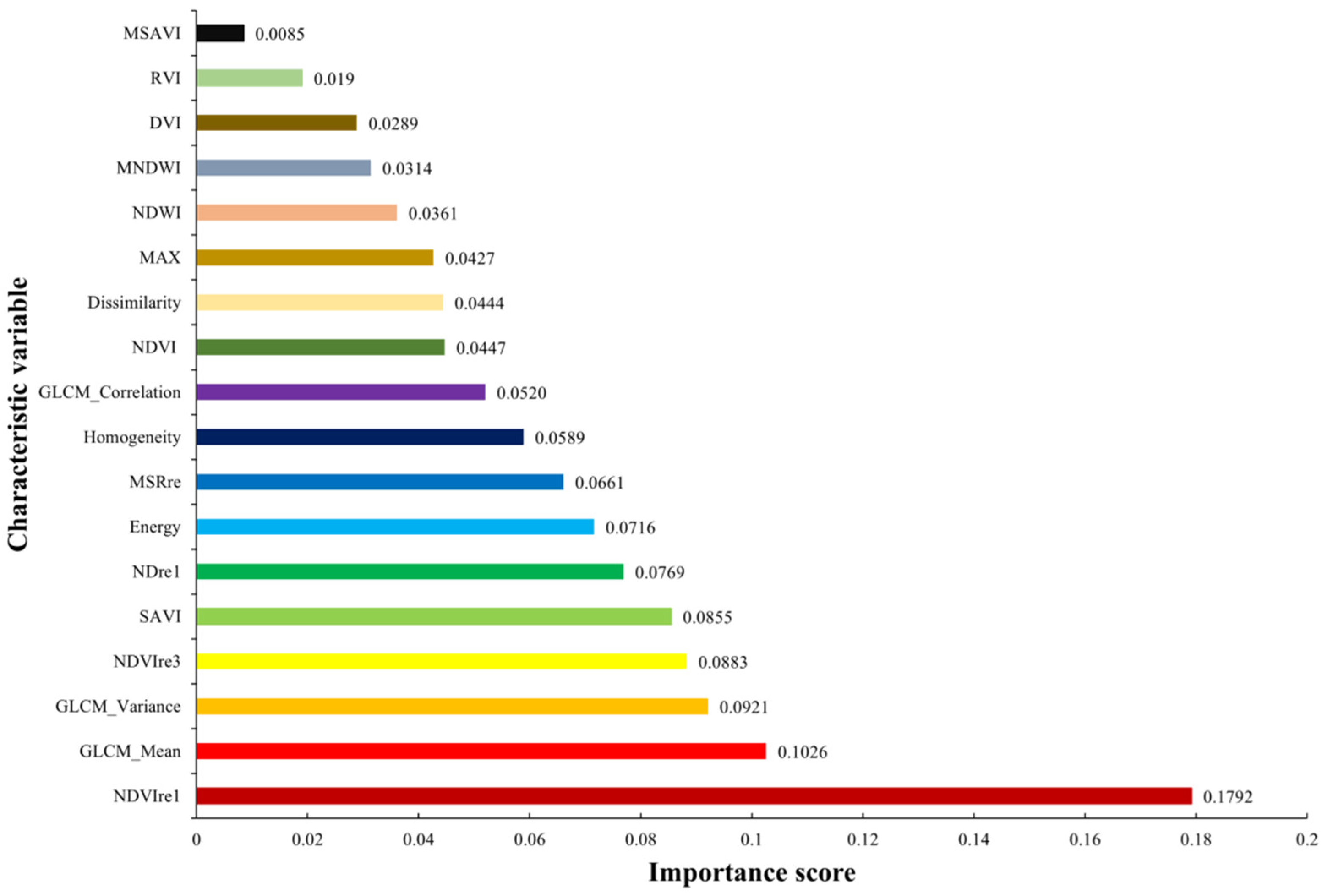
3.1. Importance Ranking of Characteristic Variables

As redundancy between different feature variables in the classification process increases model complexity and, thus, reduces classification accuracy, it was necessary to construct a preferred combination of feature variables [28]. In this study, 33 feature variables were selected for extraction, including five major feature sets: spectral features, texture features, vegetation features, the water body index, and the red edge index. The spectral feature set was constructed based on the principal component analysis method, which was applied to select the three main spectral bands. The recursive feature elimination method, based on the random forest algorithm, explored the relationship between the number of feature variables and the overall classification accuracy.

The Lasso regression model for training was used to rank the feature variables according to their feature weights. Feature variables with importance scores of 0 or below were eliminated, and the next round of training was carried out based on the new feature preference combinations. This process was repeated until the overall classification accuracy training ended, at which point the accuracy no longer improved. Based on the training results, a relationship graph between the feature variables and the overall classification accuracy (Figure 3) was obtained to explore the degree of correlation between the number of feature preferences and the classification accuracy.

Figure 3 indicates that when the number of feature variables was trained to 19, the classification accuracy reached a steady level and fluctuated around 95%. Furthermore, when the number of feature variables was reduced to 10, the overall classification accuracy began to show an obvious downward trend. The lowest overall classification accuracy was 71.56%, which was achieved when the number of feature variables was 4.

A random forest importance score analysis was performed on the extracted texture features, vegetation index, water body index, and red edge index (Figure 4). It was observed that the number of optimal feature preferences was not exactly the same in each period. This was due to the influence of weather conditions, such as cloudiness, on image quality. This, in turn, affected the machine recognition, and, thus, the optimal feature preferences were not exactly the same in each period. To illustrate, on 16 June 2020, the variable importance discrimination module in the random forest algorithm was employed to rank the importance of the texture features, vegetation index, water body index, and red edge index. This revealed that the feature variables of different regions exhibited varying degrees of importance in the process of crop extraction. For the highland barley crop, for instance, the feature variable NDVIre1 was identified as the most significant, with an importance score of 0.1792. This score had the greatest impact on the classification of crops. The northern part of the city was classified according to crops, with the results indicating that the red edge index was the most effective at extracting crop information. In contrast, the modified soil-adjusted vegetation index (MSAVI) had the lowest score, with minimal impact on crop classification in the northern part of the city. The feature preference combination, comprising 21 feature variables, exhibited the most favorable classification effect. The top 18 feature variables, ranked in order of importance, were selected to form the feature preference combination for each time phase, in conjunction with the top three spectral bands obtained from the principal component analysis method.

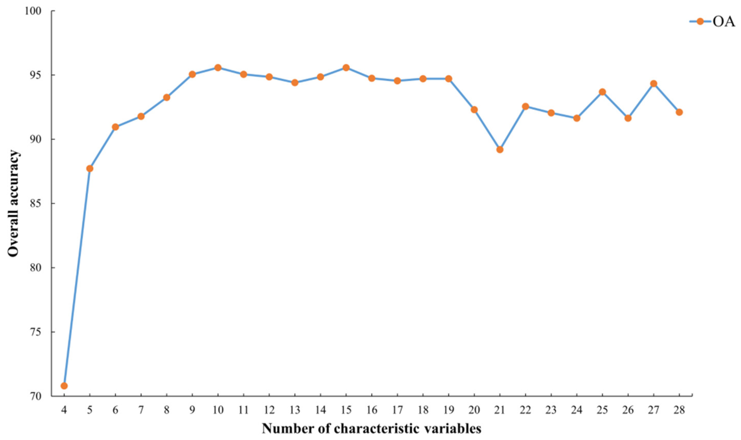
3.2. The Optimal Combination of Crop Classification Characteristics in Different Phenological Periods

In this study, highland barley crop extraction was conducted based on Sentinel-2 images with the coastal/aerosol (B1) bands excluded [29]. The remaining 12 bands were subjected to principal component analysis. The initial three bands were selected using the principal component analysis method, which was capable of fully characterizing the feature information displayed by the principal component spectra. This reduced the impact of the redundancy of band information on classification accuracy and efficiency, thus optimizing the classification effect. With regard to the maturity stage, the optimal classification effect was achieved when the number of feature variables reached 19. The top 16 feature variables ranked by the random forest importance ranking and the top 3 spectral bands obtained by the PCA method together constituted the preferred combination of features for each period. In accordance with the aforementioned principles, the optimal combinations of features for the five stages (jointing stage, heading stage, flowering stage, milk ripening stage, and maturity stage) were obtained (

Table 5. The optimal combinations of crop classification characteristics during different phenological periods in Chengbei District.

Phenophase	Optimal Combination of Features
Jointing Stage	PCA_1, PCA_2, PCA_3, NDVIre1, GLCM_Variance, NDVIre3, SAVI, NDre1, Energy, MSRre, Homogeneity, GLCM_Correlation, NDVI, Dissimilarity, MAX, NDWI, MNDWI, DVI, RVI, MSAVI
Heading Stage	PCA_1, PCA_2, PCA_3, NDVIre1, GLCM_Mean, GLCM_Variance, NDVIre3, SAVI, NDre1, Energy, MSRre, Homogeneity, GLCM_Correlation, NDVI, Dissimilarity, MAX, NDWI, MNDWI, DVI, RVI, MSAVI
Flowering Stage	PCA_1, PCA_2, PCA_3, GLCM_Mean, NDVIre1, GLCM_Correlation, CIre, MSRre, GLCM_Variance, Homogeneity, Contrast, RVI, NDWI, MNDWI, ASM, MAX, SAVI, Dissimilarity
Milk Ripening Stage	PCA_1, PCA_2, PCA_3, RNDVI, GLCM_Mean, GLCM_Variance, NDre1, GLCM_Correlation, Entropy, NDVIre3, RVI, Homogeneity, MAX, Energy, ASM, NDVIre2, NDre2, DVI, NDVI, NDVIre1
Maturity Stage	PCA_1, PCA_2, PCA_3, NDre1, RNDVI, GLCM_Mean, MNDWI, GLCM_Correlation, NDWI, RVI, NDVIre3, MAX, Entropy, CIre, Energy, Homogeneity, MSAVI, SAVI, DVI

).

From the preferred combinations of features for the different phenological stages, it could be determined that the optimal feature variables for crop extraction in Chengbei District were GLCM_Mean, RVI, homogeneity, MAX, and GLCM_Correlation. This indicated that mean, ratio vegetation index, homogeneity, maximum, and correlation played a significant role in the phenological stages of highland barley in Chengbei District. All of the aforementioned factors played a role in the identification of features, which was reflected by the stability of the texture features in identifying features.

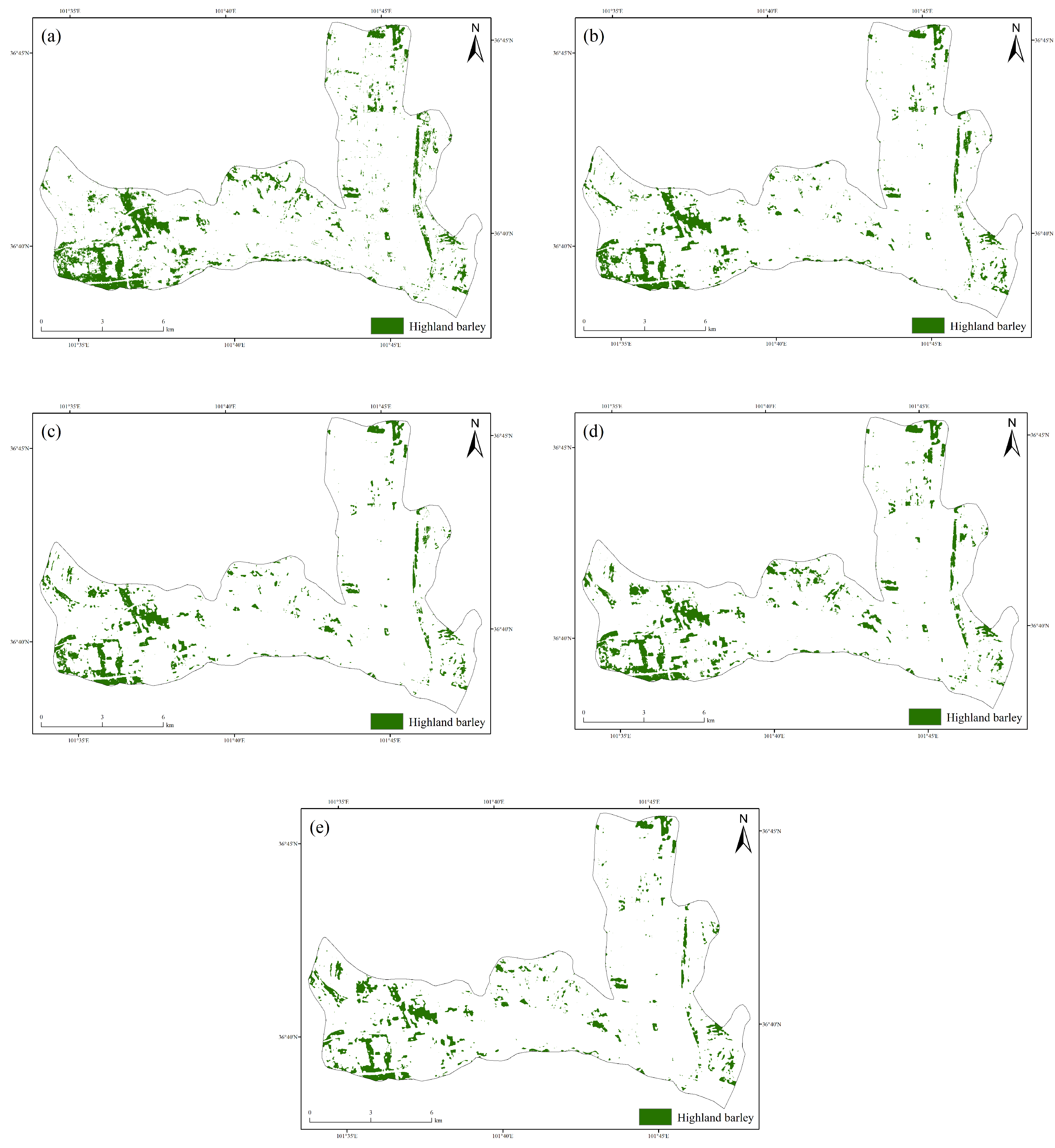
3.3. Analysis of Spatial Distribution of Highland Barley in Different Time Phases

QGIS was used on the feature preference combinations for classification prediction and classification model evaluation, in which the classification process was classified into the following categories: Highland barley, other crops, and mountainous areas. The results for urban areas and water bodies were extracted using ArcGIS 10.7 software. A thematic map was produced to show the spatial distribution of the results (Figure 5).

Figure 5 shows that the northern part of the city exhibited a more extensive distribution, with the majority of the crop concentrated in the western region. Conversely, less highland barley was concentrated in the mountainous areas, while more highland barley was distributed in the cultivated land near the mountainous areas. The distribution map shows that the northern part of the city had a more extensive highland barley distribution in June and July, while there was a reduced distribution in August. This was due to the highland barley in the northern part of the city maturing in late August, when some of the highland barley was harvested.

In order to more accurately quantify the information extraction for highland barley crops in different periods, the accuracy of the classification results was evaluated and UA and PA were selected. The specific calculation results are shown in

Table 6. Classification accuracy based on information extraction using Sentinel-2 feature selection combinations.

Phenophase	Jointing Stage		Heading Stage		Flowering Stage		Milk Ripening Stage		Maturity Stage
Evaluation Index	PA (%)	UA (%)	PA (%)	UA (%)	PA (%)	UA (%)	PA (%)	UA (%)	PA (%)	UA (%)
Highland Barley	89.65	88.53	90.24	82.51	91.86	82.80	95.87	86.39	93.85	87.51
Other Crops	48.36	77.18	30.77	50.16	37.68	45.61	40.77	45.21	30.14	67.46
Mountainous Areas	96.07	95.64	95.42	94.87	93.69	95.94	93.92	96.59	93.61	94.14
Urban Areas	99.09	84.47	95.70	91.95	98.79	91.06	98.48	91.17	99.61	79.31
Water Bodies	94.96	100.00	98.05	100.00	98.70	100.00	91.38	100.00	90.73	100.00
OA (%)	92.56		90.90		90.74		91.55		90.51
Kappa	0.86		0.82		0.82		0.84		0.82

. Based on the optimal combination of Sentinel-2 remote sensing image features, the four indexes of OA, kappa, PA, and UA were selected for information extraction. The overall classification accuracy was high. For highland barley crops, the overall accuracy at the jointing stage was 92.56%, with a kappa coefficient of 0.86. The overall accuracy at the heading stage was 90.90%, with a kappa coefficient of 0.82. The overall accuracy at the flowering stage was 90.74%, with a kappa coefficient of 0.82. The overall accuracy at the milk ripening stage was 91.55%, with a kappa coefficient of 0.84. The overall accuracy at the maturity stage was 90.51%, with a kappa coefficient of 0.82. From the producer accuracy and user accuracy values of the various land types, it could be seen that the information extraction and classification effects based on the feature optimization combinations were better and that the overall recognition effect of highland barley was good. The overall accuracy and kappa coefficients for mountainous areas, urban areas, and water bodies were also high. From a comparison of the classification accuracy for different land cover types, it could be seen that machine learning performed well at extracting Qingke, mountainous areas, urban areas, and water bodies. However, the overall performance and kappa coefficient for other crops were average, with poorer extraction results for other crops. This was due to the fact that different crops were classified into a single category and the presence of multiple crops affected machine recognition, leading to misclassification. Research indicated that the random forest algorithm performs well at identifying finely classified categories. It was also validated that the random forest algorithm achieves high extraction accuracy for Qingke and can be used for remote sensing crop recognition studies on Qingke.

4. Discussion

This study employed multitemporal Sentinel-2 imagery and the random forest algorithm for crop extraction and classification, leveraging the advantages of multitemporal imagery to identify the five general feature variables (GLCM_Mean, RVI, homogeneity, MAX, and GLCM_Correlation) that were essential for highland barley extraction. By utilizing Sentinel-2 images from different phenological stages of highland barley (jointing stage, heading stage, flowering stage, milk ripening stage, and maturity stage), features were constructed and selected for each phenological stage. The random forest classification algorithm demonstrated that the overall accuracy of the imagery from the different phenological stages exceeded 90%. Consequently, these five phenological stages were considered crucial for the extraction and classification of highland barley. These stages accurately captured the developmental characteristics of highland barley, providing reliable data support for growth monitoring, yield prediction, and quality assessment in agricultural production.

The data source selected for this study was Sentinel-2, due to the extensive research conducted by domestic and international scholars on crop classification using time-series remote sensing data. For example, the low spatial resolution of MODIS, the long revisit period of Landsat, and the limited number of spectral bands in GF1 WFV data all impact the accuracy and efficiency of crop classification to some extent. In contrast, Sentinel-2 data offer a 5-day revisit period and 10 m resolution multispectral data, which significantly enhance the accuracy and efficiency of crop classification, particularly due to the inclusion of three red edge bands that are sensitive to vegetation spectral characteristics [30].

Based on the high classification accuracy of the imagery data from the different phenological stages, five common feature variables were selected from the preferred features of each stage [31]. Therefore, subsequent highland barley extraction research should focus on these five feature variables to ensure high reliability.

In this study, multitemporal crop classification research was carried out. Compared to previous single-temporal research, the multitemporal image data could capture changes in crops throughout the growth period and provide richer information. They could also offer a deeper understanding of the growth status of highland barley at different phenological periods and could help us obtain the most suitable phenological period for the extraction of highland barley for subsequent research. Wang et al. [32] used two different classification methods to classify crops in single-temporal remote sensing images, but their classification results lacked reliability. Saini et al. [33] used single-temporal Sentinel-2 images to classify crops, but the classification accuracy of the RF and SVM methods was below 90%. This was mainly due to the fact that the single-phase images could not reflect the changes in the crops during the whole growth period, and the methods lacked the ability to identify some key growth period characteristics because, at some time points, the spectral characteristics of corn and wheat were similar and difficult to distinguish. In this study, the use of multitemporal data for crop classification could effectively improve the accuracy of classification because the data could capture changes in crops throughout the growth period and provide more abundant information. These changes included the growth cycle of crops, changes in spectral characteristics, etc., which were conducive to distinguishing different types of crops. At the same time, according to the image data from different phenological periods, five common feature variables for extracting highland barley were obtained, four of which were texture features while one was a vegetation index, indicating that texture features have good versatility for crop extraction and provide reference value for subsequent classification research.

In this study, a total of 33 feature variables were constructed, among which texture features and the red edge index particularly contributed to the classification. As shown in Figure 4, the red edge index NDVIre1 at the jointing stage had a higher importance score, reaching 0.1792, followed by several texture features. This was mainly because the red edge index utilizes the red edge region in the spectral reflectance characteristics of plants, that is, the transition region between red light and near-infrared light [34]. This region is highly sensitive to the chlorophyll content and physiological conditions of plants. Texture features can effectively distinguish between different species or varieties because the leaf and stem textures of different plants are specific [35]. These characteristics were particularly important when distinguishing highland barley from other crops.

5. Conclusion

In this study, 25 features, including spectral, red edge, vegetation, and texture features, were constructed based on Sentinel-2 satellite images. Using the recursive feature elimination algorithm and the RF algorithm, the optimal feature datasets of different phenological periods were determined and then the feature selection combination subsets of different phenological periods were used to identify and classify highland barley. The main conclusions were as follows:

(1)

The overall classification accuracy of information extraction was better after feature optimization and the combination of multitemporal image data. The optimal phenological periods for highland barley extraction were the jointing stage and the milk ripening stage. For highland barley crops, the overall accuracy at the jointing stage was 92.56%, with a kappa coefficient of 0.86. The overall accuracy at the milk ripening stage was 91.55%, with a kappa coefficient of 0.84.

(2)

The importance score of the red edge index based on the Sentinel-2 image data was higher in the feature selection combination. The red edge index had a higher contribution rate in the process of crop information extraction and classification.

(3)

The five characteristic variables—GLCM_Mean, RVI, homogeneity, MAX, and GLCM_Correlation—were applicable to the information extraction of crops in Chengbei District and played a very important role in the classification of different phenological periods. These five characteristic variables were stable and universal throughout the process of crop extraction.

In contrast to previous studies, this research introduced the impact of different phenological periods on highland barley extraction and identified the optimal phenological period and the most effective subset of feature variables for highland barley extraction. Therefore, future research on highland barley extraction should focus on the jointing stage of highland barley and pay particular attention to the five feature variables: GLCM_Mean, RVI, homogeneity, MAX, and GLCM_Correlation.

References

1. Wu, B.; Xiao, L. Research on Crop intelligent Image Recognition and Classification Based on Convolution Neural Network. J. Agric. Mech. Res. 2023, 45, 20–23, 29. [Google Scholar]
2. Yang, C.; Liu, H.H.; Zhang, C. UAV Hyperspectral Remote Sensing Image Crop Fine Classification Based on SVM and RF. Henan Sci. 2020, 38, 1987–1995. [Google Scholar]
3. Liang, H.H. Research on crop classification based on UAV hyperspectral remote sensing image. China S. Agric. Mach. 2022, 53, 38–41. [Google Scholar]
4. Zhang, R.H. Study on Field Crop Extraction based on UAV Visible Light Image and Random Forest Model. Hortic. Seed 2023, 43, 99–101. [Google Scholar]
5. Cheng, T.; Xing, X.C.; Chen, C. Sugarcane planting range extraction based on multi temporal remote sensing images. Sci. Surv. Mapp. 2023, 48, 137–143. [Google Scholar]
6. Bao, J.W.; Wu, L.T.Y.; Che, Y.W.; Liu, Z.H.; Liu, Z.X. Research on crop planting structure extraction methods based on GF-6 images. J. N. Agric. 2023, 51, 112–121. [Google Scholar]
7. Yan, J.Z.; Zhang, M.; Zhang, S.Y. Information Extraction of Main Crops in Eastern Qinghai Province Based on GEE Platform and MODIS NDVI Time Series. J. S. Univ. Nat. Sci. Ed. 2023, 45, 55–64. [Google Scholar]
8. Liu, J.W. Research on Extraction of Crop Spatial Planting Structure Based on Sentinel-2 Data. Geomat. Spat. Inf. Technol. 2022, 45, 62–64. [Google Scholar]
9. Xie, Y.; Wang, J.N.; Liu, Y. Research on Winter Wheat Planting Area Identification Method Based on Sentinel-1/2 Data Feature Optimization. Trans. Chin. Soc. Agric. Mach. 2024, 55, 231–241. [Google Scholar]
10. Shi, F.F.; Lei, C.M.; Xiao, J.S.; Li, F.; Shi, M.M. Classification of Crops in Complicated Topography Area Based on Multisource Remote Sensing Data. Geogr. Geo-Inf. Sci. 2018, 34, 49–55+2. [Google Scholar]
11. Faqe Ibrahim, G.R.; Azad, R.; Haidi, A. Improving Crop Classification Accuracy with Integrated Sentinel-1 and Sentinel-2 Data: A Case Study of Barley and Wheat. J. Geovis. Spat. Anal. 2023, 7, 22. [Google Scholar] [CrossRef]
12. Bao, J.W.; Yu, L.F.; Wulantuya; Xu, H.; Wuyundeji; Yu, W.Z. Research on crop remote sensing recognition method based on a random forest method—Take some areas of Arun Banner as an example. J. N. Agric. 2020, 48, 129–134. [Google Scholar]
13. Chen, J.; Li, H.; Liu, Y.F.; Chang, Z.; Han, W.J.; Liu, S.S. Crops identification based on Sentinel-2 data with multi-feature optimization. Remote Sens. Nat. Resour. 2023, 35, 292–300. [Google Scholar]
14. Zhang, L.; Gong, Z.N.; Wang, Q.W.; Jin, D.D.; Wang, X. Wetland mapping of Yellow River Delta wetlands based on multi-feature optimization of Sentinel-2 images. Natl. Remote Sens. Bull. 2019, 23, 313–326. [Google Scholar] [CrossRef]
15. Fabian, L.; Grégory, D. Defining the Spatial Resolution Requirements for Crop Identification Using Optical Remote Sensing. Remote Sens. 2014, 6, 9034–9063. [Google Scholar] [CrossRef]
16. José, M.; Peña, B.; Moffatt, K.N.; Richard, E.P.; Johan, S. Object-based crop identification using multiple vegetation indices, textural features and crop phenology. Remote Sens. Environ. 2011, 115, 1301–1316. [Google Scholar]
17. Zhang, M.; Wu, B.F.; Yu, M.Z.; Zou, W.T.; Zheng, Y. Crop Condition Assessment with Adjusted NDVI Using the Uncropped Arable Land Ratio. Remote Sens. 2014, 6, 5774–5794. [Google Scholar] [CrossRef]
18. Fernández-Manso, A.; Fernández-Manso, O.; Quintano, C. SENTINEL-2A red-edge spectral indices suitability for discriminating burn severity. Int. J. Appl. Earth Obs. Geoinf. 2016, 50, 170–175. [Google Scholar] [CrossRef]
19. He, Z.N.; Jing, M.; Han, H.T.; Liu, P.; Ji, F.; Chen, M.L. Sparse principal component analysis-random forest algorithm combined with optimized spectroscopy for identification of soil surface oil species. Chin. J. Anal. Lab. 2024, 3, 1–9. [Google Scholar]
20. Zhou, Z.H. Machine Learning: Development and Future. Commun. China Comput. Soc. 2017, 13, 44–51. [Google Scholar]
21. Li, X.D. Water quality assessment based on principal component analysis and water quality identification index: Taking Dongshan County of Fujian Province as an example. Jilin Geol. 2022, 41, 57–65. [Google Scholar]
22. Haralick, R.M. Statistical and structural approaches to texture. Proc. IEEE 1979, 67, 786–804. [Google Scholar] [CrossRef]
23. Wang, L.X.; Shi, Z.T.; Xi, W.F.; Li, G.Z.; Yang, Z.R. Research on Extraction of Bedrock Landslide Texture Feature Based on Gray Co-occurrence Matrix. Urban Geotech. Investig. Surv. 2023, 2, 187–192. [Google Scholar]
24. Iverson, L.R.; Prasad, A.M.; Matthews, S.N.; Peters, M. Estimating potential habitat for 134 eastern US tree species under six climate scenarios. For. Ecol. Manag. 2008, 254, 390–406. [Google Scholar] [CrossRef]
25. Breiman, L. Random forest. Mach. Learn. 2001, 45, 5–32. [Google Scholar] [CrossRef]
26. Ou, D.J. Hyperspectral Remote Sensing Image Classification Based on Multi-Classifier Fusion. Master’s Thesis, Shandong University, Jinan, China, 2019. [Google Scholar]
27. Sun, R.X.; Shen, M.S.; Hu, Y.W.; Xu, Q.T.; Zhang, J.J. Effect of Grass Belt Distribution on Runoff and Sediment Yield Under Simulated Rainfall. J. Soil Water Conserv. 2022, 36, 22–29. [Google Scholar]
28. Yang, Y.G.; Liu, P.; Zhang, H.B.; Zhang, W.Z. Research on GF-2 Image Classification Based on Feature Optimization Random Forest Algorithm. Spacecr. Recovery Remote Sens. 2022, 43, 115–126. [Google Scholar]
29. Tao, L.; Hu, Z.L. Crop planting structure identification based on Sentinel-2A data in hilly region of middle and lower reaches of Yangtze River. Bull. Surv. Mapp. 2021, 7, 39–43. [Google Scholar] [CrossRef]
30. Huang, Q.Y.; Li, L.; Xue, P.; Ying, G.W. Main Crop Classification Based on Multi-temporal Sentinel-2 Data in Chengdu Plain. Geomat. Spat. Inf. Technol. 2024, 47, 65–68. [Google Scholar]
31. Rashmi, S.; Kumar, S.G. Crop classification in a heterogeneous agricultural environment using ensemble classifiers and single-date Sentinel-2A imagery. Geocarto Int. 2019, 36, 2141–2159. [Google Scholar]
32. Wang, L.J.; Guo, Y.; He, J.; Wang, L.M.; Zhang, X.W.; Liu, T. Classification Method by Fusion of Decision Tree and SVM Based on Sentinel-2A Image. Trans. Chin. Soc. Agric. Mach. 2018, 49, 146–153. [Google Scholar]
33. Saini, R.; Ghosh, K.S. Crop classification on single date Sentinel-2 imagery using random forest and suppor vector machine. ISPRS-Int. Arch. Photogramm. Remote Sens. Spat. Inf. Sci. 2018, 42, 683–688. [Google Scholar] [CrossRef]
34. Jiang, Y.R.; Ye, J.; Xie, Z.L.; Li, X.H. Rape planting extraction based on phenological characteristics analysis of time series Sentinel-2 images. J. Chengdu Univ. Technol. Sci. Technol. Ed. 2024, 4, 15–28. [Google Scholar]
35. Song, Y.B.; Xiao, C.; Zhao, Y.F.; Wang, Y.C. Research on crop remote sensing classification method based on growth spatio-temporal information. China S. Agric. Mach. 2023, 54, 49–51. [Google Scholar]
Figure 1. Geographical location and sample points of the research area.
Agriculture 14 01466 g001
Figure 2. Flow chart of crop information extraction process.
Agriculture 14 01466 g002
Figure 3. Relationship between the number of feature variables and classification accuracy in terms of maturity stage.
Agriculture 14 01466 g003
Figure 4. Importance ranking of characteristic variables in terms of the jointing stage.
Agriculture 14 01466 g004
Figure 5. Spatial distribution of highland barley in the study area during different phenological periods: (a) jointing stage, (b) heading stage, (c) flowering stage, (d) milk ripening stage, (e) maturity stage.
Agriculture 14 01466 g005