Abstract
Timely and accurate mapping of rice distribution is crucial to estimate yield, optimize agriculture spatial patterns, and ensure global food security. Feature selection (FS) methods have significantly improved computational efficiency by reducing redundancy in spectral and temporal feature sets, playing a vital role in identifying and mapping paddy rice. However, the optimal feature sets selected by existing methods suffer from issues such as information redundancy or local optimality, limiting their accuracy in rice identification. Moreover, the effects of these FS methods on rice recognition in various machine learning classifiers and regions with different climatic conditions and planting structures is still unclear. To overcome these limitations, we conducted a comprehensive evaluation of the potential applications of major FS methods, including the wrapper method, embedded method, and filter method for rice mapping. A novel hierarchical lustering sequential forward selection (HCSFS) method for precisely extracting the optimal feature set for rice identification is proposed. The accuracy of the HCSFS and other FS methods for rice identification was tested with nine common machine learning classifiers. The results indicated that, among the three FS methods, the wrapper method achieved the best rice mapping performance, followed by the embedded method, and lastly, the filter method. The new HCSFS significantly reduced redundant features compared with eleven typical FS methods, demonstrating higher precision and stability, with user accuracy and producer accuracy exceeding 0.9548 and 0.9487, respectively. Additionally, the spatial distribution of rice maps generated using the optimal feature set selected by HCSFS closely aligned with actual planting patterns, markedly outperforming existing rice products. This research confirms the effectiveness and transferability of the HCSFS method for rice mapping across different climates and cultivation structures, suggesting its enormous potential for classifying other crops using time-series remote sensing images.
1. Introduction
Rice is one of the most important staple foods globally, feeding more than half of the world’s population [1,2]. In addition, rice cultivation necessitates precise management of water resources. Thus, timely and accurate monitoring of rice cultivation is essential for yield forecasting, optimizing agriculture spatial patterns, allocating resources effectively, and fostering sustainable agricultural development [3,4]. The availability of numerous freely accessible remote sensing images, such as those from Landsat and Sentinel, has facilitated the rapid production of large-scale crop classification maps through remote sensing technology [5,6].
Remote sensing imagery provides extensive spectral information for rice mapping, effectively distinguishing the spectral features of rice from those of other crops. Various spectral features are employed to monitor the moisture content, pigment deposition, and coverage of rice [7,8,9]. However, dependence on a limited number of spectral bands or vegetation indices may not produce accurate maps, especially in areas with complex cropping structures [10,11]. Rice exhibits flooding signals during the transplanting phase and thrives during the growth phase and displays signs of aging and yellowing during the maturity phase that are significantly different from those of other crops. Consequently, multi-temporal images can capture spectral features of rice across various phenological stages, offering significant advantages over single-temporal images [12,13,14]. Increasingly, researchers are able to identify crop types by extracting phenological information from time-series images. For example, spectral and temporal features from Sentinel-2 were input into a deep learning model to map the main crops across six counties in the United States [15]. Multi-temporal Landsat imagery, combined with phenology-based machine learning models, generated rice maps for Heilongjiang Province, China, from 1990 to 2020 [16]. Time-series harmonized Landsat and Sentinel-2 (HLS) data were utilized to produce accurate rice maps [17]. These studies generally classified crops using spectral and temporal features extracted from all available images [18]. However, this straightforward superposition of time-series images substantially elevates the number of features, potentially resulting in numerous redundant features and increased computation time [19,20]. Additionally, it may obscure critical phenological information, thereby diminishing the accuracy and generalizability of rice identification methods [21]. Therefore, selecting appropriate spectral and temporal features from vast satellite datasets to accurately identify rice poses a significant challenge.
Numerous studies have investigated the use of feature selection (FS) methods to identify optimal spectral and temporal feature sets for crop mapping [21,22]. FS methods can be categorized into embedded methods (e.g., random forest [23]), filter methods (e.g., JM distance [24]), and wrapper methods (e.g., recursive feature elimination [25]). Among these methods, the embedded method ranks features importance based on specific algorithms. For example, Zhu et al. employed the random forest (RF) model to assess feature importance across all dates, selecting 28 features with importance greater than 0.8 for tea garden identification [26]. However, this approach neglects feature collinearity, and the optimal feature set obtained usually includes numerous redundant features, necessitating further filtering [27]. Additionally, filter methods leverage the relationships among features to evaluate their importance. Hu et al. proposed a phenology-based method for choosing 34 spectral–temporal features for mapping corn in Heilongjiang Province, China [21]. While the filter method enhances feature selection efficiency and balances the separability among features, it tends to retain a substantial number of features and does not consider the impact of the individual feature on classification performance. As a result, the feature subsets generated may not be optimal for the target [28]. In contrast, the wrapper method combines prediction results of machine learning algorithms to assess each feature’s impact on classification performance, selecting the features with the highest contribution as the optimal feature set. Shafiee et al. combined sequential forward selection (SFS) with support vector regression (SVR) to select the optimal spectral features and accurately predict the yield of 600 spring wheat plots in southeastern Norway [29]. However, when comparing SFS with LASSO, they found that SFS still exhibited lower accuracy, the reason being that commonly used wrapper methods such as SFS [30], sequential backward selection (SBS) [31], and RFE are greedy algorithms that focus solely on accuracy, often converging to local optima and potentially overlooking valuable features that could improve classification results [32]. These challenges make it hard to determine the optimal spectral and temporal feature sets for producing high-quality spatial distribution maps of rice. Furthermore, the impact of these FS methods on rice recognition across different machine learning algorithms and regions with diverse planting structures and climatic conditions remains unclear.
To address the above issues, we systematically evaluated the application of principal FS methods in rice mapping. We propose a novel hierarchical clustering sequential forward selection (HCSFS) method. The HCSFS utilizes the hierarchical clustering (HC) algorithm to group features, followed by the SFS method to eliminate features with lower contributions within each group. These FS methods were tested in Sichuan and Jiangsu provinces, China, which exhibit significant differences in climate and crop-planting structures. Since machine learning classifiers have been widely applied for large-scale crop mapping [22], we inputted the optimal feature sets, selected from the original data by the HCSFS method and 11 other FS methods, into nine commonly used machine learning algorithms to identify rice. The accuracy of each FS method was validated with ground samples, to assess the stability of their integration with different machine learning models.
The contributions of this article are as follows:
- (1)
- The potential of key FS methods in rice mapping is comprehensively evaluated;
- (2)
- A robust HCSFS method is proposed to address the issues of feature redundancy and local optimization in existing FS methods;
- (3)
- The new method demonstrates effective transferability across different spatial contexts (regions with different agricultural planting structures and climates) and temporal contexts (early identification), thereby offering advanced technical support for precision agriculture.
2. Materials and Methods
2.1. Study Area
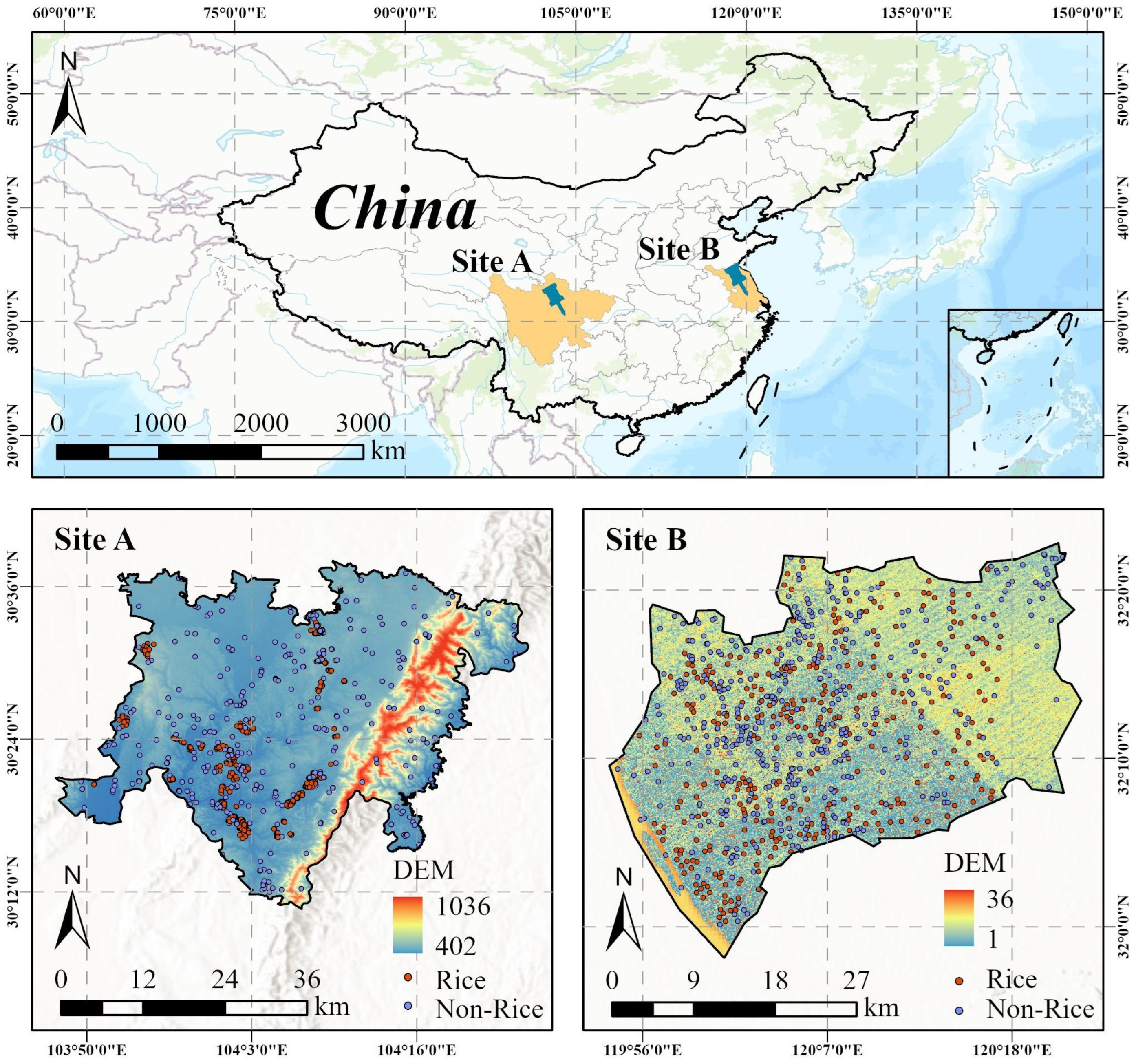
Two sites with distinct climatic conditions and crop planting structures were selected as the research areas (Figure 1). Site A is located in the Tianfu New Area, Sichuan Province (103°48′–104°25′ E, 30°11′–30°38′ N), within the Chengdu Plain. It spans 1578 square kilometers, with elevations ranging from 402 to 1036 m. The terrain varies considerably, with the north predominantly flat, the east mountainous, and the remaining areas hilly. Site A experiences a subtropical monsoon climate, with an average annual precipitation of approximately 855.8 mm and an average temperature of 16.3 °C. The planting structure of the location is complex, including rice, corn, soybeans, vegetables, loquat, strawberries, citrus, and so on. Site B, situated in Taixing City, Jiangsu Province (119°54′–120°22′ E, 31°58′–32°23′ N), within the alluvial plain of the Yangtze River Delta, covers 1172.27 square kilometers with a gentle slope. The climate is characterized by an average annual precipitation of 1031.8 mm and an average temperature of 14.90 °C. At site B, rice cultivation is predominant during the summer season. Figure 2 provides the crop calendars for both study areas.

Figure 1.
Study area and sample points.
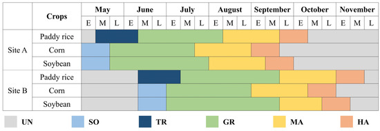
Figure 2.
The calendar of main crops at each study site. Abbreviations for various periods: unplanted period (UN), sowing period (SO), transplanting period (TR), growing period (GR), maturity period (MA), harvest period (HA).
2.2. Data
2.2.1. Sentinel-2 Imagery
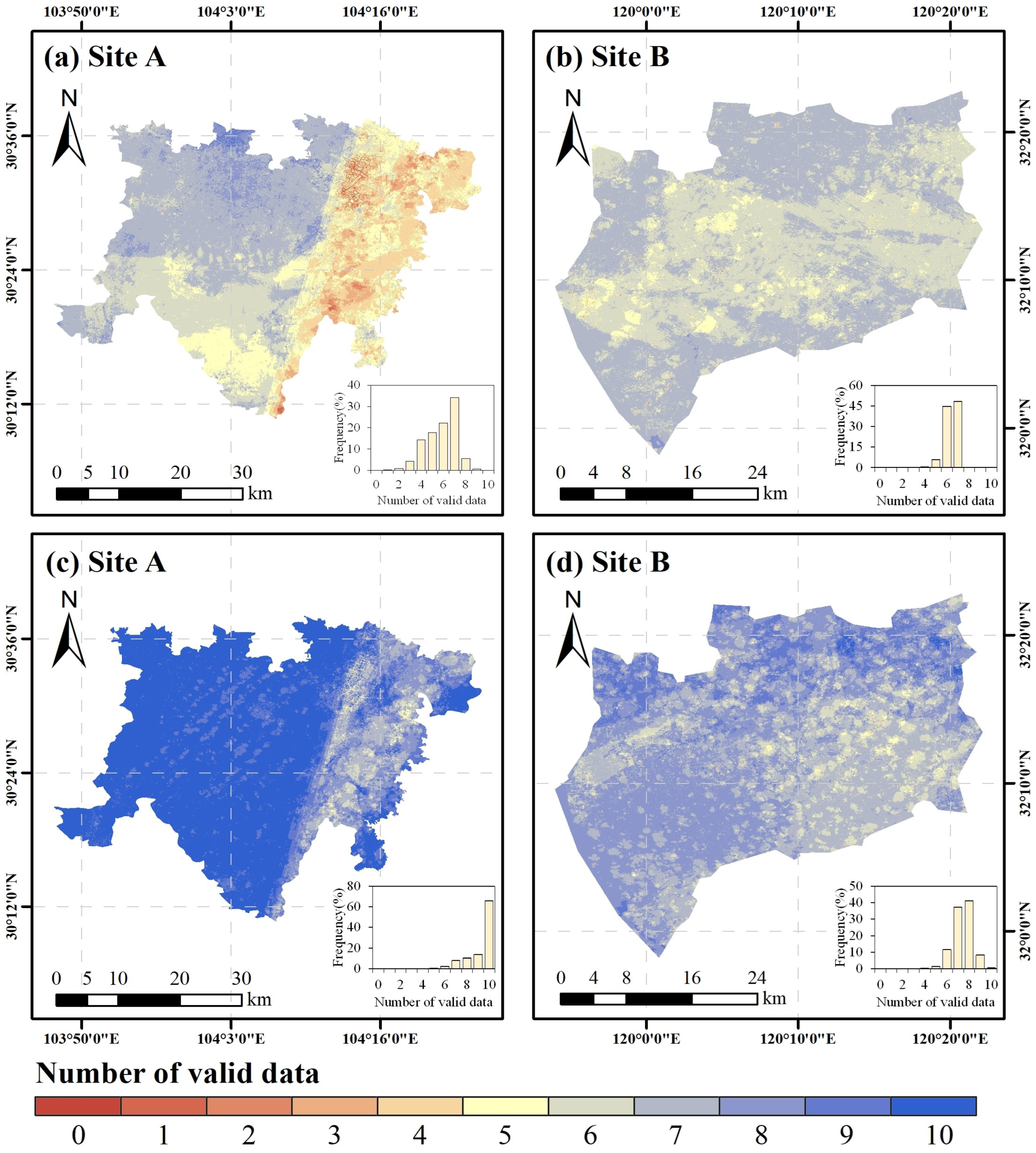
This study quantified the frequency of effective Sentinel-2 observations at two sites during their respective rice-growing seasons (Site A: May 16 to October 12, Site B: June 16 to November 13) using 1-year and 3-year 15-day intervals, respectively (Figure 3). Based on one year of Sentinel-2 observation data at site A, 5.52% of observations were recorded 0–3 times, predominantly in the eastern mountainous area. Additionally, 54.15% of observations occurred 4–6 times and 40.33% occurred 7 times or more across the entire site (Figure 3a). Meanwhile, at site B, observations recorded 4–6 times accounted for 51.13% in most areas, with only 0.3% occurring 8 times or more (Figure 3b). These findings highlight the challenges of relying solely on one year of Sentinel-2 imagery to obtain comprehensive phenological data for rice. To address this challenge, Ni et al. synthesized Sentinel-2 imagery from the target year and adjacent years, successfully creating high-quality rice maps of northeast China [33]. The analysis of three-year composite imagery in this study revealed that the majority of observations at both site A and site B predominantly occurred 7 to 10 times, accounting for 97.34% and 87.08%, respectively (Figure 3c,d). This emphasizes the value of using triennial composites to reduce cloud-cover interference. Therefore, we selected all valid Sentinel-2A images covering the two sites in the Google Earth Engine (GEE) during the three-year rice growing season as the input data.
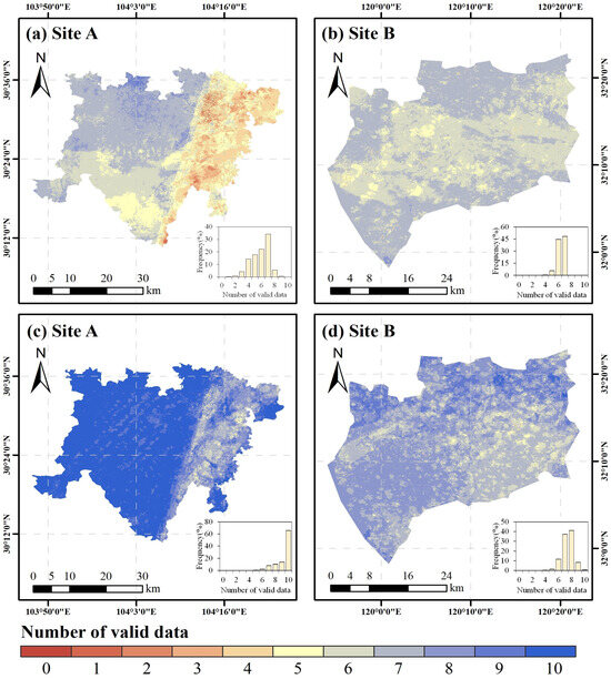
Figure 3.
Numbers of valid data during the rice growth period at sites A and B in one year ((a): 2022, (b): 2020) and three years ((c): 2021–2023, (d): 2019–2021).
2.2.2. Validation Data
Ground truth data for rice were collected at site A in June 2022 and site B in July 2020, respectively (Figure 1). The coordinate and crop type for each sample (e.g., rice, corn, soybean, and others) were recorded using a handheld GPS device. Additionally, non-cultivated land samples (e.g., garden, forest, grass, water, building, and bare soil) were identified by manual interpretation of high-resolution images from Google Earth. All sample points were randomly split into two groups in an approximately 1:1 ratio for training and validation purposes. Table 1 shows the number of samples selected at the two sites. Additionally, we acquired rice product data (Shen-TWDTW) from Shen et al. to validate the spatial details of the rice map [34].

Table 1.
Sample number information for the two study sites.
2.3. Overview of Methods
A novel feature selection method, HCSFS, is proposed in this paper. This method was integrated with a machine learning algorithm to accurately identify rice at two research sites (Figure 4). The overall workflow included (1) constructing time-series spectral feature sets on the GEE, (2) evaluating the performance of the optimal feature sets selected by the HCSFS and common FS methods for rice identification, and (3) quantitatively assessing the rice mapping results using ground truth samples and comparing them with advanced FS methods and existing mapping products.
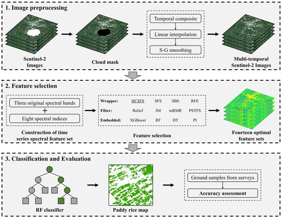
Figure 4.
Overall workflow of this study.
2.4. Construction of Time-Series Spectral Feature Sets
This study processed Sentinel-2 original images through four steps to obtain cloud-free and complete time-series data. The steps were as follows: (1) Removing clouding from the Sentinel-2 original data using the Sentinel-2 cloud probability map in the GEE; (2) Generating Sentinel-2 time series data through 15-day median synthesis; (3) Filling in missing pixels using linear interpolation to ensure coverage of the entire time-series images [35]; (4) Applying the Savitzky–Golay (SG) filter to smooth the time-series data [36]. Specifically, a third-order SG filter with a window size of 135 days (9 observations) was used for this study.
This study employed common feature sets for identifying rice, consisting of three original spectral bands and eight spectral indices (Table 2). The three spectral bands included Red Edge2 (RE2), shortwave infrared band1 (SWIR1), and shortwave infrared band2 (SWIR2). The eight spectral indices comprised the Normalized Difference Vegetation Index (NDVI), Enhanced Vegetation Index (EVI), Land Surface Water Index (LSWI), Normalized Difference Senescent Vegetation Index (NDSVI), Normalized Difference Tillage Index (NDTI), Red Edge NDVI (RENDVI), Red Edge Position (REP), and Plant Senescence Reflection Index (PSRI).
Table 2.
Details of the spectral indices.
2.5. Feature Selection
2.5.1. HCSFS
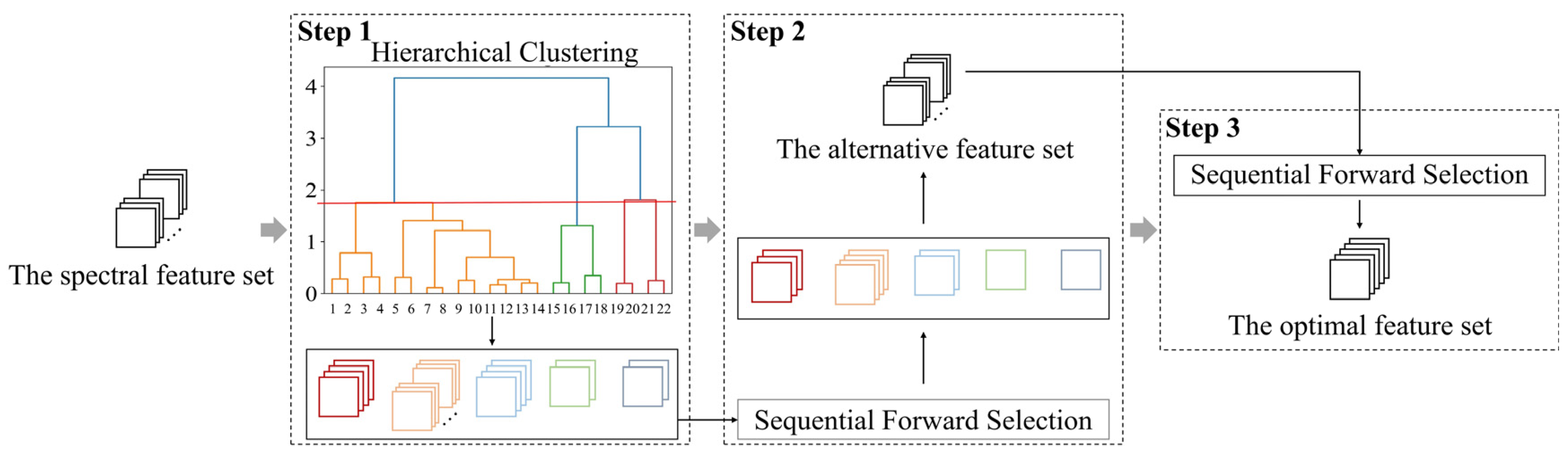
The SFS method has been widely adopted for feature selection owing to its high accuracy and straightforward principles. In this paper, we extend SFS by integrating the HC algorithm, introducing a novel approach called HCSFS. The workflow for selecting optimal spectral features is shown in Figure 5.

Figure 5.
The workflow of HCSFS.
Firstly, the HC was used to categorize the time-series spectral feature set into distinct classes. For a more intuitive depiction of feature relationships, Spearman rank correlation was employed instead of the traditional Euclidean distance [27]. The formula for calculating the Spearman rank correlation between two features is as follows:
where ρ refers to the Spearman rank correlation of two features x and y, xi and yi represent the i-th sample in x and y, and represent the rank of xi and yi, and and represent the average rank of x and y, respectively. If there are multiple samples with the same value, their ranks are averaged. The range of ρ is from −1 to 1, and a larger absolute value of ρ indicates a higher correlation between x and y. The value of n represents the number of samples.
The average-linkage clustering method was employed to hierarchically cluster all features in the Spearman rank correlation matrix. The clustering process involved the following steps [39]: (1) each feature was initially assigned to a separate category; (2) the two features exhibiting the highest correlation among all features were merged into one category; (3) the new category was recalculated with the average distance among other classes; (4) Steps 2 and 3 were repeated until all categories were merged into a single class; (5) Finally, the appropriate number of clusters was determined by a distance threshold. The average distance was calculated as follows:
where C1 and C2 are two feature classes, dij represents the distance between the feature i in C1 and the feature j in C2, and n1 and n2 represent the number of features in C1 and C2, respectively. The initial distance between two features is equal to the Spearman rank correlation between them.
Secondly, SFS was used to filter features within each category and aggregate the selected features into an alternative feature set. The SFS process began with an empty feature subset. Each feature from the time-series spectral feature set was individually added to the subset, which was subsequently fed into the machine learning classifier to assess the overall accuracy (OA) of the newly formed subset. The feature that most improved the subset’s OA was retained in the subset and removed from the spectral feature set. This procedure was iteratively repeated until adding new features no longer enhanced the subset’s OA [30].
Thirdly, the SFS was employed again to refine the alternative feature set and obtain the optimal feature set to identify paddy rice. The HCSFS method addresses the limitations of wrapper methods, which often overlook feature correlations, thereby ensuring that feature selection avoids local optima.
2.5.2. Other Feature Selection Methods
To systematically evaluate the application of three types of FS methods in rice mapping, we selected four representative methods from each category. In the wrapper methods, we selected original SFS [40], SBS [31], and RFE [22] to compare with HCSFS. HCSFS and SFS are forward selection methods, whereas SBS and RFE are categorized as backward selection methods. Additionally, we selected JM distance [41], Relief [42], Max-Relevance and Min-Redundancy (mRMR) [43], and phenology-based spectral and temporal feature selection (PSTFS) [21] as representatives of the filter methods. Notably, PSTFS has been extensively utilized in crop identification [17,21,44]. In this study, to ensure consistency in the criteria for eliminating redundant features, we calculated Pearson correlation coefficients for each pair of features within the spectral feature set, to evaluate the need to eliminate highly correlated features in filter methods [21]. Lastly, for embedded methods, we selected XGBoost [45], RF [27], decision tree (DT) [46], and ranking importance (PI) [47]. For the embedded methods, after ranking features by importance from highest to lowest, the top n features with the highest OA were chosen as the optimal feature set. All FS methods were executed in a local Python environment. The RFE, DT, RF, and PI methods were implemented using the ‘sklearn’ module, while the Relief, mRMR, and XGBoost methods were executed via the ‘skrebate’, ‘mrmr’, and ‘xgboost’ modules, respectively. Custom scripts were employed for other FS methods, such as HCSFS, SFS, and JM. Default parameters were set for all methods, and a random state of 42 was consistently applied to ensure uniformity across all runs.
2.6. Classification and Evaluation
This study evaluated the performance of the HCSFS along with 11 FS methods, using nine machine learning models including RF, gradient-boosting decision tree (GBDT), ExtraTrees (ET), AdaBoost, XGBoost, DT, naive Bayes (NB), K-nearest neighbor (KNN), and support vector machine (SVM). These algorithms have been widely applied to crop classification studies [22,48,49,50,51,52,53]. All classifiers were executed within the same local Python environment, with the RF, GBDT, ET, AdaBoost, DT, NB, KNN, and SVM classifiers sourced from the ‘sklearn’ module, while the XGBoost classifier was derived from the ‘xgboost’ module. All classifiers were operated with the modules’ default parameters, and the random state was also consistently set to 42.
In addition, three assessment indicators were determined by establishing a confusion matrix, including OA, user accuracy (UA), producer accuracy (PA), and F1 score, to evaluate the mapping accuracy of FS methods such as HCSFS for each classifier [54,55]. The verification indicators were calculated using the following equations (Equations (3)–(6)):
where ntp (true positive) represents the number of pixels that correctly classify rice as rice, while ntn (true negative) represents the number of pixels that correctly classify non-rice as non-rice. nfp (false positive) refers to the number of pixels that correctly classify non-rice as rice, and nfn (false negative) refers to the number of pixels that correctly classify rice as non-rice.
Finally, this study integrated the three best FS methods—HCSFS, SFS, and PSTFS— with the RF classifier to generate three paddy mapping frameworks: HCSFS-RF, SFS-RF, and PSTFS-RF. The generated rice maps were compared in spatial detail and against Shen-TWDTW.
3. Results
3.1. Comparison of HCSFS with Other Methods
3.1.1. The Number of the Optimal Feature Sets
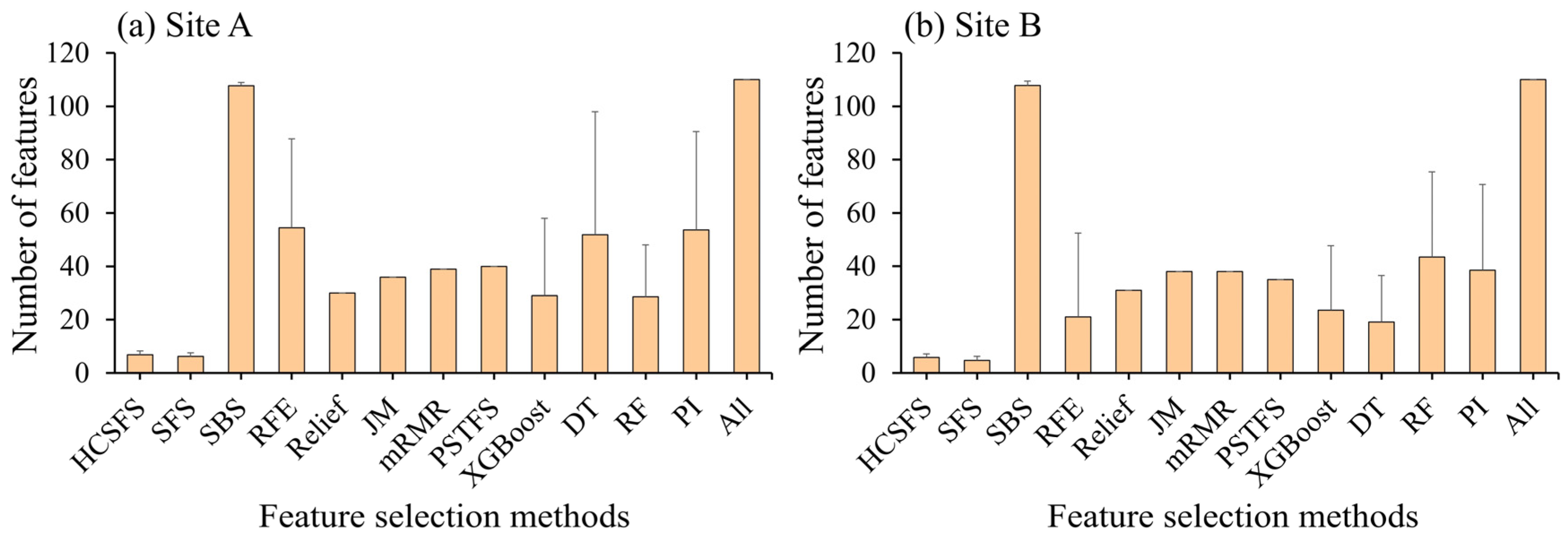
Figure 6 presents the number of optimal feature sets obtained by twelve different FS methods across two study areas. These data stem from nine trials employing nine classifiers, with the final column denoting the total count of original spectral feature sets. Compared with the backward selection methods (SBS and RFE), the forward selection methods (HCSFS and SFS) exhibited significantly smaller numbers and standard deviation in the selected optimal feature set. This highlights the stability of the forward selection methods for eliminating redundant features. However, the number of optimal feature sets obtained by the four filter methods (Relief, JM, mRMR, and PSTFS) did not vary, indicating that they were independent of the classifier. Despite removing a large number of highly correlated features through the Pearson correlation coefficient, the number of feature combinations generated by these methods remained significantly higher than that of the HCSFS and SFS. Lastly, the number and standard deviation of the optimal feature combinations selected by the four embedded methods (XGBoost, DT, RF, and PI) were relatively large, indicating that employing feature importance ranking introduced higher uncertainty in the feature count determination. Thus, our proposed HCSFS method effectively eliminated a substantial number of redundant features, thereby markedly reducing the training workload of the machine learning models and enhancing the efficiency of rice mapping.

Figure 6.
Average number of optimal feature sets obtained by combination of different feature selection methods and 9 classifiers.
3.1.2. Accuracy Stability of Feature Selection Method
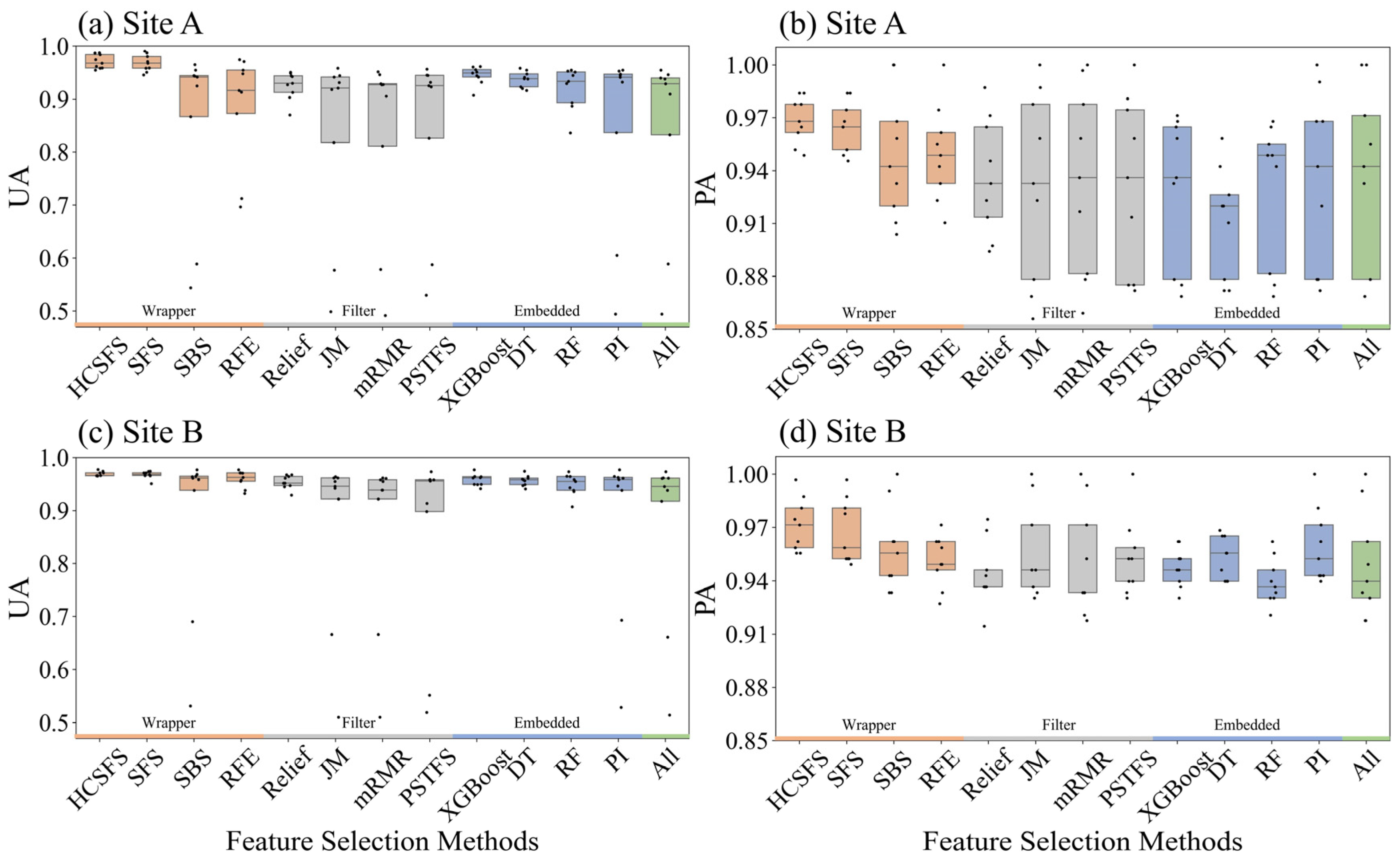
The study evaluated rice identification performance by employing a combination of 12 FS methods and 9 typical machine learning models (Figure 7). The results indicate that most FS methods exhibited smaller deviations in accuracy at site B compared with site A. This suggests that rice identification with higher accuracy stability can be achieved in regions with simple topography and planting structures. Importantly, the extent to which these methods improved the accuracy of rice identification varied: wrapper methods generally achieved higher accuracy than embedded methods, and embedded methods generally outperformed filter methods. This implies that combining feature selection with classifiers enhances the effectiveness of selecting features that accurately identify rice. Among the filter methods, the PSTFS exhibited a notably higher median. Additionally, compared with the other filter methods, the Relief showed the smallest fluctuations in UA and PA, maintaining values above 0.85 across all classifiers. Among the embedded methods, the XGBoost demonstrated a more compact range in its boxplot compared with the other three methods, with its median UA close to the upper quartile of the DT, RF, and PI. Among the wrapper methods, there was a noticeable difference in the precision range among the four methods, with the two forward selection methods (HCSFS and SFS) clearly outperforming the two backward selection methods (SBS and RFE). Particularly, the HCSFS achieved the highest precision stability, with median UA and PA exceeding 0.96. Overall, the SFS demonstrated the highest accuracy among the existing traditional FS methods, whereas mRMR exhibited the poorest performance in rice identification. HCSFS further enhanced rice identification accuracy, particularly with high PA, indicating reduced missed recognitions while maintaining a compact feature set (Figure 6).
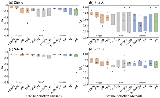
Figure 7.
The box plots of rice UA (a,c) and PA (b,d) obtained by combination of different feature selection methods and 9 classifiers at sites A and B. (“All” means using all the 110 features).
3.2. Separability of the Optimal Feature Sets
Table 3 presents the optimal feature sets selected by the advanced HCSFS and SFS methods, utilizing an RF classifier, at sites A and B. Both methods included common features as well as distinguishing features in the feature sets selected at the two sites. To compare the effectiveness of the feature sets selected by the HCSFS and SFS in distinguishing between rice and non-rice samples, t-SNE scatter plots for each feature set were generated (Figure 8). In Figure 8a,c, corresponding to the HCSFS, rice and non-rice samples demonstrate distinct left-right and top-bottom distributions within the two-dimensional space. The rice samples are tightly clustered, exhibiting a high degree of internal consistency. Concurrently, the non-rice samples also show a tendency to cluster in distinct directions, with an apparent demarcation from the rice samples. This differentiation can be attributed to the diversity of non-rice samples, such as corn, soybeans, forests, and so on. In contrast, Figure 8b,d show rice and non-rice samples that cross and overlap each other in the feature space without significant boundaries or clustering trends. These findings highlight the need for optimization of the SFS and demonstrate the effectiveness of the HCSFS in extracting the optimal feature set for rice identification.
Table 3.
The optimal feature sets selected by the HCSFS and SFS at two sites.
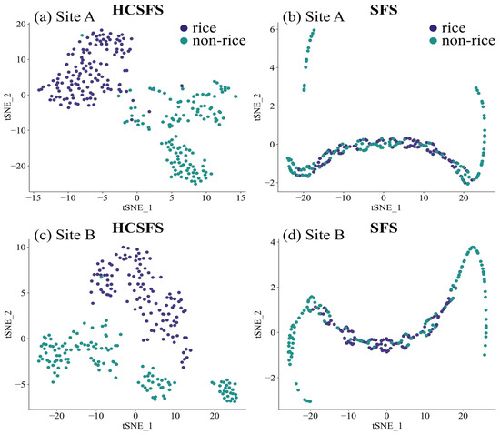
Figure 8.
tSNE visualizations obtained from the optimal feature sets selected by HCSFS and SFS at sites A (a,b) and B (c,d).
3.3. Quality Assessment of Paddy Rice Maps
3.3.1. Paddy Rice Probability Maps—HCSFS
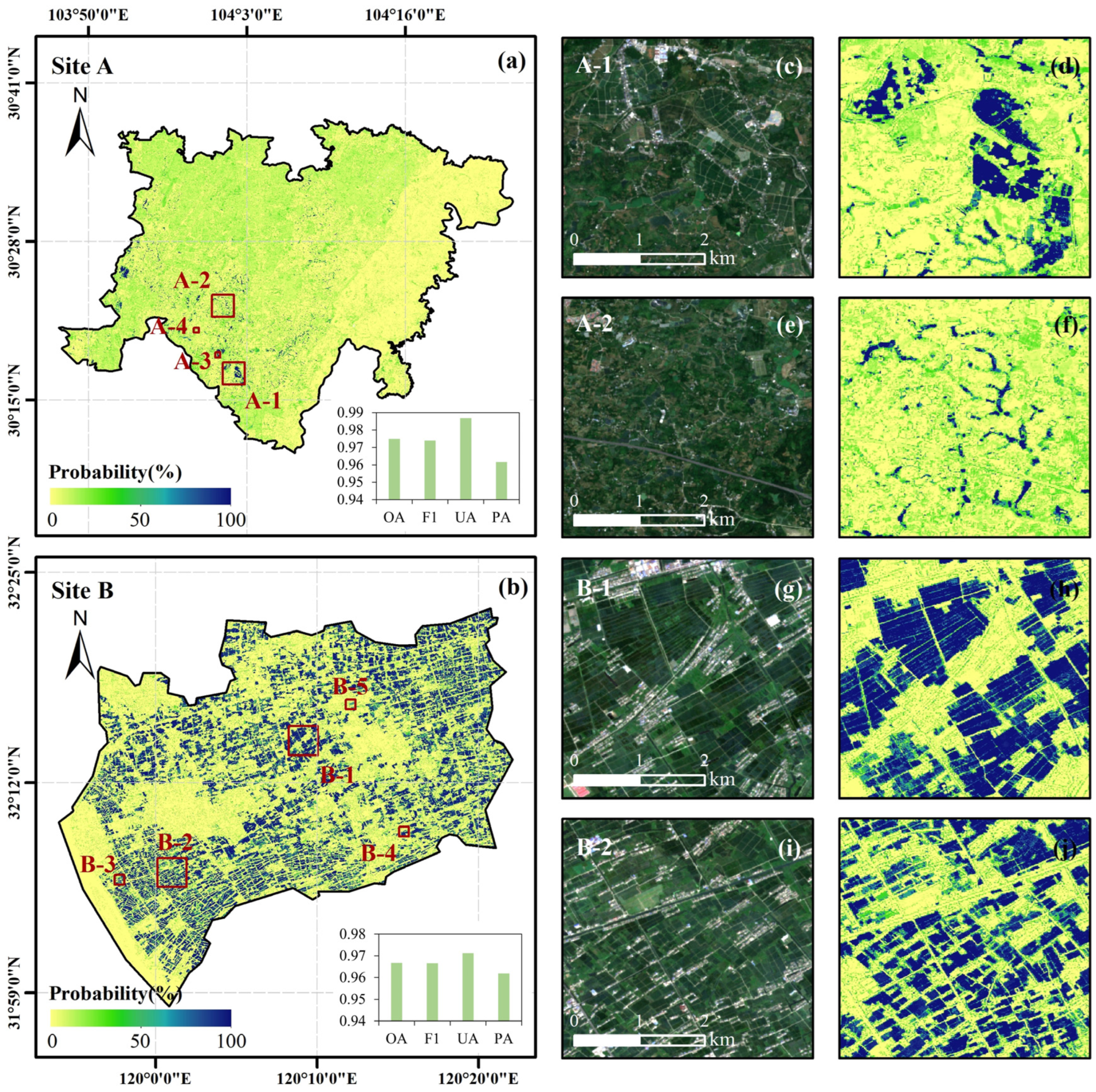
To illustrate the spatial distribution of rice cultivation and associated classification uncertainty, this study used the HCSFS-RF framework to generate 10 m spatial resolution rice probability maps for sites A and B (Figure 9). Figure 9a,b comprehensively shows the scale and probability distribution of paddy rice at both sites, while Figure 9c–j offers zoomed-in views of the detailed areas marked by red rectangles A-1, A-2, B-1, and B-2 in Figure 9a,b. Despite minor salt and pepper noise in the rice paddy maps, a comparison with Sentinel-2 true-color imagery confirmed that the spatial probability distribution of paddy rice aligned with actual cultivation patterns. In Sichuan Province, site A features smaller fields with scattered rice cultivation, predominantly located in the flat valleys of the southwestern region (Figure 9a). The eastern region is distinguished by the north–south orientation of the Longquan Mountains. With high altitudes and complex terrain, the likelihood of rice cultivation is exceedingly low. Figure 9d,f demonstrate the optimal feature set selected by HCSFS, effectively distinguishing paddy rice from ponds. At site B, in Jiangsu Province, characterized by large-scale cropland and intensive rice cultivation, paddy rice dominates much of the area. The enlarged mapping results (Figure 9h,j) accurately classify narrow roads and rivers within dense plots. Additionally, pixels with a recognition probability exceeding 50% were defined as rice, and 640 and 630 samples from the two study areas were used to evaluate the accuracy of the rice maps at sites A and B, respectively. The OA and F1-score of the rice maps obtained based on the HCSFS-RF framework were 0.9750 and 0.9740 at site A, and 0.9667 and 0.9665 at site B.
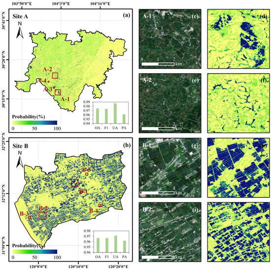
Figure 9.
Spatial probability distribution map of paddy rice and four enlarged views with paddy rice. (a,b) are the spatial probability distribution maps of rice at two sites. (c,e,g,i) show enlarged views with true-color composited Sentinel-2 images in the heading period. (d,f,h,j) show enlarged views with spatial probability distribution maps of rice.
3.3.2. Comparison of Rice Spatial Distribution Map of in Different Methods
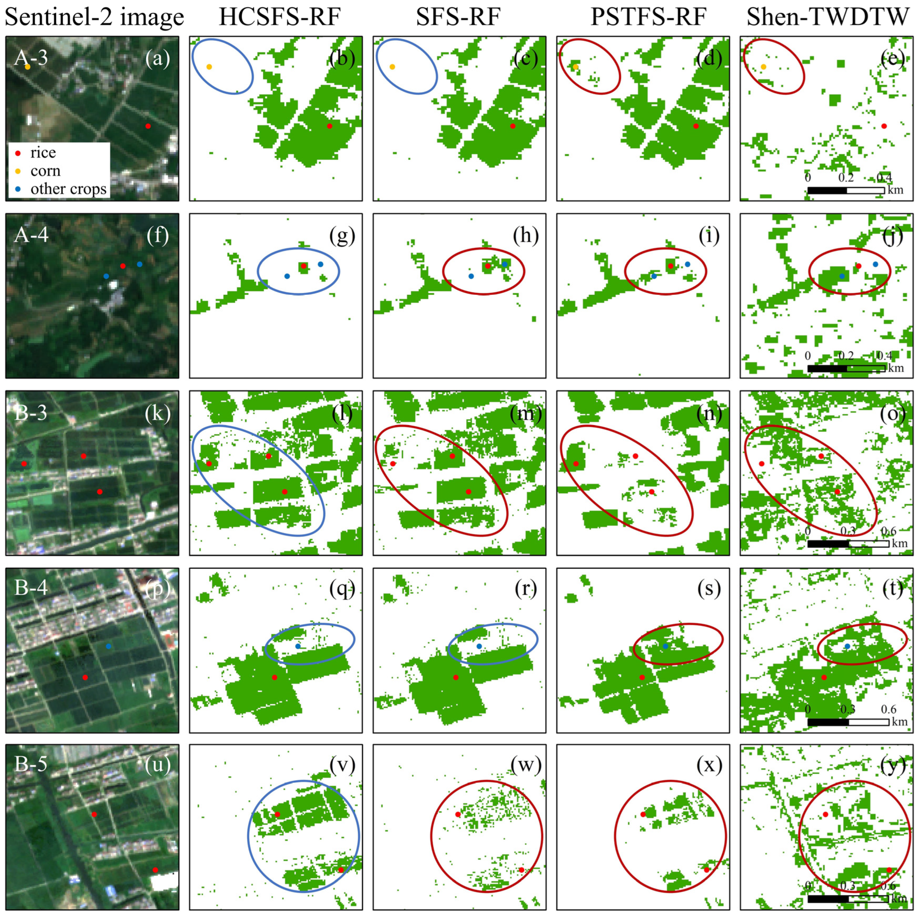
Figure 10 illustrates the classification details of the HCSFS-RF compared with three other rice mapping frameworks introduced in Section 3.3 (SFS-RF, PSTFS-RF, and Shen-TWDTW), for sites A and B. At site A, characterized by complex crop planting structures and fragmented plots, the Shen-TWDTW failed to accurately identify the spatial patterns of rice (Figure 10e,j). While the PSTFS-RF showed better classification performance than the Shen-TWDTW, it still faced challenges in distinguishing corn, other crops, and paddy rice (Figure 10d,i). Furthermore, the primary errors of the SFS-RF lie in its ineffective differentiation of other crops (Figure 10h). At site B, where rice is the predominant land cover type, all four methods effectively identified most of the rice fields. However, the Shen-TWDTW performed poorly in distinguishing rice from other vegetation types (Figure 10o,t,y). The PSTFS-RF not only returned significant omissions but also struggled to differentiate rice from other crops (Figure 10n,s,x). In contrast, the SFS-RF had fewer omissions of rice and no significant misclassification issues (Figure 10m,r,w). Overall, the other three methods in areas with complex topography and planting structures, such as site A, typically exhibited misclassification and low UA (Figure 7a), whereas in areas with relatively sample planting structures, such as site B, they tended to show missed points and low PA (Figure 7d). However, the HCSFS-RF exceled in generating paddy rice maps under varying terrain and climatic conditions, making it more suitable for analyzing real rice cultivation scenarios.
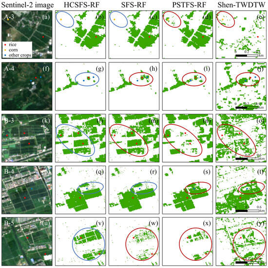
Figure 10.
Comparison of spatial distribution maps of paddy rice acquired using different methods; (a,f,k,p,u) show enlarged views of subsets with true-color composited Sentinel-2 images in the heading period. (b–e, g–j, l–o, q–t, v–y) show enlarged views with the spatial distribution images of rice. The blue and red ellipse boxes represent the correct and error classification, respectively.
4. Discussion
4.1. Transferability of the HCSFS
The robust performance observed at the two sites demonstrates the effective transferability of the HCSFS method across different regions. The factors contributing to the method’s high transferability are (1) the use of a simple clustering parameter determined locally and (2) the superior rice identification performance attained through the integration of classifiers with default parameters.
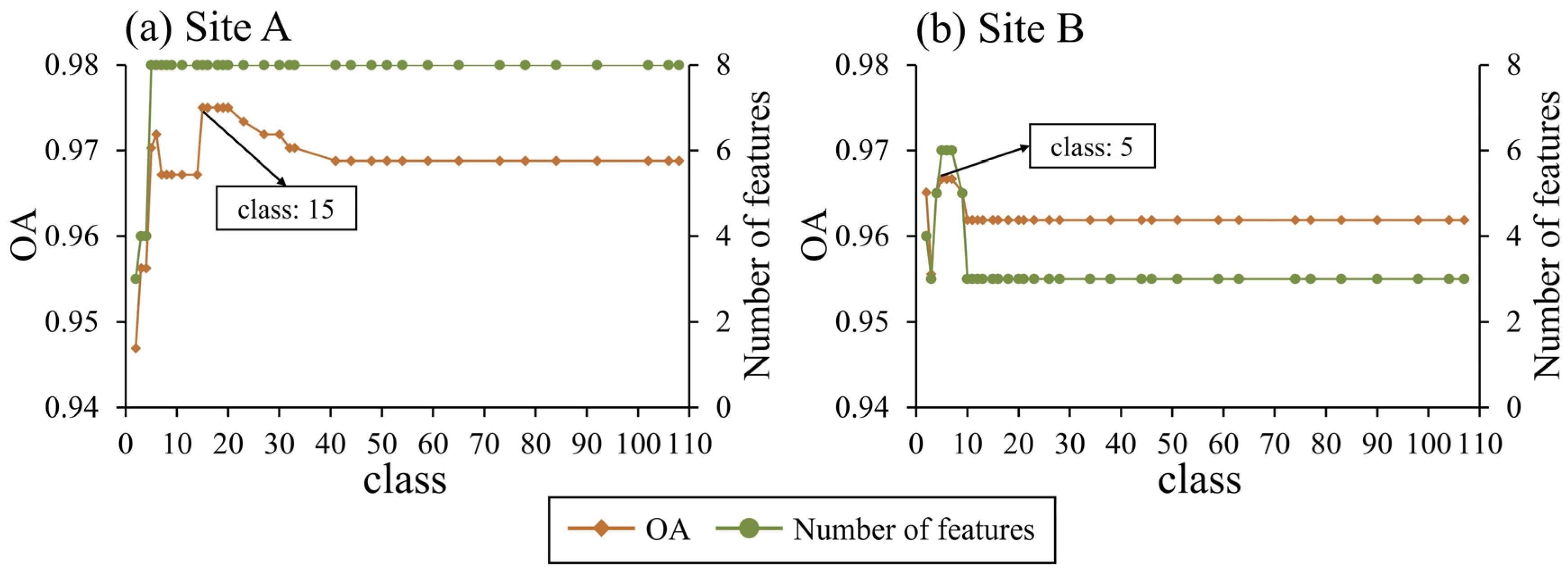
Firstly, the HCSFS method is characterized by a single parameter: the number of classes. Specifically, variations in the number of clusters lead to corresponding changes in the composition of each feature category, thereby producing different optimal feature sets. Investigating the effect of the class number on the quality of the optimal feature set is crucial when using the HCSFS method for feature selection, as the ability of features to distinguish between rice and non-rice significantly affects rice mapping accuracy. To address this issue, we evaluated the performance of the HCSFS-RF framework for rice identification at two research sites with varying numbers of clusters (Figure 11). The results indicated that the HCSFS-RF framework consistently demonstrated excellent identification accuracy (OA > 0.94), regardless of the number of clusters. Specifically, we found that when the number of classes was fewer than five, the number of optimal features selected by the HCSFS was also less than five. Too few features can lead to some important features being discarded, limiting the accuracy of rice mapping. Additionally, when the spectral feature set was divided into 15 classes for feature selection at site A, the framework reached the highest accuracy in rice identification, with an OA of 0.9750. Setting the number of clusters to five produced the highest accuracy at site B, with an OA of 0.9667. However, as the number of classes increased, the OA of the rice mapping initially increased to a peak, then declined with further increases in the number of class, and stabilized when the number of clusters approached half the total number of features. Therefore, when utilizing the HCSFS method to select the optimal feature set for rice identification, it is advisable to keep the number of classes between 5 and 20, ensuring the highest quality of feature set. This guideline can assist users to implement the HCSFS method in other areas.
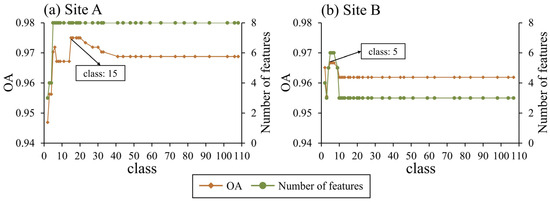
Figure 11.
The OA and feature quantity changes of the HCSFS-RF frameworks under varying numbers of clusters at each study site.
We further computed the execution time for various feature selection methods at the two research sites (Table 4). All methods successfully identified the optimal feature set from the 110 time-series spectral features within two minutes. Among these, the filter methods, especially JM, completed feature selection in the shortest time, due to the absence of training and classification processes. In contrast, the wrapper and embedded methods required more time to identify the optimal feature set for rice. Notably, the proposed HCSFS method did not exhibit a longer execution time than the original SFS. For Site A, HCSFS generated a greater number of feature groups (Figure 11), leading to a reduction in the number of features within each group, thereby enhancing the efficiency of the original SFS method. This finding suggests that the number of features can significantly influence the efficiency of feature selection in wrapper methods.
Table 4.
Execution times (s) required by different feature selection methods.
Secondly, it is widely accepted that feature sets filtered by FS methods are typically input into common RF or SVM classifiers for training to obtain reliable crop classification results, as demonstrated in previous studies [17,21,50]. However, the effectiveness of these FS methods in other advanced machine learning algorithms remains unclear. This study demonstrated that using the optimal feature set selected by HCSFS for rice recognition across nine different classifiers yielded high-quality rice maps, even without advanced hyper-parameter tuning [49] and utilizing only the default parameters provided by Python modules. Due to environmental factors like climate and topography, the spectral characteristics of crops planted in different regions often differ. Whether at site A, characterized by complex terrain, fragmented plots, and diverse crop types, or at site B, featuring simple terrain and intensive rice cultivation, both UA and PA exceeded 0.9548 and 0.9487, respectively (Figure 7). This success can be attributed to the optimal feature set’s remarkable ability to differentiate rice from non-rice across varying terrains and planting structures (Figure 8). This suggests that the HCSFS has the potential to select the optimal feature set for rice mapping in other complex environments. Moreover, the optimal feature set selected by HCSFS shows robust temporal transferability, which can be attributed to the stable and consistent time-series spectral characteristics of crops across different years [56]. The experimental results demonstrate that HCSFS achieves stronger generalization ability by integrating HC and SFS, providing users with more flexible classifier options. In addition, it mitigates the tendency of SFS to fall into local optima and exhibits strong spatial and temporal transferability in rice identification.
4.2. The Applicability of the HCSFS in Early-Season Rice Identification
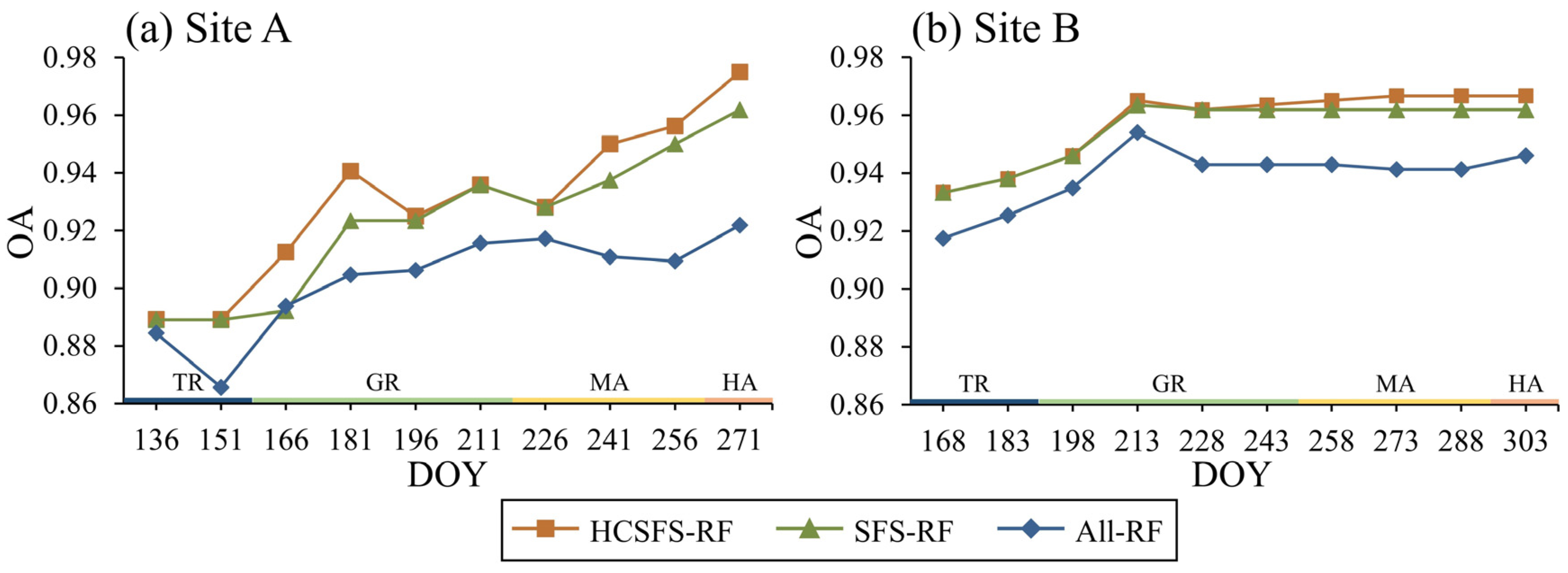
To evaluate the applicability of the HCSFS-RF framework for early recognition, this study tested the rice identification performance of HCSFS-RF, SFS-RF, and All-RF frameworks as the number of time-series images increased, at two research sites with differing climatic conditions and crop planting structures (Figure 12). During the initial two months of the rice growth process, there was a rapid increase in OA as the number of time-series images increased at both Site A and Site B. The HCSFS-RF framework achieved high performance levels (OA > 0.94) during this period at both sites. Compared with the other two frameworks, the HCSFS-RF excels in removing redundancy from the spectral–temporal feature set at all stages, thereby enhancing the accuracy of rice identification.
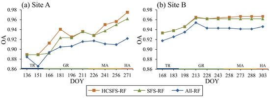
Figure 12.
The OA changes in the HCSFS-RF, SFS-RF, and All-RF frameworks with rice growth: (a) the OA changes at site A in 2022; (b) the OA changes at site B in 2020. All-RF indicates that all features were entered into the RF classifier. TR, GR, MA, and HA represent the transplanting period, growth period, mature period, and harvest period, respectively.
As rice progressed into the maturation and harvesting periods at site A, the classification accuracy of both the HCSFS-RF and SFS-RF frameworks continued to increase rapidly, whereas the All-RF framework showed a relatively slower rate of improvement in accuracy. However, at site B, where the crop planting structures were simpler, the OA of all three frameworks reached a stable state during the rice growth period, with a slight decline in accuracy observed in the All-RF framework. These variations suggest that utilizing spectral–temporal features from multiple phenological stages is particularly beneficial for accurate rice identification in areas with complex planting structures. Figure 8 also reveals that the key features selected by the HCSFS method from the four rice phenological stages at site A were highly distinguishable for rice and non-rice. Moreover, the HCSFS-RF framework was employed to select the optimal feature sets from three early growth period images and one early transplanting period image from Site A and Site B, respectively, resulting in an accurate rice map with OAs exceeding 0.9. This finding is consistent with previous research, which suggests that the transplanting and growth periods of rice are optimal for early identification [2], further confirming the effectiveness of the HCSFS in early rice mapping.
4.3. Limitations of the HCSFS
The HCSFS method effectively removed redundant features from the original spectral feature set, resulting in a rice recognition feature set with regional characteristics and clear differentiation between rice and non-rice. The HCSFS is integrated with various classifiers to generate high-precision rice maps. Experiments conducted in two regions with different planting patterns and climates, as well as early crop identification, demonstrated its temporal and spatial transferability. However, three aspects require improvement to apply this method to larger areas and diverse land cover types. Firstly, the location of rice fields does not remain entirely unchanged over three years, and changes in rice cultivation areas can impact the accuracy of rice recognition. Therefore, we plan to integrate the HCSFS with image fusion technology, leveraging multi-source data such as Landsat, MODIS, and SAR to fill the gaps in Sentinel-2 data [57,58,59], thereby improving the accuracy of rice identification in cloudy regions. Secondly, the mapping results for site A displayed some speckle noise. Due to the site’s hilly terrain, fragmented plots, and complex planting structures, it was challenging to incorporate all land cover types into the training samples. The class imbalance within the training samples significantly impacted the accuracy of the classification results [60], leading to the misclassification of certain pixels as rice. Fortunately, object-based classification methods can reduce speckle noise in the results and improve mapping accuracy [1]. Thus, employing advanced image segmentation algorithms, such as the Segment Anything Model, to scattered pixels in parcel objects before constructing time-series feature sets will become a key research focus in precise rice mapping. Finally, identifying other crops (e.g., corn and soybeans) and rice planting patterns (e.g., double-season rice and triple-season rice) requires the selection of specific time-series spectral feature sets. In future research, we will explore the application of the HCSFS in classifying other crop types and rice planting patterns based on their specific spectral characteristics.
5. Conclusions
This study proposes a new feature selection method, HCSFS, which provides high precision and a compact feature set and is applicable for mapping rice across diverse climates and crop cultivation structures. HCSFS categorizes features and eliminates redundant elements within each category, effectively extracting the optimal spectral and temporal feature set. This approach addresses the local optimality issues of traditional SFS methods, thereby enhancing the accuracy of rice mapping. At two research sites in Sichuan and Jiangsu provinces, we comprehensively evaluated HCSFS and 11 common FS methods using nine widely used machine learning models. The results indicated that among the FS methods, the wrapper method performed better than the embedded method, which in turn performed better than the filter method. The accuracy of HCSFS in different classifiers was better than other methods, with UA greater than 0.9548 and PA greater than 0.9487. Additionally, spatial maps from the two study sites showed that spatial details mapped by HCSFS closely aligned with actual rice cultivation patterns. We anticipate that HCSFS will establish a new paradigm for selecting optimal time-series spectral features and demonstrate its spatial and temporal transferability for mapping rice across broader areas. Future work will focus on developing an annual parcel-level multi-temporal spectral feature set for rice and advancing the application of the HCSFS algorithm in long-term, large-scale rice mapping. Additionally, the application of the HCSFS method to generate high-precision classification maps for other crops and rice planting patterns will be investigated.
Author Contributions
Conceptualization, X.D. and X.W.; methodology, X.D. and X.W.; software, X.D.; validation, X.D., X.W. and X.X.; formal analysis, X.D., X.W. and Q.H.; investigation, X.D., X.W. and Y.C.; resources, X.D. and X.W.; data curation, X.W., J.G., L.D. and L.S.; writing—original draft preparation, X.D.; writing—review and editing, X.D. and X.W.; visualization, X.D.; supervision, X.W., J.G., J.X., X.G. and B.L.; project administration, X.W.; funding acquisition, X.W. All authors have read and agreed to the published version of the manuscript.
Funding
The work was supported by the Natural Resources Research Project of Sichuan Province (No. KJ-2023-6), Financial Fund of Sichuan Institute of Geological Survey (No. SCIGS-CZDXM-2024009), Own funds of Surveying and Mapping Geographic Information Center, Sichuan Institute of Geological Survey (No. SDDY-Z2022006), Deployment project of the Overseas Science and Education Cooperation Center, Bureau of International Cooperation, Chinese Academy of Sciences (No. 162GJHZ2023065MI), and National Undergraduate Innovation and Entrepreneurship Training Program (No. S202310626028).
Institutional Review Board Statement
Not applicable.
Data Availability Statement
The raw data supporting the conclusions of this article will be made available by the authors on request.
Acknowledgments
Firstly, we are very grateful to Google Earth Engine (https://earthengine.google.com/) for their free services, accessed on 1 December 2023. We appreciate the editor and the reviewers for providing valuable suggestions to improve the manuscript.
Conflicts of Interest
The authors declare that they have no conflicts of interest.
References
- Xu, S.; Zhu, X.; Chen, J.; Zhu, X.; Duan, M.; Qiu, B.; Wan, L.; Tan, X.; Xu, Y.N.; Cao, R. A robust index to extract paddy fields in cloudy regions from SAR time series. Remote Sens. Environ. 2023, 285, 113374. [Google Scholar] [CrossRef]
- Gao, Y.; Pan, Y.; Zhu, X.; Li, L.; Ren, S.; Zhao, C.; Zheng, X. FARM: A fully automated rice mapping framework combining Sentinel-1 SAR and Sentinel-2 multi-temporal imagery. Comput. Electron. Agric. 2023, 213, 108262. [Google Scholar] [CrossRef]
- Deng, H.; Zhang, W.; Zheng, X.; Zhang, H. Crop Classification Combining Object-Oriented Method and Random Forest Model Using Unmanned Aerial Vehicle (UAV) Multispectral Image. Agriculture 2024, 14, 548. [Google Scholar] [CrossRef]
- Tian, J.; Tian, Y.; Wan, W.; Yuan, C.; Liu, K.; Wang, Y. Research on the Temporal and Spatial Changes and Driving Forces of Rice Fields Based on the NDVI Difference Method. Agriculture 2024, 14, 1165. [Google Scholar] [CrossRef]
- Dong, J.; Xiao, X.; Menarguez, M.A.; Zhang, G.; Qin, Y.; Thau, D.; Biradar, C.; Moore, B., 3rd. Mapping paddy rice planting area in northeastern Asia with Landsat 8 images, phenology-based algorithm and Google Earth Engine. Remote Sens. Environ. 2016, 185, 142–154. [Google Scholar] [CrossRef] [PubMed]
- Weiss, M.; Jacob, F.; Duveiller, G. Remote sensing for agricultural applications: A meta-review. Remote Sens. Environ. 2020, 236, 111402. [Google Scholar] [CrossRef]
- Xiao, X.; Boles, S.; Liu, J.; Zhuang, D.; Frolking, S.; Li, C.; Salas, W.; Moore, B. Mapping paddy rice agriculture in southern China using multi-temporal MODIS images. Remote Sens. Environ. 2005, 95, 480–492. [Google Scholar] [CrossRef]
- Zheng, B.; Campbell, J.B.; de Beurs, K.M. Remote sensing of crop residue cover using multi-temporal Landsat imagery. Remote Sens. Environ. 2012, 117, 177–183. [Google Scholar] [CrossRef]
- Defourny, P.; Bontemps, S.; Bellemans, N.; Cara, C.; Dedieu, G.; Guzzonato, E.; Hagolle, O.; Inglada, J.; Nicola, L.; Rabaute, T.; et al. Near real-time agriculture monitoring at national scale at parcel resolution: Performance assessment of the Sen2-Agri automated system in various cropping systems around the world. Remote Sens. Environ. 2019, 221, 551–568. [Google Scholar] [CrossRef]
- Zhong, L.; Gong, P.; Biging, G.S. Efficient corn and soybean mapping with temporal extendability: A multi-year experiment using Landsat imagery. Remote Sens. Environ. 2014, 140, 1–13. [Google Scholar] [CrossRef]
- Xiao, X.; Boles, S.; Frolking, S.; Li, C.; Babu, J.Y.; Salas, W.; Moore, B. Mapping paddy rice agriculture in South and Southeast Asia using multi-temporal MODIS images. Remote Sens. Environ. 2006, 100, 95–113. [Google Scholar] [CrossRef]
- Vuolo, F.; Neuwirth, M.; Immitzer, M.; Atzberger, C.; Ng, W.-T. How much does multi-temporal Sentinel-2 data improve crop type classification? Int. J. Appl. Earth Obs. Geoinf. 2018, 72, 122–130. [Google Scholar] [CrossRef]
- Franklin, S.E.; Ahmed, O.S.; Wulder, M.A.; White, J.C.; Hermosilla, T.; Coops, N.C. Large Area Mapping of Annual Land Cover Dynamics Using Multitemporal Change Detection and Classification of Landsat Time Series Data. Can. J. Remote Sens. 2015, 41, 293–314. [Google Scholar] [CrossRef]
- Wang, Z.; Zhang, H.; He, W.; Zhang, L. Cross-phenological-region crop mapping framework using Sentinel-2 time series Imagery: A new perspective for winter crops in China. ISPRS J. Photogramm. Remote Sens. 2022, 193, 200–215. [Google Scholar] [CrossRef]
- Wang, Y.; Zhang, Z.; Feng, L.; Ma, Y.; Du, Q. A new attention-based CNN approach for crop mapping using time series Sentinel-2 images. Comput. Electron. Agric. 2021, 184, 106090. [Google Scholar] [CrossRef]
- Zhang, C.; Zhang, H.; Tian, S. Phenology-assisted supervised paddy rice mapping with the Landsat imagery on Google Earth Engine: Experiments in Heilongjiang Province of China from 1990 to 2020. Comput. Electron. Agric. 2023, 212, 108105. [Google Scholar] [CrossRef]
- Chen, Y.; Hu, J.; Cai, Z.; Yang, J.; Zhou, W.; Hu, Q.; Wang, C.; You, L.; Xu, B. A phenology-based vegetation index for improving ratoon rice mapping using harmonized Landsat and Sentinel-2 data. J. Integr. Agric. 2024, 23, 1164–1178. [Google Scholar] [CrossRef]
- Arvor, D.; Jonathan, M.; Meirelles, M.S.P.; Dubreuil, V.; Durieux, L. Classification of MODIS EVI time series for crop mapping in the state of Mato Grosso, Brazil. Int. J. Remote Sens. 2011, 32, 7847–7871. [Google Scholar] [CrossRef]
- Carrão, H.; Gonçalves, P.; Caetano, M. Contribution of multispectral and multitemporal information from MODIS images to land cover classification. Remote Sens. Environ. 2008, 112, 986–997. [Google Scholar] [CrossRef]
- Löw, F.; Michel, U.; Dech, S.; Conrad, C. Impact of feature selection on the accuracy and spatial uncertainty of per-field crop classification using Support Vector Machines. ISPRS J. Photogramm. Remote Sens. 2013, 85, 102–119. [Google Scholar] [CrossRef]
- Hu, Q.; Sulla-Menashe, D.; Xu, B.; Yin, H.; Tang, H.; Yang, P.; Wu, W. A phenology-based spectral and temporal feature selection method for crop mapping from satellite time series. Int. J. Appl. Earth Obs. Geoinf. 2019, 80, 218–229. [Google Scholar] [CrossRef]
- Ma, Z.; Li, W.; Warner, T.A.; He, C.; Wang, X.; Zhang, Y.; Guo, C.; Cheng, T.; Zhu, Y.; Cao, W.; et al. A framework combined stacking ensemble algorithm to classify crop in complex agricultural landscape of high altitude regions with Gaofen-6 imagery and elevation data. Int. J. Appl. Earth Obs. Geoinf. 2023, 122, 103386. [Google Scholar] [CrossRef]
- Duro, D.C.; Franklin, S.E.; Dubé, M.G. Multi-scale object-based image analysis and feature selection of multi-sensor earth observation imagery using random forests. Int. J. Remote Sens. 2012, 33, 4502–4526. [Google Scholar] [CrossRef]
- Gunal, S.; Edizkan, R. Subspace based feature selection for pattern recognition. Inf. Sci. 2008, 178, 3716–3726. [Google Scholar] [CrossRef]
- Mohamed, S.A.; Metwaly, M.M.; Metwalli, M.R.; AbdelRahman, M.A.E.; Badreldin, N. Integrating Active and Passive Remote Sensing Data for Mapping Soil Salinity Using Machine Learning and Feature Selection Approaches in Arid Regions. Remote Sens. 2023, 15, 1751. [Google Scholar] [CrossRef]
- Zhu, J.; Pan, Z.; Wang, H.; Huang, P.; Sun, J.; Qin, F.; Liu, Z. An improved multi-temporal and multi-feature tea plantation identification method using Sentinel-2 imagery. Sensors 2019, 19, 2087. [Google Scholar] [CrossRef]
- You, N.; Dong, J.; Huang, J.; Du, G.; Zhang, G.; He, Y.; Yang, T.; Di, Y.; Xiao, X. The 10-m crop type maps in Northeast China during 2017–2019. Sci. Data 2021, 8, 41. [Google Scholar] [CrossRef]
- Sánchez-Maroño, N.; Alonso-Betanzos, A.; Tombilla-Sanromán, M. Filter methods for feature selection—A comparative study. In Proceedings of the International Conference on Intelligent Data Engineering and Automated Learning, Birmingham, UK, 16 December 2007; pp. 178–187. [Google Scholar]
- Shafiee, S.; Lied, L.M.; Burud, I.; Dieseth, J.A.; Alsheikh, M.; Lillemo, M. Sequential forward selection and support vector regression in comparison to LASSO regression for spring wheat yield prediction based on UAV imagery. Comput. Electron. Agric. 2021, 183, 106036. [Google Scholar] [CrossRef]
- Marcano-Cedeño, A.; Quintanilla-Domínguez, J.; Cortina-Januchs, M.; Andina, D. Feature selection using sequential forward selection and classification applying artificial metaplasticity neural network. In Proceedings of the IECON 2010—36th Annual Conference on IEEE Industrial Electronics Society, Glendale, AZ, USA, 7–10 November 2010; pp. 2845–2850. [Google Scholar]
- Haq, A.U.; Li, J.; Memon, M.H.; Memon, M.H.; Khan, J.; Marium, S.M. Heart disease prediction system using model of machine learning and sequential backward selection algorithm for features selection. In Proceedings of the 2019 IEEE 5th International Conference for Convergence in Technology (I2CT), Bombay, India, 29–31 March 2019; pp. 1–4. [Google Scholar]
- Vince, A. A framework for the greedy algorithm. Discret. Appl. Math. 2002, 121, 247–260. [Google Scholar] [CrossRef]
- Ni, R.; Tian, J.; Li, X.; Yin, D.; Li, J.; Gong, H.; Zhang, J.; Zhu, L.; Wu, D. An enhanced pixel-based phenological feature for accurate paddy rice mapping with Sentinel-2 imagery in Google Earth Engine. ISPRS J. Photogramm. Remote Sens. 2021, 178, 282–296. [Google Scholar] [CrossRef]
- Shen, R.; Pan, B.; Peng, Q.; Dong, J.; Chen, X.; Zhang, X.; Ye, T.; Huang, J.; Yuan, W. High-resolution distribution maps of single-season rice in China from 2017 to 2022. Earth Syst. Sci. Data. 2023, 2023, 1–27. [Google Scholar] [CrossRef]
- Griffiths, P.; Nendel, C.; Hostert, P. Intra-annual reflectance composites from Sentinel-2 and Landsat for national-scale crop and land cover mapping. Remote Sens. Environ. 2019, 220, 135–151. [Google Scholar] [CrossRef]
- Liu, L.; Xiao, X.; Qin, Y.; Wang, J.; Xu, X.; Hu, Y.; Qiao, Z. Mapping cropping intensity in China using time series Landsat and Sentinel-2 images and Google Earth Engine. Remote Sens. Environ. 2020, 239, 111624. [Google Scholar] [CrossRef]
- Tucker, C.J. Red and Photographic Infrared Linear Combinations for Monitoring Vegetation. Remote Sens. Environ. 1978, 8, 127–150. [Google Scholar] [CrossRef]
- Huete, A.R.; Liu, H.Q.; Batchily, K.; van Leeuwen, W. A Comparison of Vegetation Indices over a Global Set of TM Images for EOS-MODIS. Remote Sens. Environ. 1997, 59, 440–451. [Google Scholar] [CrossRef]
- Johnson, S.C. Hierarchical clustering schemes. Psychometrika 1967, 32, 241–254. [Google Scholar] [CrossRef] [PubMed]
- Zhang, L.; Zhong, Y.; Huang, B.; Gong, J.; Li, P. Dimensionality Reduction Based on Clonal Selection for Hyperspectral Imagery. IEEE Trans. Geosci. Remote Sens. 2007, 45, 4172–4186. [Google Scholar] [CrossRef]
- Gao, S.; Tang, B.-H.; Huang, L.; Chen, G. Identification of tea plantations in typical plateau areas with the combination of Sentinel-1/2 optical and radar remote sensing data based on feature selection algorithm. Int. J. Remote Sens. 2023, 1–21. [Google Scholar] [CrossRef]
- Ashourloo, D.; Nematollahi, H.; Huete, A.; Aghighi, H.; Azadbakht, M.; Shahrabi, H.S.; Goodarzdashti, S. A new phenology-based method for mapping wheat and barley using time-series of Sentinel-2 images. Remote Sens. Environ. 2022, 280, 113206. [Google Scholar] [CrossRef]
- Chen, X.; Yang, K.; Ma, J.; Jiang, K.; Gu, X.; Peng, L. Aboveground Biomass Inversion Based on Object-Oriented Classification and Pearson–mRMR–Machine Learning Model. Remote Sens. 2024, 16, 1537. [Google Scholar] [CrossRef]
- Yin, L.; You, N.; Zhang, G.; Huang, J.; Dong, J. Optimizing Feature Selection of Individual Crop Types for Improved Crop Mapping. Remote Sens. 2020, 12, 162. [Google Scholar] [CrossRef]
- Cao, Y.; Dai, J.; Zhang, G.; Xia, M.; Jiang, Z. Combinations of Feature Selection and Machine Learning Models for Object-Oriented “Staple-Crop-Shifting” Monitoring Based on Gaofen-6 Imagery. Agriculture 2024, 14, 500. [Google Scholar] [CrossRef]
- Jin, M.; Xu, Q.; Guo, p.; Han, B.; Jin, J. Crop classification method from UAV images based on Object-Oriented Multi-feature Learning. Remote Sens. Technol. Appl. 2023, 38, 588–598. [Google Scholar] [CrossRef]
- Tian, Y.; Shuai, Y.; Shao, C.; Wu, H.; Fan, L.; Li, Y.; Chen, X.; Narimanov, A.; Usmanov, R.; Baboeva, S. Extraction of Cotton Information with Optimized Phenology-Based Features from Sentinel-2 Images. Remote Sens. 2023, 15, 1988. [Google Scholar] [CrossRef]
- Zhang, K.; Chen, Y.; Zhang, B.; Hu, J.; Wang, W. A Multitemporal Mountain Rice Identification and Extraction Method Based on the Optimal Feature Combination and Machine Learning. Remote Sens. 2022, 14, 5096. [Google Scholar] [CrossRef]
- Li, H.; Song, X.-P.; Hansen, M.C.; Becker-Reshef, I.; Adusei, B.; Pickering, J.; Wang, L.; Wang, L.; Lin, Z.; Zalles, V.; et al. Development of a 10-m resolution maize and soybean map over China: Matching satellite-based crop classification with sample-based area estimation. Remote Sens. Environ. 2023, 294, 113623. [Google Scholar] [CrossRef]
- Luo, K.; Lu, L.; Xie, Y.; Chen, F.; Yin, F.; Li, Q. Crop type mapping in the central part of the North China Plain using Sentinel-2 time series and machine learning. Comput. Electron. Agric. 2023, 205, 107577. [Google Scholar] [CrossRef]
- Wang, X.; Zhang, J.; Xun, L.; Wang, J.; Wu, Z.; Henchiri, M.; Zhang, S.; Zhang, S.; Bai, Y.; Yang, S. Evaluating the effectiveness of machine learning and deep learning models combined time-series satellite data for multiple crop types classification over a large-scale region. Remote Sens. 2022, 14, 2341. [Google Scholar] [CrossRef]
- Woźniak, E.; Rybicki, M.; Kofman, W.; Aleksandrowicz, S.; Wojtkowski, C.; Lewiński, S.; Bojanowski, J.; Musiał, J.; Milewski, T.; Slesiński, P. Multi-temporal phenological indices derived from time series Sentinel-1 images to country-wide crop classification. Int. J. Appl. Earth Obs. Geoinf. 2022, 107, 102683. [Google Scholar] [CrossRef]
- Yang, L.; Mansaray, L.R.; Huang, J.; Wang, L. Optimal segmentation scale parameter, feature subset and classification algorithm for geographic object-based crop recognition using multisource satellite imagery. Remote Sens. 2019, 11, 514. [Google Scholar] [CrossRef]
- Foody, G.M. Status of land cover classification accuracy assessment. Remote Sens. Environ. 2002, 80, 185–201. [Google Scholar] [CrossRef]
- Congalton, R.G. A review of assessing the accuracy of classifications of remotely sensed data. Remote Sens. Environ. 1991, 37, 35–46. [Google Scholar] [CrossRef]
- You, N.; Dong, J. Examining earliest identifiable timing of crops using all available Sentinel 1/2 imagery and Google Earth Engine. ISPRS J. Photogramm. Remote Sens. 2020, 161, 109–123. [Google Scholar] [CrossRef]
- Zhao, Y.; Huang, B.; Song, H. A robust adaptive spatial and temporal image fusion model for complex land surface changes. Remote Sens. Environ. 2018, 208, 42–62. [Google Scholar] [CrossRef]
- Zhu, X.; Helmer, E.H.; Gao, F.; Liu, D.; Chen, J.; Lefsky, M.A. A flexible spatiotemporal method for fusing satellite images with different resolutions. Remote Sens. Environ. 2016, 172, 165–177. [Google Scholar] [CrossRef]
- Zhao, R.; Li, Y.; Chen, J.; Ma, M.; Fan, L.; Lu, W. Mapping a Paddy Rice Area in a Cloudy and Rainy Region Using Spatiotemporal Data Fusion and a Phenology-Based Algorithm. Remote Sens. 2021, 13, 4400. [Google Scholar] [CrossRef]
- Heydari, S.S.; Mountrakis, G. Effect of classifier selection, reference sample size, reference class distribution and scene heterogeneity in per-pixel classification accuracy using 26 Landsat sites. Remote Sens. Environ. 2018, 204, 648–658. [Google Scholar] [CrossRef]


Disclaimer/Publisher’s Note: The statements, opinions and data contained in all publications are solely those of the individual author(s) and contributor(s) and not of MDPI and/or the editor(s). MDPI and/or the editor(s) disclaim responsibility for any injury to people or property resulting from any ideas, methods, instructions or products referred to in the content. |
© 2024 by the authors. Licensee MDPI, Basel, Switzerland. This article is an open access article distributed under the terms and conditions of the Creative Commons Attribution (CC BY) license (https://creativecommons.org/licenses/by/4.0/).