Predicting Vase Life of Cut Lisianthus Based on Biomass-Related Characteristics Using AutoML

Abstract

Lisianthus, a globally popular ornamental plant, has a variable vase life (5–28 days). This study investigated biomass-related characteristics of four cultivars grown in soil or hydroponic cultivation with different treatment timings (vegetative and reproductive stage) and concentrations (0, 0.1, 0.3, and 0.5 mM) of salicylic acid (SA) in order to explain vase life. The results show that the SA treatment effects varied depending on cultivar, SA treatment timing, concentration, and cultivation method. Principle component analysis revealed that Blue Picote cultivar cultivated hydroponically with 0.5 mM SA at the reproductive stage had the longest vase life. Furthermore, vase life demonstrated a high positive correlation with dry weight, SPAD, Mg content, and flowering day. We developed a model using automated machine learning algorithms to estimate postharvest vase life, based on biomass-related characteristics measured during the pre-harvest period. Similar to the PCA results, this model also identified dry weight as the most influential predictor of vase life. This model proposes the possibility of estimating vase life by setting characteristics highly correlated with vase life as features for machine learning. It is anticipated that this model will be widely utilized in the floriculture industry for standardizing cut flower quality assessments in the future.

1. Introduction

Lisianthus (Eustoma grandiflorum) is a herbaceous flowering plant from the Gentianaceae family and has been cultivated since 1960 [1]. It blooms uniformly throughout the year, has a shape and size similar to that of roses, and blooms in a variety of colors. Cut lisianthus flowers are gaining popularity both for their versatility in design and for the ease of transportation worldwide. For over 20 years, several studies have tried to improve the vase life of cut lisianthus [2,3,4,5].

Post-harvest longevity varies extremely between 5–9 and 28 days depending on the cultivar or cultivation method [5,6,7,8,9]. Recently, the timing and concentration of salicylic acid (SA) treatment and cultivation method have been shown to influence the vase life of cut lisianthus [10]. Among the various experimental conditions, SA treatment was most beneficial when applied during the reproductive period at a 0.5 mM concentration with hydroponics. Moreover, Kroma White (KW) cultivar lived up to 19 days under the aforementioned conditions. In fact, the use of a machine learning (ML) model with colorimetric data provided a better predictive performance of vase life (r² = 0.96) than that of SPAD data (r² = 0.70).

Plant growth is defined as an increase in biomass, which can be measured using biometric parameters such as dry weight, stem height, and leaf area [11]. Stem development in crops is an important factor affecting crop growth, yield, and agricultural characteristics [12]. Generally, the thicker the stem diameter, the longer the vase life of the cut flower. The vase life of cut flowers correlates with the diameter and strength of the stem because thicker stems may have larger vascular bundles that increase efficient water and nutrient transport [13], and may be less prone to air embolism caused by small air bubble-induced obstructions of vertical water flow into the stem [14]. Additionally, stem length is an important factor in determining the quality and productivity of cut flowers. Therefore, stem length is used for quality grading in the marketing of cut roses [13].

Plant growth regulators affect plant height, length of flowers or inflorescence stems, flower size, and number of leaves. Additionally, they improve plant quality, flowering intensity, and flower vase life [15]. SA treatment promotes photosynthetic efficiency, which in turn increases plant biomass [16]. Specifically, the SA analog benzothiadiazole improves both disease resistance and fresh weight [17]. SA treatment improved photosynthesis and stomatal conductance in Achillea millefolium [18] and improved photosynthesis in Centella asiatica [19]. In addition to SA treatment, various chemical treatments promote the post-harvest longevity of cut flowers with increased biomass [8,9,20,21,22,23], flower fresh matter weight, flower diameter, and flower opening time [24]. The fresh weight and vase life of sampaguita (Jasminum sambac) increased on foliar chemical application [20]. Aluminum sulfate and sucrose application extended the vase life of lilium flowers up to 18 days by increasing flower diameter, flower fresh weight, and spike length, and delaying maximum floret opening and flower opening time [23]. Increasing the nitrogen level through ammonium (NH₄⁺) application improves a number of growth parameters in lisianthus, including height; number of flowers and leaves; leaf area; and shoot, stem, and leaf dry weight [25].

Pre-harvest plant growth conditions exert an approximately 30–70% effect on cut flower quality [26]. Therefore, appropriate treatments are useful in promoting preharvest growth conditions to increase the vase life of cut flowers. In this study, we investigated four lisianthus cultivars to address the following questions: (1) which biomass-related characteristics, namely, vegetative (stem diameter, number of stem nodes, stem length, number of stem bushes, flowering day, and SPAD value), reproductive (fresh weight, dry weight, weight difference, petal number, petal size), and leaf chemical components (nitrogen (N), phosphorus (P), potassium (K), magnesium (Mg), and calcium (Ca)), are affected by SA treatment concentration, treatment timing, and cultivation method? (2) Which of the characteristics are associated with the longevity of cut flowers? Additionally, principal component analysis (PCA) was employed to identify the optimal conditions for maximizing vase life based on the factors considered in this experiment: cultivar, SA treatment timing, concentration, and cultivation method. We followed the explanatory analyses with (3) a predictive analysis using ML algorithms based on biomass-related characteristics as predictors of vase life of cut lisianthus. The specific hypotheses that were tested have been mentioned in Section 2.7 (Statistical analysis). We found that the hydroponic cultivation of Blue Picote (BP) cultivar with 0.5 mM SA at the reproductive stage exhibited the longest vase life. Moreover, both PCA and ML analyses showed that dry weight was the strongest predictor of vase life.

2. Materials and Methods

2.1. Plant Materials

Seedlings of the four lisianthus cultivars, namely, Arena Green (AG), Blue Picote (BP), Corelli Pink (CP), and Kroma White (KW), were planted in the greenhouse at the Pocheon Agricultural Technology Center on 22 June 2022. These cultivars are known for their variety in colors and are popular in the current market. The lisianthus shipments were strategically timed to align with holidays to capitalize on the increased demand for flowers during such periods.

Lisianthus is a captivate consumer, and the growth parameters described in this section were maintained in the greenhouse throughout the cultivation period. To accelerate the flowering process, lisianthus plants were cultivated at temperatures that were higher than the optimal growth range. An average temperature of 28 °C was maintained during the day and 22 °C at night, which exceeded the recommended ranges of 24–26 °C (day) and 15–18 °C (night). The average light duration was 13.5 h; natural daylight was provided with shading from 11:00 a.m. to 2:00 p.m. on days of high light intensity or artificial light on cloudy days. The humidity level was 65 ± 10%, and CO₂ concentration was 393.3 ppm.

The soil mixture used for soil cultivation comprised peat moss, horticultural substrates, perlite, and oil cake in the following proportions: 0.50:0.38:0.10:0.02. Composite soil samples analysis showed the following parameters: pH (1:5), 6.9; organic matter (OM), 54 g kg⁻¹; available phosphate (Av. P₂O₄), 790 mg kg⁻¹; exchangeable (Exch.) K, 14.8 cmol_c kg⁻¹; Exch. Ca, 14.8 cmol_c kg⁻¹; Exch. Mg, 4.8 cmol_c kg⁻¹; and electrical conductivity (EC), 2.3 dS m⁻¹.

A four-element compound fertilizer, namely, BioNex liquid fertilizer (N (5.1%), P (10), K (5), and micronutrients; Bio Trading, Busan, Republic of Korea), was sprayed on the leaves 40 days after planting at the dose of 30 mL/application. Additionally, the CalBungMa fertilizer (Ca (15.5%), N (5), B (0.1), and Mg (4.1); KoreaAgro, Chungbuk, Republic of Korea) was sprayed on the leaves 50 days after planting at the dose of 30 mL/application. The fertilizer standard solution was diluted in 12 L of water and applied evenly to the foliage using a semi-automatic sprayer.

A 1000 L nutrient solution was prepared for tank A by combining KNO₃ (303 g), CaNO₃ (944 g), and Fe-EDTA (22.62 mg). The same volume of nutrient solution was prepared for Tank B by combining KNO₃ (303 g), NH₄H₂PO₄ (115 g), MgSO₄·7H₂O (492 g), CuSO₄·5H₂O (78.58 mg), H₃BO₃ (2858.5 mg), MnSO₄·H₂O (1538 mg), ZnSO₄·7H₂O (219.8 mg), and NH₄Mo₇O₂₄·4H₂O (121.3 mg). The nutrient solutions were applied using a drip irrigation system. Nutrient solution analysis showed the following parameters: pH (1:5), 6.7; OM, 54 g kg⁻¹; Av. P₂O₄, 674 mg kg⁻¹; Exch. K, 13.7 cmol_c kg⁻¹; Exch. Ca, 13.7 cmol_c kg⁻¹; Exch. Mg, 4.4 cmol_c kg⁻¹; and EC, 2.7 dS m⁻¹. The growth medium contained peat moss and perlite in a 1:1 ratio.

Designated beds were established for hydroponic and soil cultivation. In total, 1000 lisianthus seedlings were randomly allocated to either the soil cultivation or hydroponic cultivation groups. Both cultivation groups were treated in identical greenhouses with only the moisture and nutrient content of the soil varying. In the soil cultivation group, lisianthus was planted in containers measuring 35 × 30 × 24 cm in groups of three. During the initial 2 weeks post-planting, each container was provided with 2 L of water four times per week. From week 3, the same quantity of water was provided thrice weekly. The watering regimen was maintained consistently between 9:00 a.m. and 10:00 a.m. In the hydroponic cultivation group, lisianthus plants were replanted in 30 × 40 × 2500 cm containers filled with a growing medium. Only tap water was supplied during the initial 2 weeks post-planting. On week 3, 30 mL of the nutrient solution was provided five times a day at 10 s durations using the drip irrigation system. From week 4, 40 mL of the nutrient solution was provided eight times a day at 10 s durations. Consequently, the plants in the soil cultivation group occupied a smaller area compared with those of the hydroponic cultivation group, and the two cultivation groups received different levels of moisture and nutrients. Following cultivation, six samples were randomly selected for analysis in each treatment, and this procedure was repeated thrice for both groups.

The first flower bloom occurred at 56 days in the soil cultivation group and 58 days in the hydroponic cultivation group. The relatively earlier flowering in the soil cultivation group may be attributed to inadequate nutrition and drought stress [27]. Furthermore, more time was required to harvest three flowers from each lisianthus plant in the hydroponic cultivation group than in the soil cultivation group.

2.2. Soil or Hydroponic Cultivation at Vegetative or Reproductive Period

Hormonal treatment was applied either at the vegetative (V) or reproductive (R) stage. Stage V was defined as 3 weeks after lisianthus seedlings developed roots during stages 1, 2, and 3 post-planting. The R stage was defined as the period of SA treatment starting at flower bud development when approximately 60–70% of flower budding occurred in the average plant. SA (Gooworl Co., Daegu, Republic of Korea) was dissolved in methanol as a 100-fold concentrate and diluted with water for application. Six samples from each group were subjected to SA treatment. The experimental concentrations were 0, 0.1, 0.3, and 0.5 mM. For each SA concentration, 10 mL was applied thrice at 3-day intervals between 10:00 a.m. and 12:00 p.m.. The control group received 10 mL of tap water. SA was applied 7 weeks after lisianthus planting for the soil cultivation group and 8 weeks after planting for the hydroponic cultivation group. However, a 7-day discrepancy was observed in SA application because of the differences in the bloom timing between the soil and hydroponic cultivation groups.

2.3. Measurement of Vegetative Characteristics

Vegetative characteristics, namely, stem diameter (mm), stem node (no.), stem length (mm), stem bush (no.), flowering day (day), and SPAD (value), were measured in this study. Stem diameter was measured in terms of growth after planting at the fourth or fifth node from the bottom. Chlorophyll content was measured during stage V using a chlorophyll meter MC-100 (Apogee Instruments, North Logan, UT, USA). As the leaf locations differed for each cultivar, measurements were taken only from leaves where the lateral branches started forming Y shapes to ensure consistency.

2.4. Measurement of Reproductive Characteristics

To investigate flower characteristics, flowers were cut on 31 August 2022 for the S cultivation groups (68 days) and 16 September 2022 for the H cultivation groups (83 days). Considering factors such as flower size and flower opening (that is, the flower was 60–70% open), we selected and cut flowers that had bloomed to a similar degree. The measured reproductive characteristics were fresh weight (mg), dry weight (mg), weight difference (mg), vase life (days), petal number (no.), petal size (mm), and petal color (CIELAB value). Lisianthus cultivars showed differences in flowers, stems, and appearance and location of leaves; hence, the flower stems were cut to 5 cm-long segments to create equal conditions. All lower leaves were removed. Fresh weight was measured as biomass on the day of measurement, and dry weight was measured in the dry state after flower cutting. Weight difference was calculated by subtracting the dry weight from the fresh weight. Vase life was measured in a laboratory at a constant temperature of 20.4 °C, relative humidity of 60–76%, and illumination of 7.43–9.45 µmol m² s⁻¹. The vase life of each sample was defined as the time at which an investigator observed a change in the petal color and the collapse of the petal shape. Petal number, size, and color were examined on the first day after flower cutting. Petal color was measured using a colorimeter (CR-300; Konica Minolta, Tokyo, Japan) and was only used for PCA.

2.5. Leaf Chemical Analysis of Cut Lisianthus

Leaves were collected from each group on the day of cutting to measure the concentrations of the accumulated inorganic compounds, namely, N, P, K, Mg, and Ca. Next, 0.5 g of leaves from the cut plants were dried completely for 8 h at 70 °C and homogenized using a miniature homogenizer. The sample (three replicates) was digested in the 10 mL reagent mixture (distilled water (DW) 1000 mL + 1800 mL of 50% perchloric acid + 200 mL of 30% sulfuric acid) using a heating block at 25 °C for 8 h and 200 °C for 8 h. After the solution cooled to below 60 °C, an aliquot was diluted with DW in 100 mL mess flasks and filtered using Whatman No. 6 filter paper. Total N level was analyzed using the Kjeldahl method [28], and P level was analyzed using the Vanadate method [29]. K, Mg, and Ca levels were analyzed using inductively coupled plasma–optical emission spectrometry (Integra XL ICP-OES, GBC Scientific Equipment, Victoria, Australia). The concentrations of all chemicals were expressed as mg g⁻¹ of dry weight.

2.6. Study Groups

Biomass-related characteristics of the AG, BP, CP, and KW cultivars were investigated at different SA concentrations (0, 0.1, 0.3, or 0.5 mM) in four treatment groups that were established based on the combination of cultivation method (soil or hydroponic cultivation) and SA treatment timing (vegetative or reproductive period). The groups were SSV (soil cultivation, SA treatment, and vegetative stage), SSR (soil cultivation, SA treatment, and reproductive stage), HSV (hydroponics, SA treatment, and vegetative stage), and HSR (hydroponics, SA treatment, and reproductive stage). Hereafter, H cultivation group refers to the combined HSV and HSR groups, and S cultivation refers to the combined SSV and SSR groups.

2.7. Statistical Analysis

We hypothesized that the effect of SA treatment on biomass-related characteristics depends on the cultivation method and treatment timing. We further assumed that the effects were cultivar-specific. Therefore, we analyzed the interaction of SA treatment concentration (0, 0.1, 0.3, and 0.5 mM) and treatment group (SSV, SSR, HSV, and HSR) for each cultivar using the two-way ANOVA. Hypothesis testing was performed at a significance level of 0.05, and the p-values were adjusted for multiple tests [30]. To identify the individual characteristics associated with the vase life of cut flowers, we used negative binomial regression to account for potential overdispersion in vase life. The p-values were adjusted for multiple tests [30].

For the second objective, we tried to find the characteristics that were most correlated with vase life. PCA was performed using “magrittr”, “FactoMineR”, and “factoextra” packages in R version 4.4.1.

Finally, ML algorithms were used to predict vase life (days) using biomass-related characteristics. Root mean square error (RMSE), mean average error (MAE), and R-square (R²) were calculated to evaluate and compare the predictive performances of the ML algorithms. The “h2o” and “lares” packages were used to implement the ML algorithms in R [31,32].

3. Results

3.1. Vase Life

We set the vase life of the post-harvest period as the target variable and investigated the vegetative and reproductive characteristics and leaf chemical components of the pre-harvest period. Based on these traits, we performed a correlation analysis with vase life, PCA, and a machine learning model to predict vase life. The effects of four environmental conditions and four SA concentrations (management) on the vase life of the four cultivars have been reported in our previous studies [10]. Therefore, this study did not include results analyzing vase life as a characteristic. This study serves as a follow-up to our previous research, and its results can be compared with previous research findings [10].

3.2. Vegetative Characteristics

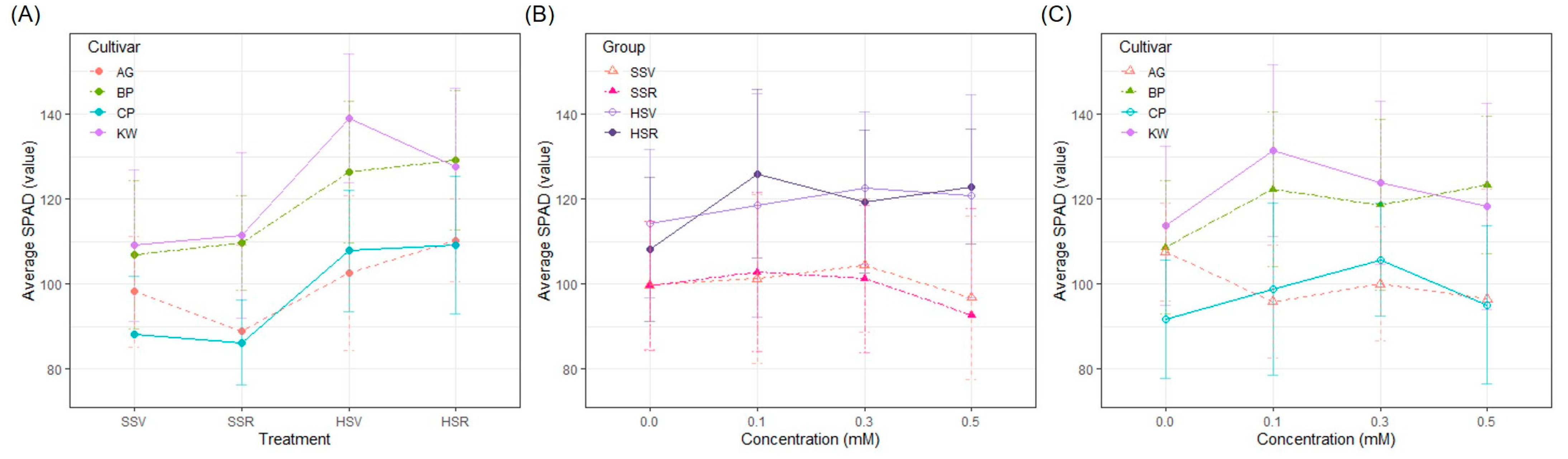
The characteristics investigated during the vegetative period included stem diameter, stem nodes, stem length, stem bushes, flowering day, and SPAD value. Among the various vegetative characteristics, SPAD value exhibited the highest correlation with vase life (r = 0.329) (Figure S1). Therefore, only SPAD is discussed in detail within this section. With the exception of the SPAD values, all characteristics are presented in the Supplementary Data. Graphs have been provided for each characteristic with respect to SA treatment concentration, cultivation method, timing, and cultivar in Figures S1–S6, included in the Supplementary Data.

SPAD Value

SPAD values estimate the chlorophyll content and potential photosynthetic efficiency of leaves as indirect indicators [33]. The SPAD values differed significantly depending on treatment group, cultivar (p < 0.001), and SA concentration (p < 0.05) (Figure 1). The average SPAD value was higher in the H cultivation group than in the S cultivation group, and was not affected by SA concentration. The BP and KW cultivars showed significantly higher average SPAD values than those of the AG and CP cultivars in all treatments. The SPAD value is highly influenced by the genotype; therefore, the trend of the SPAD value of each cultivar remained the same, despite changes in the environment. The highest correlation coefficient with vase life was shown by SPAD value (r = 0.329) among the vegetative characteristics and by BP (r = 0.434) among the four cultivars (Figure S2).

3.3. Reproductive Characteristics

Among the reproductive characteristics, dry weight correlated most highly with vase life (Figure 2). All other characteristics are described in the Supplementary Data (Figures S7–S10).

Dry Weight

Among the reproductive characteristics, dry weight correlated most highly with vase life (r = 0.508). The KW (r = 0.687) and BP (r = 0.632) cultivars showed the highest correlation coefficients, suggesting that dry weight is the most important factor in classifying vase life. There was a low correlation between fresh weight and vase life (r = 0.154). However, fresh weight showed strong correlation with weight difference (r = 0.708). Based on cultivar, CP (r = 0.654) and BP (r = 0.808) showed strong correlations with these two variables, which could be attributed to the tissue’s high water content in both cultivars. In contrast, AG and KW showed a weak-to-moderate relationship, indicating relatively low water content. Moreover, dry weight and weight difference showed a moderately negative correlation (r = −0.448). Additionally, weight difference and vase life showed a weak negative correlation (r = −0.234).

Figure 3 shows that the average dry weight of the HSR group was significantly higher than those of the other treatment groups. Particularly, the KW cultivar in the HSR group showed the highest average dry weight of 2.38 g. Dry weight was significantly affected by the treatment group, cultivar, and their interaction (

Table 1. Treatment effects on each characteristic by cultivar. *, **, and *** implying p < 0.05, p < 0.01, and p < 0.001, respectfully.

	AG			BP			CP			KW
Characteristic	A	B	A × B	A	B	A × B	A	B	A × B	A	B	A × B
Stem diameter	0.024 *	0.810	0.616	0.001 **	0.571	0.017 *	0.021 *	0.043*	<0.001 ***	0.019 *	0.469	0.725
Stem node	<0.001 ***	0.039 *	0.223	0.002 **	0.993	0.504	0.007 **	0.202	0.668	0.001 **	0.078	0.095
Stem length	<0.001 ***	0.352	0.599	0.036 *	0.279	0.420	<0.001 ***	0.048 *	0.316	<0.001 ***	0.209	0.618
Stem bush	<0.001 ***	0.054	0.397	<0.001 ***	0.962	0.026 *	<0.001 ***	0.039 *	0.202	<0.001 ***	0.118	0.092
Flowering day	0.018 *	0.040 *	0.187	0.215	0.001 **	0.047 *	<0.001 ***	<0.001 ***	0.165	0.124	0.042 *	0.104
SPAD	<0.001 ***	0.057	0.410	<0.001 ***	0.007 **	0.615	<0.001 ***	<0.001 ***	0.001 **	<0.001 ***	0.007 **	0.739
Nitrogen	<0.001 ***	<0.001 ***	<0.001 ***	<0.001 ***	<0.001 ***	<0.001 ***	<0.001 ***	<0.001 ***	<0.001 ***	<0.001 ***	<0.001 ***	<0.001 ***
Phosphorus	<0.001 ***	<0.001 ***	<0.001 ***	<0.001 ***	<0.001 ***	<0.001 ***	<0.001 ***	<0.001 ***	<0.001 ***	<0.001 ***	<0.001 ***	<0.001 ***
Potassium	<0.001 ***	<0.001 ***	<0.001 ***	<0.001 ***	<0.001 ***	<0.001 ***	<0.001 ***	<0.001 ***	<0.001 ***	<0.001 ***	<0.001 ***	<0.001 ***
Calcium	<0.001 ***	<0.001 ***	<0.001 ***	<0.001 ***	<0.001 ***	<0.001 ***	<0.001 ***	0.275	<0.001 ***	<0.001 ***	<0.001 ***	<0.001 ***
Magnesium	<0.001***	<0.001 ***	<0.001 ***	<0.001 ***	<0.001 ***	0.055	<0.001 ***	<0.001 ***	<0.001 ***	<0.001 ***	<0.001 ***	<0.001 ***
Fresh weight	<0.001 ***	0.352	0.352	<0.001 ***	0.807	0.463	<0.001 ***	0.104	0.458	0.292	0.871	0.23
Dry weight	<0.001 ***	0.749	0.810	<0.001 ***	0.555	0.783	<0.001 ***	0.007 **	<0.001 ***	<0.001 ***	0.351	0.223
Weight difference	<0.001 ***	0.024 *	0.247	<0.001 ***	0.439	0.393	0.002 **	0.007 **	0.115	<0.001 ***	0.505	0.306
Petals	0.616	0.625	0.893	<0.001 ***	0.381	0.051	<0.001 ***	0.48	0.345	0.739	<0.001 ***	0.464
Petal size	<0.001 ***	0.424	<0.001 ***	<0.001 ***	<0.001 ***	0.504	<0.001 ***	0.304	0.234	<0.001 ***	0.061	0.004 **

AG, Arena Green; BP, Blue Picote; CP, Corelli Pink; KW, Kroma White; SPAD, soil plant analysis development; A = treatment group; B = concentration; and A × B = interaction. p-values of two-way ANOVA are adjusted for multiple tests.

). Dry weight increased substantially for the H cultivation compared with that of the S cultivation. Compared to the average in the SSR group, the HSR group showed a 199.6% increase in average dry weight. Although the SA concentrations did not show differences between other treatment groups, the highest dry weight was observed in the HSR group treated with 0.5 mM SA. Dry weight significantly increased as the SA concentration increased only in the HSR treatment.

3.4. Chemical Components from Leaf Analysis in Vegetative Period

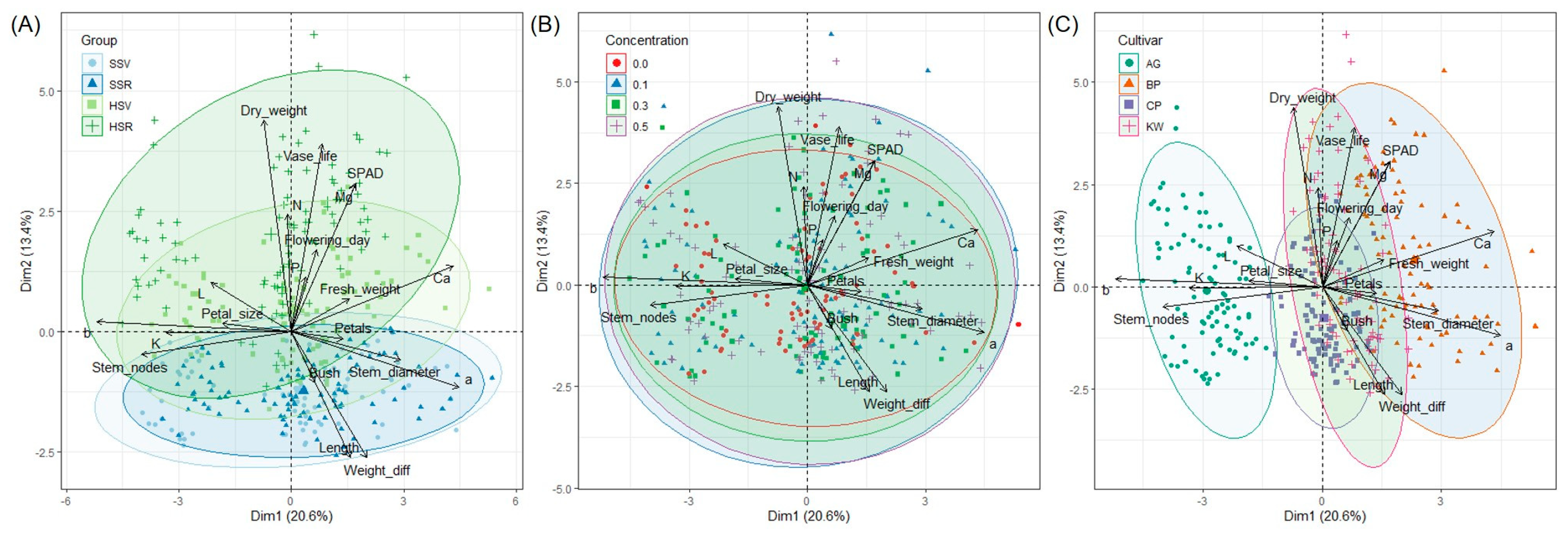
Pairwise correlations between the chemical components (N, P, K, Ca, and Mg) and vase life appeared to depend on the cultivar (Figure S11). N showed a positive correlation with vase life (r = 0.091) except for CP; P showed a positive moderate correlation with vase life for CP (r = 0.504); Mg and Ca also showed positive correlations with vase life (r = 0.259, 0.218). Only K showed a negative correlation with vase life (r = −0.219). The results of leaf analysis for all chemical components are described in the Supplementary Data (Figures S11–S16).

Most characteristics differed based on cultivars except for P content and dry weight, as summarized in Table 1. The within-cultivar variation in dry weight was relatively high compared with the between-cultivar variation of dry weight (p = 0.736). The average vase lives of BP and KW were longer than those in AG and CP (p < 0.001).

Two-way ANOVA showed that SA treatments applied with different cultivation methods and SA concentrations affected most vegetative characteristics, reproductive characteristics, and leaf chemical components. A summary of significance according to the adjusted p-values is provided in

Table 2. Sample mean and standard deviation of each characteristic by cultivar. p-values were calculated using the Kruskal–Wallis test and adjusted to account for multiple testing. *, **, and *** implying p < 0.05, p < 0.01, and p < 0.001, respectfully.

Characteristic	AG	BP	CP	KW	p-Value
Stem diameter	3.68 (0.46)	4.40 (0.60)	4.38 (0.50)	4.33 (0.53)	<0.001 ***
Stem node	8.12 (0.87)	5.93 (0.62)	7.77 (0.76)	6.96 (0.60)	<0.001 ***
Stem length	50.65 (6.17)	53.25 (7.21)	56.15 (6.66)	56.81 (8.06)	<0.001 ***
Stem bush	3.80 (1.22)	4.20 (1.25)	3.78 (0.96)	3.57 (0.89)	0.007 **
Flowering day	63.14 (5.64)	64.81 (6.11)	62.96 (4.19)	65.59 (5.26)	0.002 **
SPAD	99.97 (17.43)	118.16 (18.26)	97.86 (17.27)	121.80 (21.42)	<0.001 ***
Nitrogen	1.03 (0.28)	1.07 (0.17)	1.08 (0.28)	1.19 (0.39)	0.003 **
Phosphorus	0.75 (0.62)	0.72 (0.52)	0.81 (0.63)	0.83 (0.66)	0.212
Potassium	3.06 (0.32)	2.52 (0.20)	2.63 (0.19)	2.17 (0.26)	<0.001 ***
Calcium	0.16 (0.02)	0.34 (0.05)	0.23 (0.03)	0.22 (0.04)	<0.001 ***
Magnesium	0.50 (0.10)	0.72 (0.17)	0.50 (0.08)	0.45 (0.08)	<0.001 ***
Fresh weight	2.39 (0.44)	2.62 (0.66)	3.19 (0.56)	3.62 (0.66)	<0.001 ***
Dry weight	0.97 (0.54)	0.87 (0.39)	1.01 (0.47)	1.16 (0.86)	0.691
Weight difference	1.43 (0.48)	1.75 (0.59)	2.17 (0.57)	2.47 (1.04)	<0.001 ***
Petal number	10.73 (1.22)	11.35 (2.20)	12.27 (1.93)	12.35 (2.35)	<0.001 ***
Petal size	49.19 (5.46)	45.22 (3.37)	53.59 (4.55)	45.28 (4.21)	<0.001 ***

AG, Arena Green; BP, Blue Picote; CP, Corelli Pink; KW, Kroma White; SPAD, soil plant analysis development.

.

Table 3. Characteristics related to vase life for each cultivar.

Characteristic	AG	BP	CP	KW
Stem diameter	−	−	−	+
Stem node	−	+	+	+
Stem length	−	−	−	− **
Stem bush	−	−	+	+ *
Flowering day	+ *	+ *	+	+
SPAD	−	+ ***	+ *	+
Nitrogen	+	+	−	+
Phosphorus	+	+ *	+ ***	+
Potassium	−	−	+	− **
Calcium	+	+	+	−
Magnesium	+	+ ***	+ ***	−
Fresh weight	+ ***	+	+	+
Dry weight	+ **	+ ***	+ ***	+ ***
Weight difference	−	−	−	− ***
Petal number	+ *	−	+	+
Petal size	+	+ ***	+	+

AG, Arena Green; BP, Blue Picote; CP, Corelli Pink; KW, Kroma White; SPAD, soil plant analysis development. The sign (+ or −) indicates the direction of relationship. Significance is indicated by * (p < 0.05), ** (p < 0.01), and *** (p < 0.001). Significance has been adjusted for multiple tests.

shows the key characteristics associated with vase life, and is summarized by the direction of association (“+” implying a positive relationship and “−” implying a negative relationship) and significance (*, **, and *** implying p < 0.05, p < 0.01, and p < 0.001, respectfully, after adjusting the p-values for the multiple tests). Dry weight seemed to show a definite significant positive relationship with vase life in all cultivars. Additionally, flowering day showed a positive relationship with vase life and was significant for the AG and BP cultivars. SPAD, phosphorus, and magnesium showed positive relationships with vase life and were significant for BP and CP.

3.5. PCA

The vase life of the H cultivation group was significantly longer than that of the S cultivation group (Figure 4). Notably, the HSR group demonstrated the most suitable cultivation method for promoting vase life, whereas the S cultivation group demonstrated the most suitable cultivation method for promoting stem-related characteristics rather than vase life (Figure 4A). This study has shown that the hypothesis that increased stem diameter or stem length leads to longer vase life is incorrect. Contrary to the results of previous studies, neither stem diameter nor stem length correlated positively with vase life. Additionally, S cultivation showed a limitation whereby increases in weight difference resulted in decreased biomass. This low biomass indicates that the nutrient supply is limited in cut flowers, which can lead to a shorter vase life. In the case of SA concentration, the centroids of the variances were mostly consistent, demonstrating little average change relative to the variance (Figure 4B). However, compared with that of the control, higher SA concentrations were associated with increased vase life. The ellipses of all concentrations moved toward quadrant I, that is, toward vase life and its related characteristics. Considering the distribution of the values of various characteristics, including vase life, 0.5 mM SA was found to be the most appropriate concentration for improving vase life. Vase life was longer for the BP and KW cultivars and shorter for the AG cultivar. The BP and KW cultivars showed higher N, P, and Mg contents than those of the AG and CP cultivars, and these variables may be related to photosynthesis (Figure 4C).

PCA revealed that the characteristics most strongly correlated with vase life were dry weight, SPAD, Mg content, flowering day, and N content. We observed a strong negative correlation between weight difference and vase life, indicating that they tend to move in opposite directions. Similar to vase life, dry weight exhibited higher values in both the BP and KW cultivars. Furthermore, other characteristics exhibiting a strong correlation with vase life showed a similar trend to dry weight. The BP cultivar not only exhibited a high vase life, but also demonstrated higher fresh weight compared to other cultivars.

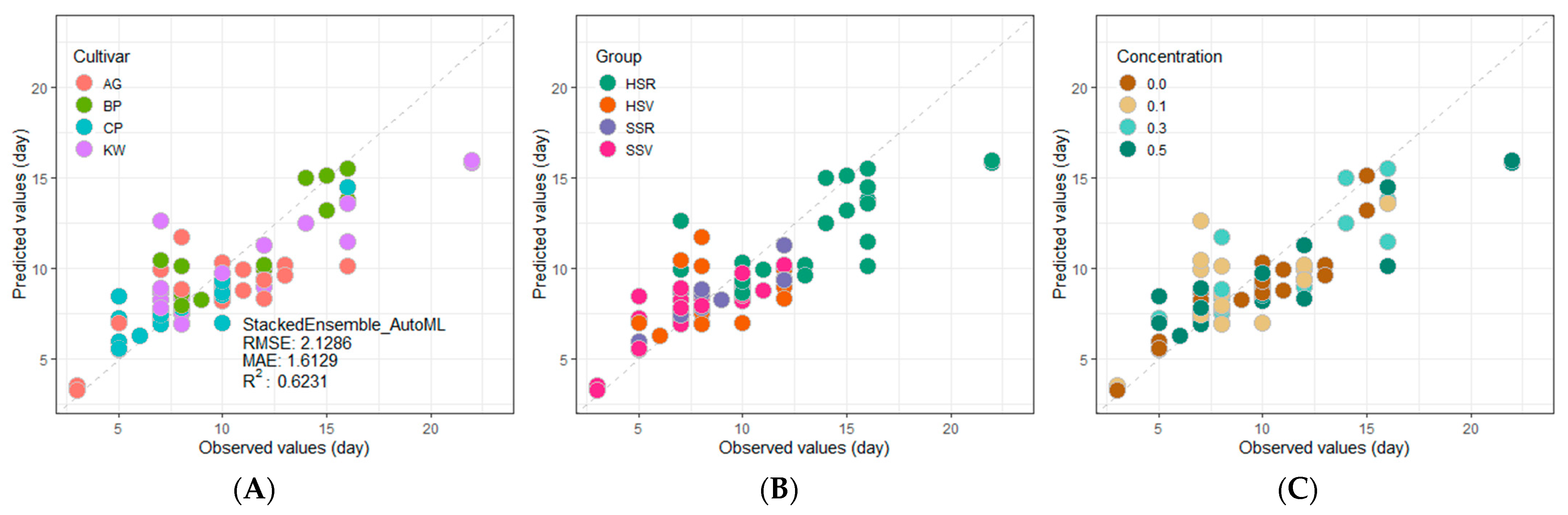
3.6. Regression Model for Predicting Vase Life Based on Biomass-Related Characteristics

Using the h2o package (https://docs.h2o.ai (accessed on 10 July 2024), v3.42.0.2), we constructed an ML model to predict vase life based on biomass-related characteristics that are positively correlated with vase life (Figure 5). This study used data from 383 samples, of which 307 samples were used to construct the training dataset and 76 samples were used to construct the test dataset (8:2 ratio). The top model selected by AutoML was a stacked ensemble model composed of a gradient boosting machine, distributed random forest, a generalized linear model, and a deep learning-based model. As shown in Figure 5, the top model resulted in an RMSE of 2.12, an MAE of 1.61, and an R² value of 0.62. Individuals predicted to have a vase life of 14 days or longer were relatively more prevalent in BP and KW compared to AG and CP. Amongst the treatment groups, individuals in the HSR group were expected to have the longest vase life. Therefore, lisianthus cultivated hydrophonically and treated with SA during the reproductive stage exhibit a prolonged vase life. As SA concentration increased, vase life also tended to lengthen. Similar to the PCA results, a vase life of the greatest duration was anticipated when the plant was treated with 0.5 mM SA.

4. Discussion

As shown in the above results, we investigated whether several characteristics during the preharvest stage were correlated with vase life and were statistically significant. Vase life correlated highly with dry weight, SPAD, flowering day, and P and Mg content. As these characteristics directly or indirectly relate to photosynthesis, this result implies that increased photosynthetic efficiency significantly relates to improved vase life. Photosynthesis is the primary process responsible for biomass production, which ultimately contributes to dry weight accumulation. High dry weight indicates sufficient vegetative growth and carbohydrate accumulation. Therefore, we can infer that a longer vegetative period allowing for sufficient photosynthesis (indicated by a later flowering day), a higher SPAD value reflecting efficient leaf photosynthesis, and increased Mg content—a key component of chlorophyll—contribute to an extended vase life. This suggests that higher photosynthetic efficiency, reflected in greater dry weight, positively influences vase life. The increase in dry weight serves as a source of carbohydrates that determine the longevity of cut flowers after flower cutting. Furthermore, we propose that high tissue water content also contributes to prolonged vase life. It appears that the BP cultivar’s longer vase life is attributable to a combination of high carbohydrate content generated through photosynthesis and high tissue water content, both exceeding those observed in other cultivars. While AG exhibits a shorter vase life, it stands out due to its comparatively larger petal size compared to other cultivars. The consumption of carbohydrates for the development and maintenance of large leaves, coupled with water loss due to respiration and transpiration in these larger leaves, contributes to a shorter vase life in AG.

Among the leaf chemical components, Ca content was higher in the BP cultivar and may be closely related to the purple color of the BP cultivar. Flower color is determined by the anthocyanin flavonoid concentration [34,35] and levels of other colorless or pale-yellow flavonols known as copigments [36]. The copigmentation phenomenon is defined as copigment-mediated anthocyanin color intensification [37]. Among the various lisianthus color pigments, the blue pigment is a metal complex of anthocyanin and flavone glycoside with one ferric, one magnesium, and two calcium ions [38]. The high levels of Mg and Ca in the BP cultivar, which is characterized by purple coloration, may be attributed to this association.

This ML model was developed to estimate vase life, a postharvest characteristic, based on pre-harvest biomass-related characteristics. Initially, the model was developed incorporating all investigated traits: vegetative and reproductive characteristics, as well as leaf chemical components, as variables for predicting vase life. Furthermore, since samples with vase life shorter than 10 days or exceeding 12 days were considered to potentially lower the R² value, these outliers were removed, and model development was attempted again. However, all attempts resulted in a further decrease in the R² value. Therefore, based on the information gleaned from statistical analysis, we proceeded to exclude variables exhibiting a negative correlation with vase life from the feature set. Dry weight, which demonstrated the highest correlation with vase life, was also selected as a key feature in the stacked ensemble model, the top-performing model identified by AutoML. Following dry weight, SPAD value, Mg content and flowering day emerged as the next most significant features. In conclusion, features with a negative correlation did not contribute to improving model performance in the machine learning model predicting vase life. The characteristics that exhibit a negative correlation with vase life, such as weight difference, were excluded as features in this model. Only characteristics with a positive correlation with vase life were included in the model development. The analysis included the following features: flowering day and SPAD from vegetative characteristics; fresh weight, dry weight, petal number, and petal size from reproductive characteristics; and all leaf chemical components except for potassium. These characteristics were identified as the most influential variables in explaining vase life within our machine learning model, suggesting their potential for use in developing a predictive model of vase life.

Additional feature engineering techniques were also explored. Since dry weight exhibited a rightward skew, we attempted to transform the data to a normal distribution using logarithmic values, but this did not yield the desired outcome for analysis. While we aimed to construct a dataset as close to normal distribution as possible by excluding outliers, this resulted in a smaller sample size, presenting a new challenge. Therefore, we realized that increasing the sample size and refining the data through further feature engineering will be crucial for future analysis. Applying these approaches is anticipated to lead to the development of a more precise prediction model.

Choi and Lee [39] constructed a logistic regression model to estimate the vase life of cut roses utilizing thermal image data. While this model achieved 100% accuracy, it was trained only on data from a single cultivar, and therefore, the application of this model to other cultivars has been reported to result in errors. According to In et al. [40], a vase life prediction model was developed utilizing various environmental and phenotypic parameters. The models, developed through multiple regression analysis, reported R² values ranging from 0.60 to 0.62. Kim et al. [41] developed the deep learning model, YOLOv5, for predicting the vase life of cut roses from hyperspectral image data. The model demonstrated a high predictive accuracy, with R² values ranging from 0.83 to 0.86 across different cultivars. Our previous study focused on developing a vase life prediction model based on petal colorimetric data and SPAD values for cut flowers [10]. The ML model based on colorimetric data exhibited a high predictive performance with an R² of 0.95, while the model utilizing SPAD values demonstrated a performance with an R² of 0.69. This model demonstrated a high predictive performance because the direct correlation between petal color changes and vase life was expected. The studies by Choi and Lee [39] and Kim et al. [41] were based on image data from thermal or hyperspectral cameras, while the study by In et al. [40] and our study have in common that they are based on phenotypic data of cut flowers. There are not many studies that estimate vase life based on the phenotype of the preharvest stage of a cut flower. In addition, it was observed that models relying on phenotypes not directly correlated with vase life exhibited lower predictive performance. Our ML model demonstrated a comparable predictive performance to the model developed by In et al. [40]. This study aimed to investigate the relationship between characteristics measurable during the pre-harvest stage and vase life, a key indicator of cut flower quality, with the goal of developing methods for predicting vase life. This study’s phenotype-based model does not just illustrate the relationship between traits and vase life; it allows for the establishment of cultivar-specific environmental and management conditions that can enhance vase life.

As mentioned earlier, the HSR group showed a much longer vase life than those of the other treatment groups; therefore, the HSR group showed the highest variable importance in the ML model. Additionally, the model showed a trend towards longer vase life as the SA concentration increased to 0.5 mM. Among the four cultivars, BP and KW exhibited the longest vase lives. These results suggest that floriculturists should cultivate the BP and KW cultivars in an HSR environment and apply the 0.5 mM SA treatment to ensure a long vase life. The HSR environment and SA application (0.5 mM) resulted in longer vase life, implying that this environment and management elicits an enhancement effect on photosynthetic efficiency in the BP and KW cultivars compared with that of the other cultivation environments and management conditions. By optimizing growing environments and implementing effective agricultural management practices that promote these traits, growers can potentially enhance vase life in lisianthus cultivars. By elucidating the conditions that maximize the interaction between genotype (cultivar), environment, and management, we anticipate being able to optimize vase life for each specific cultivar. This will be a focus of our future research endeavors. This predictive model, which can estimate vase life based on pre-harvest characteristics, is poised to significantly impact the standardization of cut flower quality assessments. Given the large volume of international importation and exportation of cut lisianthus flowers, future studies are needed to better understand cultivar-specific factors and accurately predict the vase life of cut flowers so as to benefit floriculture workers and consumers.

5. Conclusions

Biomass refers to the total quantity of organic matter produced by plants via photosynthesis. Although increased biomass may not be the only factor contributing to prolonged vase life, the hypothesis that increased biomass promotes abundant nutrients and longevity is scientifically valid. In this study, we observed changes in biomass-related traits and relationships between increased biomass and prolonged vase life in four lisianthus cultivars. The cultivation method and SA treatment timing and concentration affected most biomass-related traits in all four cultivars, and some traits showed significant positive associations with prolonged vase life. A commonly observed trend across the four cultivars was that dry weight showed significant association with vase life. Furthermore, dry weight was the strongest predictor of vase life according to the AutoML model. Finally, these findings indicate that floriculturists could achieve prolonged vase life by cultivating the BP and KW cultivars in an HSR environment and applying 0.5 mM SA treatment.

References

1. Ohkawa, K.; Sasaki, E. Eustoma (Lisianthus)—Its past, present, and future. In International Symposium on Cut Flowers in the Tropics, ISHS Acta Horticulturae, Bogota; Fischer, G., Angarita, A., Eds.; ISHS: Brussels, Belgium, 1999; pp. 423–428. Available online: https://www.actahort.org/books/482/482_61.htm (accessed on 1 July 2024).
2. Ichimura, K. Improvement of postharvest life in several cut flowers by the addition of sucrose. Jpn. Agricult. Res. Quart. 1998, 32, 275–280. [Google Scholar]
3. Lakshmaiah, K.; Ganga, M.; Subramanian, S.; Santhi, R. Role of post-harvest treatments in improving vase life of lisianthus (Eustoma grandiflorum) variety Mariachi Blue. Int. J. Chem. Stud. 2019, 7, 247–249. [Google Scholar]
4. Shimizu-Yumoto, H.; Ichimura, K. Postharvest physiology and technology of cut Eustoma flowers. Jpn. Soc. Hort. Sci. 2010, 79, 227–238. [Google Scholar] [CrossRef]
5. Skutnik, E.; Łukaszewska, A.; Rabiza-Świder, J. Effects of postharvest treatments with nanosilver on senescence of cut lisianthus (Eustoma grandiflorum (Raf.) Shinn.) flowers. Agronomy 2021, 11, 215. [Google Scholar] [CrossRef]
6. Bahrami, S.N.; Zakiwadeh, H.; Hamidoghli, Y. Salicylic acid retards petal senescence in cut lisianthus (Eustoma grandiflorum ‘Miarichi Grand White’) flowers. Hortic. Environ. Biotechnol. 2013, 54, 519–523. [Google Scholar] [CrossRef]
7. Islam, N.; Patil, G.G.; Gislerød, H.R. Effects of pre- and postharvest conditions on vase life of Eustoma grandiflorum (Raf.) Shinn. Europ. J. Hort. Sci. 2003, 68, 272–278. [Google Scholar]
8. Kamiab, F.; Fahreji, S.S.; Bahramabadi, E.Z. Antimicrobial and physiological effects of silver and silicon nanoparticles on vase life of lisianthus (Eustoma grandiflora cv. Echo) flowers. Int. J. Hortic. Sci. Technol. 2017, 4, 135–144. [Google Scholar]
9. Liao, L.J.; Lin, Y.H.; Huang, K.L.; Chen, W.S. Vase life of Eustoma grandiflorum as affected by aluminum sulfate. Bot. Bull. Acad. Sinica 2001, 42, 35–38. [Google Scholar]
10. Kwon, H.S.; Leporini, C.; Kim, S.; Heo, S. Prolonged vase life by salicylic acid treatment and prediction of vase life using petal color senescence of cut lisianthus. Postharvest Biol. Technol. 2024, 209, 112726. [Google Scholar] [CrossRef]
11. Proietti, S.; Scariot, V.; De Pascale, S.; Paradiso, R. Flowering mechanisms and environmental stimuli for flower transition: Bases for production scheduling in greenhouse floriculture. Plants 2022, 11, 432. [Google Scholar] [CrossRef] [PubMed]
12. Xu, N.; Meng, L.; Tang, F.; Du, S.; Xu, Y.; Kuang, S.; Zhang, Y. Plant spacing effects on stem development and secondary growth in Nicotiana tabacum. Agronomy 2023, 13, 2142. [Google Scholar] [CrossRef]
13. Naghshi Band Hasani, R.; Yousefi, S.; Zare Hagi, D. The effect of cut stem length treatment on vase life and water relations of roses (Rosa hybrida) cv. ‘Bingo White’. J. Ornam. Plants 2020, 10, 109–119. [Google Scholar]
14. López-Guerrero, A.G.; Rodriguez-Hernandez, A.M.; Mounzer, O.; Zenteno-Savin, T.; Rivera-Cabrera, F.; Izquierdo-Oviedo, H.; Soriano-Melgar, L.D.A.A. Effect of oligosaccharins on the vase life of lisianthus (Eustoma grandiflorum Raf.) cv. ‘Mariachi blue’. J. Hortic. Sci. Biotechnol. 2020, 95, 316–324. [Google Scholar] [CrossRef]
15. Janowska, B.; Andrzejak, R. Plant growth regulators for the cultivation and vase life of geophyte flowers and leaves. Agriculture 2023, 13, 855. [Google Scholar] [CrossRef]
16. Piri, M.; Jabbarzadeh, Z. The effect of foliar application of salicylic acid, spermidine and sodium nitroprusside on some growth and flowering characteristics, photosynthetic pigments and vase life of lisianthus ‘Mariachi Blue’. J. Hortic. Sci. 2023, 36, 917–936. [Google Scholar]
17. Canet, J.V.; Dobón, A.; Ibáñez, F.; Perales, L.; Tornero, P. Resistance and biomass in Arabidopsis: A new model for salicylic acid perception. Plant Biotechnol. J. 2010, 8, 126–141. [Google Scholar] [CrossRef]
18. Gorni, P.H.; Pacheco, A.C.; Moro, A.L.; Silva, J.F.A.; Moreli, R.R.; Miranda, G.R.; Silva, R.M.G. Salicylic acid foliar application increases biomass, nutrient assimilation, primary metabolites and essential oil content in Achillea millefolium L. Sci. Hortic. 2020, 270, e109436. [Google Scholar] [CrossRef]
19. Ibrahim, M.; Omar, H.; Mohd Zain, N. Salicylic acid enhanced photosynthesis, secondary metabolites, antioxidant and lipoxygenase inhibitory activity (LOX) in Centella asiatica. Annu. Res. Rev. Biol. 2017, 17, 1–14. [Google Scholar] [CrossRef]
20. Acero, L.H.; Tuy, F.S.; Virgino, J.S. Potassium aluminum sulfate solution on the vase life of sampaguita (Jasminum sambac) flowers. J. Med. Bioeng. 2016, 5, 33–36. [Google Scholar] [CrossRef]
21. Jowkar, M.M.; Khalighi, A.; Kafi, M.; Hassanzadeh, N. Evaluation of aluminum sulfate as vase solution biocide on postharvest microbial and physiological properties of ‘Cherry Brandy’ rose. Acta Hortic. 2013, 1012, 615–626. [Google Scholar] [CrossRef]
22. Kazemi, M. Effect of cobalt, silicon, acetylsalicylic acid and sucrose as novel agents to improve vase-life of Argyranthemum flowers. Trends Appl. Sci. Res. 2012, 7, 579–583. [Google Scholar] [CrossRef]
23. Singh, A.K.; Sisodia, A.; Pal, A.K.; Barman, K. Effect of sucrose and aluminium sulphate on postharvest life of lilium cv. Monarch. J. Hill Agric. 2016, 7, 204–208. [Google Scholar] [CrossRef]
24. Subbaramamma, P.; Bhaskar, V.V. Role of beneficial elements in post-harvest vase life of cut flowers. Pharma Innov. 2023, 12, 1242–1250. [Google Scholar]
25. Mendoza-Villarreal, R.; Valdez-Aguilar, L.A.; Sandoval-Rangel, A.; Robledo-Torres, V.; Benavides-Mendoza, A. Tolerance of lisianthus to high ammonium levels in rockwool culture. J. Plant Nutr. 2015, 38, 73–82. [Google Scholar] [CrossRef]
26. Halevy, A.H.; Mayak, S. Senescence and postharvest physiology of cut flowers—Part 2. In Horticultural Reviews; John Wiley & Sons: New York, NY, USA, 1981; Volume 3, pp. 59–143. [Google Scholar]
27. Takeno, K. Stress-induced flowering: The third category of flowering response. J. Exp. Bot. 2016, 67, 4925–4934. [Google Scholar] [CrossRef]
28. Bradstreet, R.B. Kjeldahl method for organic nitrogen. Anal. Chem. 1954, 26, 185–187. [Google Scholar] [CrossRef]
29. Cavell, A.J. The colorimetric determination of phosphorus in plant materials. J. Sci. Food Agric. 1955, 6, 479–480. [Google Scholar] [CrossRef]
30. Benjamini, Y.; Yekutieli, D. The control of the false discovery rate in multiple testing under dependency. Ann. Stat. 2001, 29, 1165–1188. [Google Scholar] [CrossRef]
31. Fryda, T.; LeDell, E.; Gill, N.; Aiello, S.; Fu, A.; Candel, A.; Click, C.; Kraljevic, T.; Nykodym, T.; Aboyoun, P.; et al. H2O: R Interface for the ‘H2O’ Scalable Machine Learning Platform; R Package Version 3.40.0.4.; R Core Team: Vienna, Austria, 2023; Available online: https://docs.h2o.ai/h2o/latest-stable/h2o-r/docs/articles/getting_started.html (accessed on 10 July 2024).
32. Lares, B. Lares: Analytics & Machine Learning Sidekick; R Package Version 5.2.2; R Core Team: Vienna, Austria, 2023; Available online: https://laresbernardo.github.io/lares/ (accessed on 10 July 2024).
33. Zhang, R.; Yang, P.; Liu, S.; Wang, C.; Liu, J. Evaluation of the methods for estimating leaf chlorophyll content with SPAD chlorophyll meters. Remote Sens. 2022, 14, 5144. [Google Scholar] [CrossRef]
34. Almeida, J.M.D.; Calaboni, C.; Rodrigues, P.H.V. Pigments in flower stems of lisianthus under different photoselective shade nets. Ornam. Hortic. 2021, 27, 535–543. [Google Scholar] [CrossRef]
35. Gao, L.; Yang, H.; Liu, H.; Yang, J.; Hu, Y. Extensive transcriptome changes underlying the flower color intensity variation in Paeonia ostii. Front. Plant Sci. 2016, 6, 1205. [Google Scholar] [CrossRef] [PubMed]
36. Iwashina, T. Contribution to flower colors of flavonoids including anthocyanins: A review. Nat. Prod. Commun. 2015, 10, 529–544. [Google Scholar] [CrossRef] [PubMed]
37. Trouillas, P.; Sancho-García, J.C.; De Freitas, V.; Gierschner, J.; Otyepka, M.; Dangles, O. Stabilizing and modulating color by copigmentation: Insights from theory and experiment. Chem. Rev. 2016, 116, 4937–4982. [Google Scholar] [CrossRef]
38. Takeda, K. Blue metal complex pigments involved in blue flower color. Proc. Jpn. Acad. Ser. B. Phys. Biol. Sci. 2006, 82, 142–154. [Google Scholar] [CrossRef]
39. Choi, S.Y.; Lee, A.K. Development of a cut rose longevity prediction model using thermography and machine learning. Hortic. Sci. Technol. 2020, 31, 675–685. [Google Scholar] [CrossRef]
40. In, B.C.; Inamoto, K.; Doi, M.; Park, S.A. Using thermography to estimate leaf transpiration rates in cut roses for the development of vase life prediction models. Hortic. Environ. Biotechnol. 2016, 57, 53–60. [Google Scholar] [CrossRef]
41. Kim, Y.T.; Ha, S.T.T.; In, B.C. Development of a longevity prediction model for cut roses using hyperspectral imaging and a convolutional neural network. Front. Plant Sci. 2024, 14, 1296473. [Google Scholar] [CrossRef] [PubMed]
Figure 1. Effects of treatment groups according to cultivar on SPAD data (A), the effect of salicylic acid (SA) concentration according to the treatment group (B), and the effect of SA concentration according to the cultivar (C).
Agriculture 14 01543 g001
Figure 2. Correlation matrix plot between correlation coefficients and corresponding significance levels between reproductive characteristics and vase life. The diagonal boxes show the variable distributions split by cultivars. The lower boxes are composed of scatter plots, and the upper boxes show the Pearson correlation coefficients with significance level (as asterisks) by cultivars. Each significance level is associated with a symbol: p-value 0.001 (***), 0.01 (**), 0.05 (*), and not significant (no asterisk). AG, Arena Green; BP, Blue Picote; CP, Corelli Pink; KW, Kroma White.
Agriculture 14 01543 g002
Figure 3. Effect of treatment groups according to the cultivar on the dry weight (A), effect of salicylic acid (SA) concentration according to the treatment group (B), and effect of SA concentration according to the cultivar (C).
Agriculture 14 01543 g003
Figure 4. Principal component analysis (PCA) biplots showing the PCA scores of the explanatory variables as vectors (black arrows) and individuals (each point). (A) Each class represents SSV (sky blue circles), SSR (blue triangles), HSV (pale green squares), and HSR (green crosses). (B) Each class represents salicylic acid concentration at 0.0 (red circles), 0.1 (blue triangles), 0.3 (green squares), and 0.5 mM (violet crosses). (C) Each class represents a lisianthus cultivar: AG (green circles), BP (red triangles), CP (violet squares), and KW (purple crosses).
Agriculture 14 01543 g004
Figure 5. Regression plot for estimating vase life of cut lisianthus flowers based on biomass-related characteristics using AutoML according to cultivar (A), treatment group (B), and SA concentration (C). The horizontal axis in the scatter plot represents the field-observed vase life, whereas the vertical axis represents the vase life predicted by the model. The 1:1 slope is shown as a gray dotted line.
Agriculture 14 01543 g005