Intelligent Surface Recognition for Autonomous Tractors Using Ensemble Learning with BNO055 IMU Sensor Data

Abstract

This study aims to enhance the navigation capabilities of autonomous tractors by predicting the surface type they are traversing using data collected from BNO055 Inertial Measurement Units (IMU sensors). IMU sensor data were collected from a small mobile robot driven over seven different floor surfaces within a university environment, including tile, carpet, grass, gravel, asphalt, concrete, and sand. Several machine learning models, including Logistic Regression, K-Neighbors, SVC, Decision Tree, Random Forest, Gradient Boosting, AdaBoost, and XGBoost, were trained and evaluated to predict the surface type based on the sensor data. The results indicate that Random Forest and XGBoost achieved the highest accuracy, with scores of 98.5% and 98.7% in K-Fold Cross-Validation, respectively, and 98.8% and 98.6% in an 80/20 Random State split. These findings demonstrate that ensemble methods are highly effective for this classification task. Accurately identifying surface types can prevent operational errors and improve the overall efficiency of autonomous systems. Integrating these models into autonomous tractor systems can significantly enhance adaptability and reliability across various terrains, ensuring safer and more efficient operations.

1. Introduction

Autonomous tractors, designed to perform a range of agricultural tasks intelligently—such as tillage, sowing, crop protection, and fertilization—require accurate environmental perception to ensure safe and efficient navigation [1,2]. The problem at hand is the difficulty these vehicles face in identifying and adapting to different surface types, which can lead to operational inefficiencies and safety hazards [3]. Proper surface recognition is crucial for safe and efficient navigation [4,5].

Previous research has explored the use of Inertial Measurement Units (IMUs) and other sensor technologies for surface recognition in robotics [6,7,8,9,10,11,12]. Several studies have employed machine learning techniques to classify surface types based on sensor data. A comprehensive review discusses various machine learning (ML) applications in precision agriculture, including crop monitoring, yield prediction, and soil health assessment, highlighting the importance of ML techniques in enhancing agricultural efficiency and sustainability [13]. This is analogous to improving the operational efficiency of autonomous tractors through accurate terrain recognition models. Evaluating the performance of the Sentinel-2 satellite for mapping submerged aquatic vegetation (SAV) using different algorithms emphasizes the importance of selecting and comparing various ML methods to improve detection accuracy, similar to the approach of evaluating multiple ML models for surface type prediction [14]. A deep learning method for segmenting agricultural fields using convolutional neural networks (CNNs) on multi-temporal satellite imagery demonstrates high accuracy and robustness, paralleling the goal of using advanced models, like Random Forest and XGBoost, to achieve accurate and robust surface-type predictions for autonomous tractors [15]. Integrating satellite imagery with ML models to enhance crop yield prediction showcases the utility of combining ML techniques for improved agricultural decision making, similar to integrating IMU sensor data with ensemble learning techniques for better terrain adaptation in autonomous tractors [16]. Additionally, advancements in precision irrigation and water use efficiency, highlighted through innovative technologies, like sensor-based systems and data analytics, reflect the broader theme of leveraging advanced ML models in order to enhance the safety and optimize the performance of self-driving agricultural equipment [16,17].

The primary research gap addressed by this study is the application of BNO055 IMU sensor data for real-time terrain recognition in autonomous tractors. While the existing literature explores various ML applications in agriculture, it lacks a focus on integrating IMU sensors with ensemble learning techniques to improve autonomous vehicle performance across diverse terrains. This research contributes to bridging this gap by developing and evaluating ML models specifically for surface type prediction, enhancing the adaptability, efficiency, and safety of autonomous agricultural machinery. This study advances the state of the art by applying ensemble learning methods, particularly Random Forest and XGBoost, to BNO055 IMU sensor data, demonstrating improved accuracy over traditional models. Practically, it offers a robust framework for real-time terrain adaptation in autonomous tractors, which is crucial for optimizing navigation capabilities and operational efficiency in varied agricultural environments.

To achieve this, this study utilized a rich dataset collected from the BNO055 sensor, whose acceleration, gyroscope, and magnetometer readings are essential for capturing the nuanced differences between various environment surfaces. Several machine learning models, including Logistic Regression, K-Neighbors, SVC, Decision Tree, Random Forest, Gradient Boosting, AdaBoost, and XGBoost, were chosen for evaluation due to their distinct strengths in handling different types of data and classification problems. Logistic Regression offers simplicity and interpretability, making it a good baseline model [18]. K-Neighbors is effective for capturing local data patterns [19]. SVC is known for its robustness in high-dimensional spaces [20]. Decision Tree provides a clear visualization of decision-making processes [21]. Ensemble methods like Random Forest [22], Gradient Boosting [23], AdaBoost [24], and XGBoost [25] are highly effective because they leverage the advantages of several models to improve prediction accuracy and resilience. Random Forest and XGBoost exhibit their capacity to effectively manage intricate relationships among sensor data and mitigate the issue of overfitting.

The results suggest that ensemble approaches, including Random Forest and XGBoost, are extremely efficient for predicting surface types using IMU sensor data. The remarkable precision and resilience of these models indicate that they can greatly improve the navigation capabilities of autonomous tractors, guaranteeing consistent performance on different types of terrain. Ultimately, this study showcases the capacity of employing sophisticated machine learning algorithms to enhance surface identification in self-driving tractors. This study makes a valuable contribution to the advancement of autonomous agricultural systems by overcoming the shortcomings of current solutions and obtaining a high level of forecast accuracy. Building on these findings, this research specifically focuses on enhancing the navigation capabilities of autonomous tractors by predicting surface types using data collected from BNO055. This study primarily examines surface types suitable for tasks like transporting goods or supplies in agricultural settings. The system improves surface recognition, enabling autonomous tractors to adapt to different terrains, particularly in regulating speed.

2. Materials and Methods

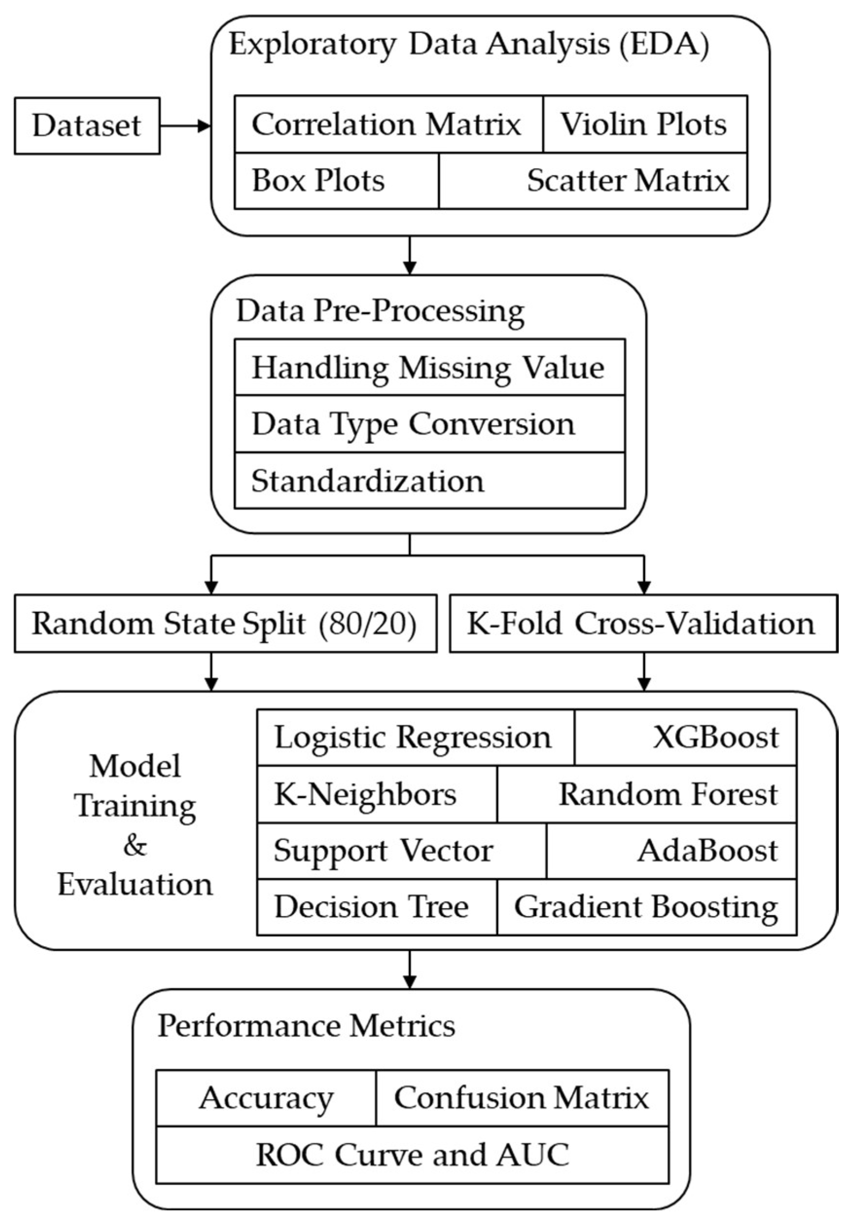
2.1. Research Overview

Figure 1 presents an outline of this study, starting with the collection of the dataset and performing Exploratory Data Analysis to comprehend the distribution and characteristics of the dataset [26]. Boxplots were generated for each feature to visualize the distribution and identify outliers. Additionally, a scatter matrix was plotted for the numeric features to examine the relationships between different sensor readings. The collected dataset underwent several preprocessing steps to ensure data quality and consistency [27]. First, missing values in the dataset were identified and handled by dropping rows with missing data. Next, columns that initially had “gyro-Y”, “gyro-Z”, “mag-X”, and “mag-Y” type objects were converted to numeric types to facilitate analysis. Finally, the characteristics were normalized using the StandardScaler function from the scikit-learn library to guarantee that they had an average of 0 and a standard deviation of 1. This phase was essential in enhancing the efficacy of machine learning algorithms.

Several machine learning models were employed to predict the surface type based on the IMU sensor data. The models included Logistic Regression 1.3.2, K-Neighbors classifier 1.3.2, Support Vector Classifier (SVC) 1.3.2, Decision Tree classifier 1.3.2, Random Forest classifier 1.3.2, Gradient Boosting classifier 1.3.2, AdaBoost classifier 1.3.2, and XGBoost classifier 2.1.1. The models were evaluated using two different approaches: Random State split (80/20) [28] and K-Fold Cross-Validation [29,30]. Random State split involved dividing the dataset into training and testing sets with an 80/20 ratio. The training set was used to train the models, while the testing set was employed to assess their performance. Accuracy scores were calculated to evaluate and compare the performance of the models.

For K-Fold Cross-Validation, a 5-fold cross-validation was conducted to ensure a robust and unbiased evaluation. The dataset was partitioned into 5 folds, with each fold serving as a testing set once, while the remaining folds were used as the training set. The reason for using 5 folds was to strike a balance between computational efficiency and reliable performance estimates, as a higher number of folds would have increased computation time without significant performance improvements. The method was iterated five times to calculate the average accuracy score for each model, providing a more comprehensive and stable measure of model performance.

The evaluation of each model was conducted using the following metrics. Accuracy refers to the ratio of accurately classified cases to the total number of instances. The confusion matrix provides a summary of the model’s performance by displaying the number of true positives, false positives, true negatives, and false negatives for each class. The ROC curve and AUC assess the model’s capability to differentiate between classes [31,32,33]. The following libraries and tools were used in this study: scikit-learn for machine learning model implementation, data preprocessing, and evaluation; pandas for data manipulation and analysis; numpy for numerical computations; matplotlib and seaborn for data visualization; Google Colab for code execution and environment setup; and xgboost for implementing the XGBoost classifier.

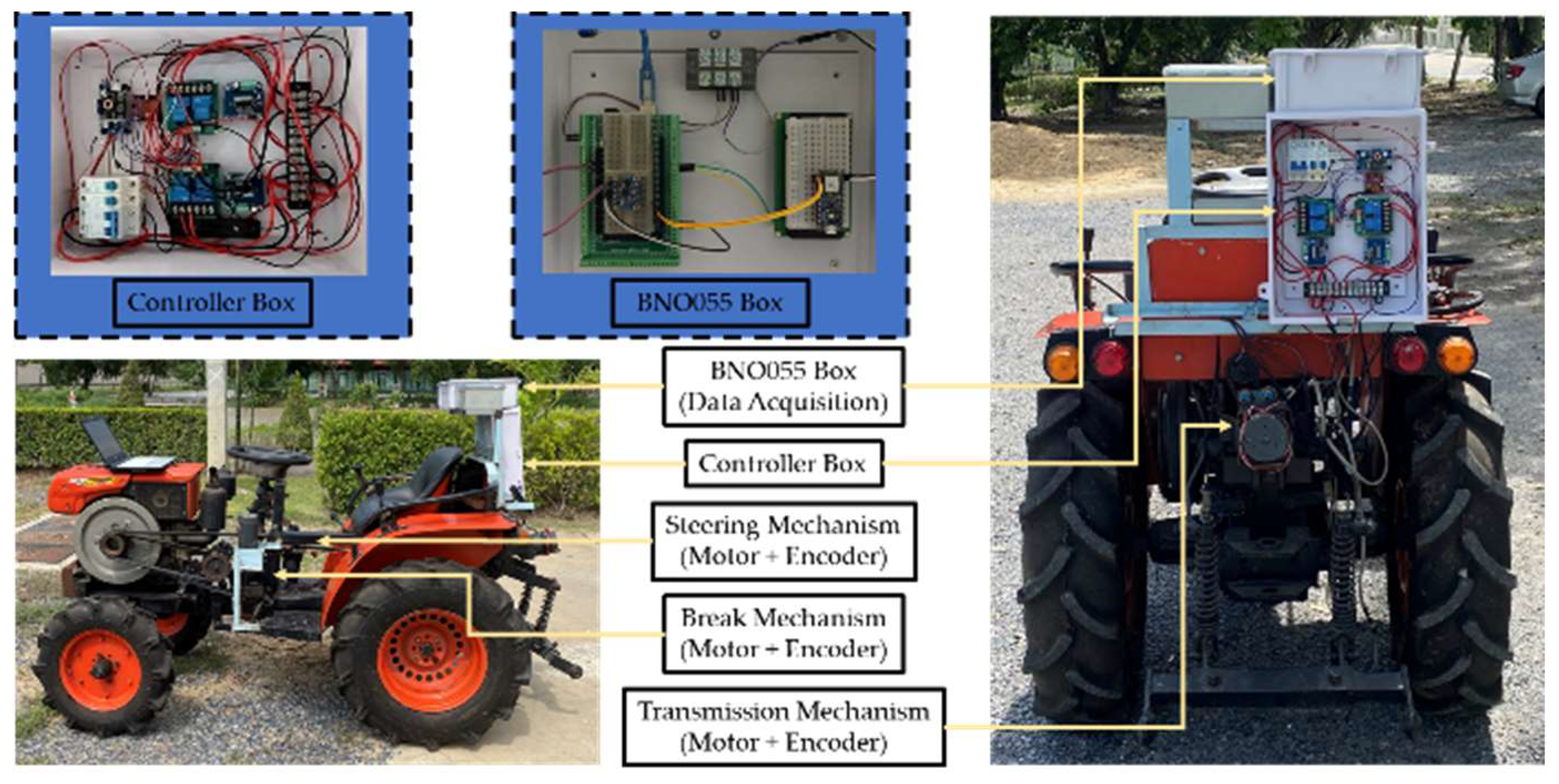
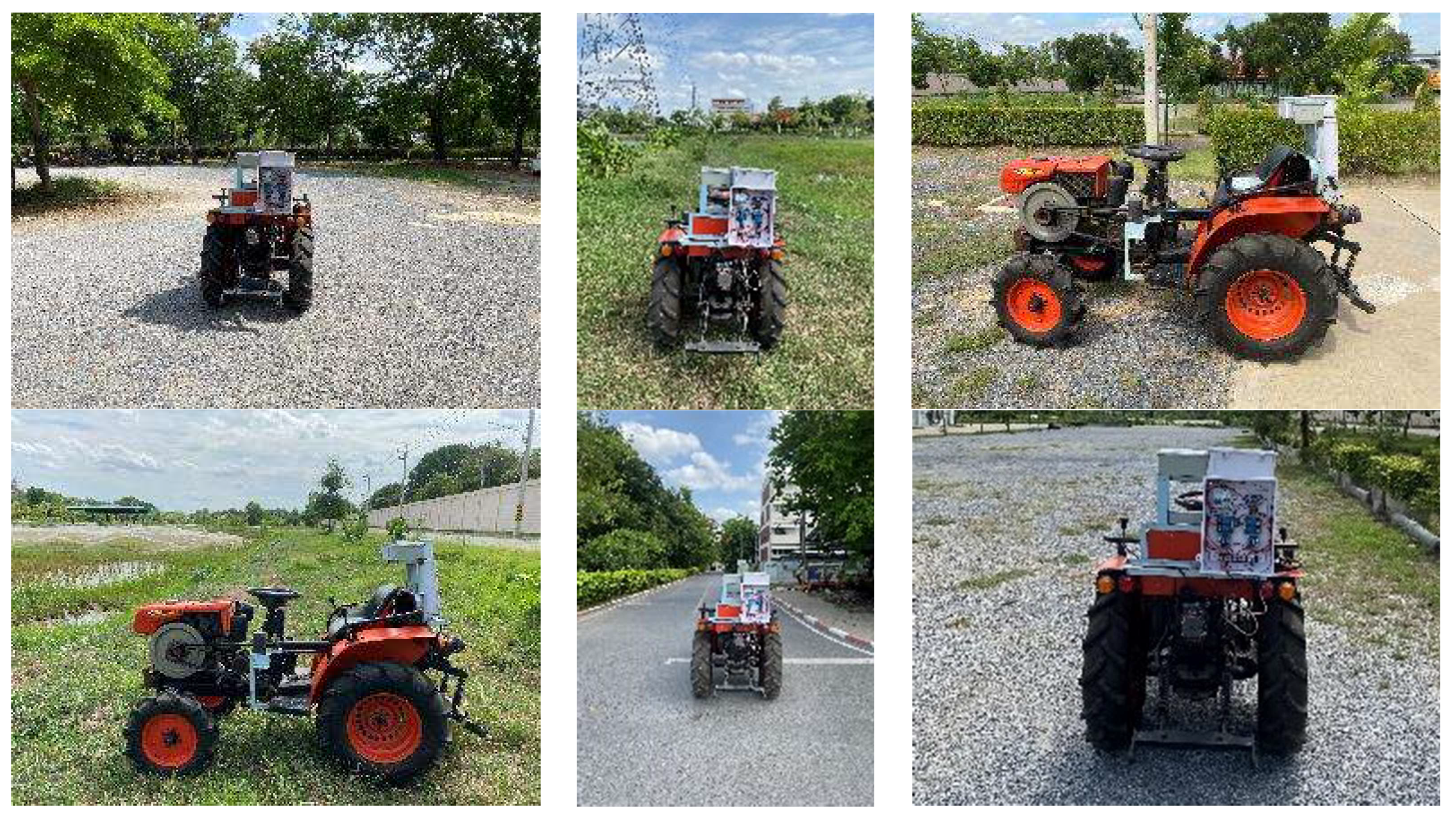
2.2. Data Collection and Field Testing

IMU sensor data were collected from a BNO055 sensor mounted on a small mobile tractor robot in Figure 2. The robot was driven over seven different floor surfaces (scenarios) within the university environment. The selection of these surfaces—such as asphalt, gravel, concrete + gravel, and soil + grass—was based on their relevance to agricultural and outdoor settings where autonomous tractors typically operate. These surface types represent a mix of hard, loose, and mixed terrains that autonomous tractors would commonly encounter in real-world agricultural tasks. The data collected encompassed acceleration, gyroscope, and magnetometer readings, providing a comprehensive dataset for analysis.

Table 1. Scenario details.

Output ID	Scenario	Track	Surface	Longitude	Latitude
0	Scenario 1	Around	Asphalt	14.134466	100.610301
1	Scenario 2	Around	Gravel	14.134458	100.609802
2	Scenario 3	Zigzag	Gravel	14.134458	100.609802
3	Scenario 4	Around	Concrete + Gravel	14.132445	100.613033
4	Scenario 5	Zigzag	Concrete + Gravel	14.132445	100.613033
5	Scenario 6	Around	Soil + Grass	14.135185	100.611764
6	Scenario 7	Zigzag	Soil + Grass	14.135185	100.611764

provides details about different scenarios represented in the image, including the scenario identifier, track type, surface type, and geographic coordinates (longitude and latitude). Each row in the table corresponds to a specific scenario, detailing its unique characteristics. The columns in the table are as follows: Output ID, Scenario, Track, Surface, Longitude, and Latitude. Output ID is a unique identifier starting from 0, while the Scenario column describes the different scenarios labeled from “Scenario 1” to “Scenario 7”. The Track column indicates the type of track used, either “Around” or “Zigzag”, and the Surface column describes the surface type, such as asphalt, gravel, concrete + gravel, and soil + grass. The Longitude and Latitude columns provide the geographic coordinates for each scenario’s location.

The research experiment (Figure 3) involves deploying a machine learning model onto embedded systems for real-time surface classification in controlling a small robot tractor. The machine learning model is first developed and trained and then saved in .joblib format. Using the microMLgen library, the model is converted into a .h file, which is uploaded to the Arduino Nano 33 BLE. This microcontroller is tasked with making predictions or classifications based on incoming sensor data from the BNO055 sensor, which is connected to an Arduino Mega. The Arduino Mega collects data such as acceleration, gyroscope, and magnetometer readings from the BNO055 sensor and sends it to the Arduino Nano 33 BLE for real-time classification. Additionally, Arduino Mega is linked to a controller box that controls a small robot tractor. Mega also connects to a laptop for data collection, allowing researchers to gather both sensor readings and classification results for further analysis. The combined system facilitates surface recognition for the robot tractor, enabling autonomous adaptation to various terrains, especially in regulating the tractor’s speed.

Figure 4 and Figure 5 show satellite and environment views of the locations for each scenario with paths marked in red and green. Scenario 1 features an “Around” track type on an asphalt surface, located at 14.134466 longitude and 100.610301 latitude (Figure 4a). Scenario 2 also has an “Around” track type but on a gravel surface, with coordinates 14.134458 and 100.609802 (Figure 4b). In Scenario 3 (Figure 4c), the track is a “Zigzag” pattern over a gravel surface, sharing the same coordinates as Scenario 2. Scenario 4 has an “Around” track type on a combination of concrete and gravel surfaces, located at 14.132445 and 100.613033 (Figure 4d). Similarly, Scenario 5 (Figure 4e) features a “Zigzag” track over concrete and gravel surfaces at the same coordinates as Scenario 4. Scenario 6 has an “Around” track type on a soil and grass surface, with coordinates 14.135185 and 100.611764 (Figure 4f). Lastly, Scenario 7 (Figure 4g) presents a “Zigzag” track over soil and grass surfaces, sharing the same coordinates as Scenario 6. These scenarios seem to be designed for testing or evaluating outdoor activities involving movement over different surfaces and paths. The geographic coordinates provide precise locations for each scenario, which can be useful for mapping and further analysis. The paths and surfaces depicted in the image highlight the diversity in track types and materials, offering a comprehensive overview of the various testing environments. This experiment was conducted in June 2024.

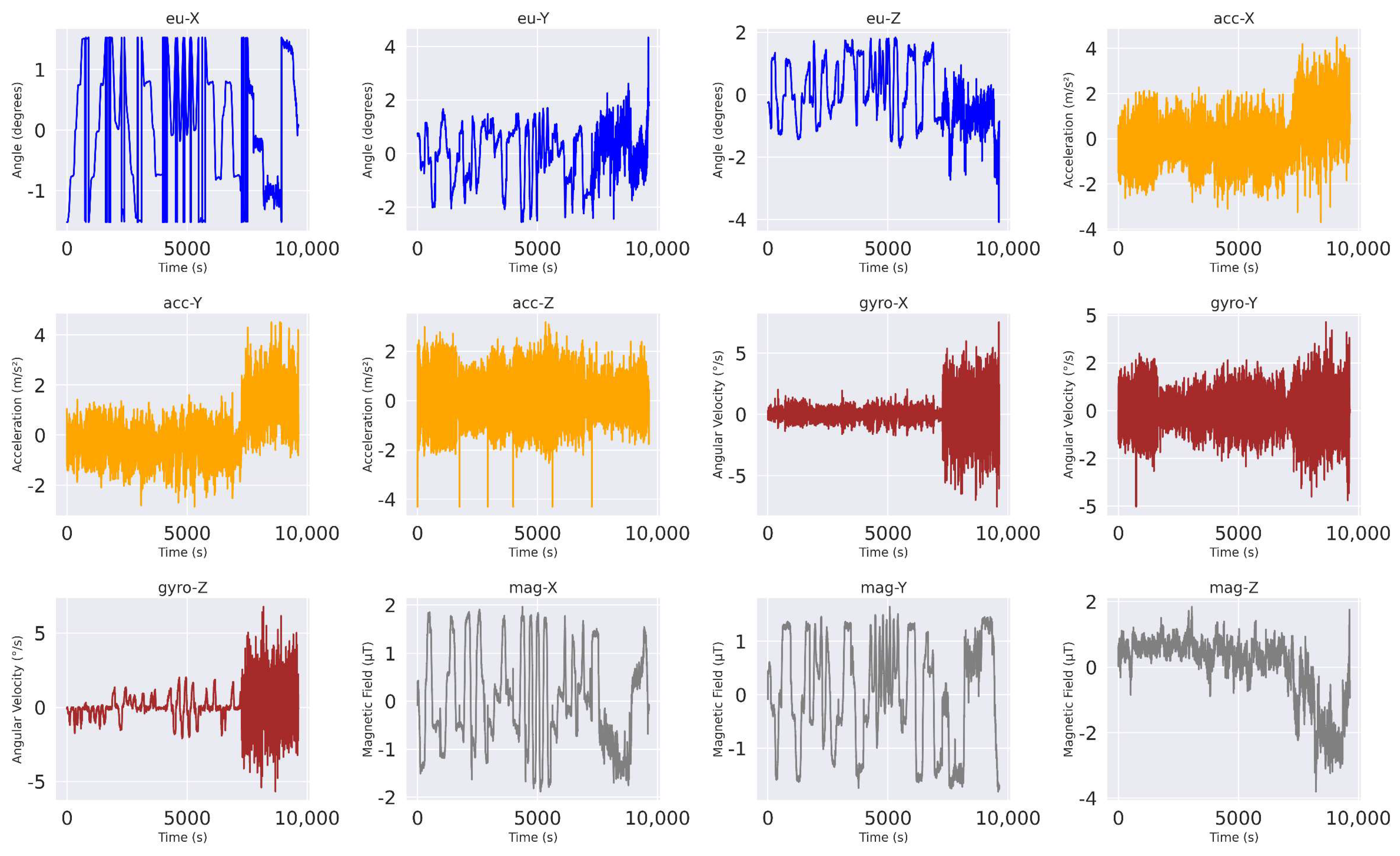
2.3. Data Description

Figure 6 displays a horizontal bar chart representing the count of different output classes, labeled from 0 to 6. Each bar indicates the number of instances for each class, with class 6 having the highest count of 2378 instances, followed by class 4 and class 5, both with 1640 instances. Class 2 has 1185 instances, class 3 has 1052 instances, class 1 has 1002 instances, and class 0 has the lowest count with 749 instances. The class distribution is notably uneven, with class 6 having the most instances and class 0 the least. This significant disparity in class counts can lead to model bias towards the more frequent classes. Models trained on these data might perform better on the more frequent classes, such as class 6, while potentially underperforming on the less frequent ones, such as class 0. To improve model performance, especially on the less frequent classes, techniques such as class weighting, oversampling the minority classes, or undersampling the majority classes could be employed. These methods help to balance the dataset, ensuring the model gives adequate attention to all classes. The chart highlights the importance of considering class imbalance when evaluating model performance. Accuracy might be misleading if it predominantly reflects performance in the more frequent classes. By addressing class imbalance, a fair and robust model training and evaluation process can be achieved, ensuring better generalization across all classes.

The graph in Figure 7 displays sensor data from a BNO055 sensor attached to a tractor, illustrating various aspects of its movement and orientation over time. The twelve subplots represent Euler angles (eu-X, eu-Y, eu-Z), accelerometer readings (acc-X, acc-Y, acc-Z), gyroscope readings (gyro-X, gyro-Y, gyro-Z), and magnetometer readings (mag-X, mag-Y, mag-Z). The Euler angles show the tractor’s orientation changes, indicating turns or shifts due to uneven terrain. Accelerometer readings reflect the tractor’s acceleration along three axes, with steady values indicating consistent movement and spikes, suggesting rapid changes in speed or direction. Gyroscope data reveal the tractor’s angular velocity, with high values indicating sharp turns. Magnetometer readings provide information on the tractor’s heading relative to the Earth’s magnetic field, with significant changes indicating direction shifts. Together, these plots offer a comprehensive view of the tractor’s movement patterns and responses to various driving conditions.

Exploratory Data Analysis (EDA) is crucial for understanding the distribution and characteristics of the dataset, and it involves various techniques to uncover underlying patterns and relationships. A correlation matrix is a useful tool for determining the magnitude and direction of linear associations between different variables, offering valuable insights into the possibility of multicollinearity. Boxplots are generated for each feature to visualize their distributions and identify outliers, which can significantly impact model performance. Scatter matrices plot the pairwise relationships between numeric features, offering a comprehensive view of how different sensor readings interact. Violin plots combine boxplot and density plot features, illustrating the data distribution’s shape and spread, while pair plots provide a detailed look at the bivariate relationships between features, highlighting clusters and correlations. These EDA techniques collectively enhance the understanding of the dataset, guiding the selection of appropriate preprocessing steps and machine learning models, ultimately leading to more robust and accurate predictions.

Figure 8 shows a series of boxplots representing sensor data from a BNO055 sensor on a tractor, illustrating the distribution, central tendency, and variability of the data. The Euler angles (eu-X, eu-Y, eu-Z) display medians around 200, 0, and 0, respectively, with interquartile ranges (IQRs) indicating the spread of the data and outliers highlighting variations. The accelerometer readings (acc-X, acc-Y, acc-Z) show medians near 0 for acc-X and acc-Y and around 9.5 for acc-Z, with IQRs, indicating the spread and several outliers showing deviations. Gyroscope readings (gyro-X, gyro-Y, gyro-Z) have medians close to 0, with IQRs from approximately −5 to 5 for gyro-X and gyro-Y, and −10 to 10 for gyro-Z, all with numerous outliers indicating fluctuations in rotation rates. Magnetometer readings (mag-X, mag-Y, mag-Z) also have medians near 0, with varying IQRs and several outliers, indicating variability in the magnetic field strength.

These boxplots collectively provide a comprehensive view of the tractor’s movement patterns and environmental conditions. While outliers were detected in the sensor data, they were retained in this analysis due to their real-world significance. These outliers correspond to significant changes in the terrain contour, which are critical for accurate surface recognition. Previous studies have demonstrated that removing outliers in scenarios involving complex surface interactions can lead to a reduction in predictive accuracy, as these outliers often represent valuable information about abrupt changes in the environment [34,35]. Therefore, removing them could result in a loss of essential data, which would compromise the system’s ability to adapt to rapidly changing surface conditions. Thus, retaining outliers was crucial for maintaining the robustness and accuracy of surface prediction in this study.

The correlation matrix (Figure 9) of the BNO055 sensor data for tractor movement offers useful insights into the interrelationships between different sensor readings and the objective variable. Notably, there are strong positive correlations between acceleration measurements, acc-X, acc-Y, and acc-Z, suggesting that these accelerations tend to increase or decrease together, likely reflecting coordinated tractor movements. The Euler angles, particularly eu-X and eu-Z, show a positive correlation (0.2), indicating some level of alignment or similar orientation changes in these axes. Interestingly, mag-Y and mag-Z have a strong negative correlation (−0.6), implying that changes in the magnetic field strength along the Y-axis are inversely related to changes along the Z-axis, likely due to the tractor’s orientation relative to the Earth’s magnetic field.

Regarding the target variable, there are moderate positive correlations with acc-Y (0.4), acc-Z (0.4), and mag-Z (0.4), indicating that these measurements are somewhat predictive of the target state or condition of the tractor. This suggests that the target variable is influenced by both acceleration and magnetic field strength. Conversely, the gyro data (gyro-X, gyro-Y, gyro-Z) show little to no correlation with the target variable, implying that angular velocity measurements may not be as critical in determining the target state.

The pair plot (Figure 10) of the BNO055 sensor data for tractor movement reveals several insightful patterns and relationships among the variables. The Euler angles (eu-X, eu-Y, eu-Z) show a cyclical relationship, especially between eu-X and eu-Y, indicating that the tractor frequently assumes certain rotational positions. The acceleration data (acc-X, acc-Y, acc-Z) demonstrate independent variations across different axes, with acc-Y showing more variation. Gyroscope readings (gyro-X, gyro-Y, gyro-Z) indicate significant spread, reflecting the tractor’s variable angular velocities. The magnetometer data (mag-X, mag-Y, mag-Z) reveal strong relationships, likely influenced by the tractor’s orientation relative to the Earth’s magnetic field. The output variable, which appears to be categorical, shows clear clusters when compared with the sensor data, suggesting strong influences from the tractor’s orientation and movement states. The observed multimodal distributions and independent variations among sensor readings offer opportunities for operational state identification, anomaly detection, and feature engineering. These insights can enhance the analysis and efficiency of tractor operations and support the development of predictive models for agricultural tasks.

Figure 11 shows a series of violin plots representing BNO055 sensor data from a tractor, categorized by different targets (likely different types of movements or conditions labeled from 0 to 6). The plots combine aspects of boxplots and density plots, revealing the distribution and probability density of the data. The Euler angles (eu-X, eu-Y, eu-Z) and accelerometer readings (acc-X, acc-Y, acc-Z) show varying distributions across targets, indicating differences in orientation and acceleration patterns for each movement or condition. Gyroscope readings (gyro-X, gyro-Y, gyro-Z) also display varied densities, suggesting distinct rotational rates around each axis depending on the target. Magnetometer readings (mag-X, mag-Y, mag-Z) show differences in magnetic field strength distributions, reflecting varying environmental conditions. These violin plots provide a comprehensive view of how the tractor’s sensor data changes with different targets, offering insights into the tractor’s movement patterns and responses to different conditions.

Table 2. Dataset distribution.

	eu-X	eu-Y	eu-Z	acc-X	acc-Y	acc-Z	gyro-X	gyro-Y	gyro-Z	mag-X	mag-Y	mag-Z
count	9646	9646	9646	9646	9646	9646	9646	9644	9644	9644	9644	9644
mean	179.46	−3.51	1.56	−0.49	−1.09	9.49	0.01	0.03	0.57	2.05	2.15	−3.32
std	117.85	4.68	5.98	0.83	1.04	2.20	6.61	11.80	11.26	24.25	24.90	5.53
min	0.00	−15.50	−22.87	−3.58	−4.08	0.00	−49.87	−59.43	−63.43	−43.68	−43.00	−24.37
25%	84.12	−6.87	−3.00	−1.07	−1.85	7.94	−2.43	−7.62	−3.31	−15.75	−17.51	−4.50
50%	181.31	−2.93	0.50	−0.51	−1.22	9.40	0.00	0.18	0.062	0.00	3.37	−1.25
75%	272.62	0.12	7.68	0.02	−0.49	10.99	2.37	7.75	4.87	18.25	24.75	0.18
max	360.00	16.81	12.56	3.25	3.62	16.52	49.87	54.81	76.75	49.68	43.00	6.87

presents the distribution of values from the dataset used in this study. The provided data represent summary statistics of various measurements from a BNO055 sensor on a tractor, including Euler angles (eu-X, eu-Y, eu-Z), accelerometer readings (acc-X, acc-Y, acc-Z), gyroscope readings (gyro-X, gyro-Y, gyro-Z), and magnetometer readings (mag-X, mag-Y, mag-Z). The Euler angles show significant variation in the tractor’s rotation and orientation. The eu-X angle has a mean of 179.46 with a wide range from 0 to 360 degrees, indicating substantial rotation around the X-axis. The eu-Y angle has a mean of −3.51 and ranges from −15.50 to 16.81 degrees, suggesting a slight backward tilt. The eu-Z angle shows a mean of 1.56 and ranges from −22.87 to 12.56 degrees, reflecting changes in the yaw or heading.

The accelerometer data provide information about the acceleration patterns of the tractor. The acceleration reading along the X-axis has a mean of −0.49 and a standard deviation of 0.83, indicating a minor deceleration. The acc-Y reading has a mean of −1.09, indicating a slight leftward tilt. The acc-Z reading, with a mean of 9.49, is close to the acceleration due to gravity, confirming that the Z-axis is aligned vertically. The gyroscope readings reveal significant rotational movements. The gyro-X, gyro-Y, and gyro-Z readings have means close to zero, with high standard deviations and wide ranges, indicating that the tractor experiences considerable rotational speeds around all three axes, especially in the Y and Z axes. This suggests dynamic rotational behavior during the tractor’s movement. The magnetometer readings show high variability in the magnetic field strengths along all axes. The mag-X, mag-Y, and mag-Z readings have means of 2.05, 2.15, and −3.32, respectively, with significant standard deviations and wide ranges. This suggests that the tractor operates in an environment with varying magnetic field strengths, likely due to different terrains or surrounding magnetic sources. Overall, these summary statistics provide a comprehensive understanding of the tractor’s dynamic behavior and environmental interactions, highlighting areas of significant movement and variability.

3. Results

This study aimed to enhance the navigation capabilities of autonomous tractors by predicting surface types using BNO055 IMU sensor data. To determine the balance of the training and testing data, a histogram is used, as shown in Figure 12. The image presents histograms of BNO055 sensor data from a tractor, separated into training (blue) and testing (green) datasets for various measurements: Euler angles (eu-X, eu-Y, eu-Z), accelerometer readings (acc-X, acc-Y, acc-Z), gyroscope readings (gyro-X, gyro-Y, gyro-Z), and magnetometer readings (mag-X, mag-Y, mag-Z). Each pair of histograms compares the distribution of values between the training and testing sets. The Euler angles and accelerometer readings generally show similar distributions between training and testing sets, indicating consistency in these measurements across different conditions. However, some measurements, particularly the magnetometer readings (mag-X, mag-Y, mag-Z), exhibit more variability and different distribution shapes between the datasets, suggesting potential differences in the magnetic field or environmental conditions during the training and testing periods. These histograms provide a visual comparison of the data distributions, highlighting areas where the training and testing sets align or differ, which can be crucial for understanding the model’s performance and generalizability.

Figure 13 exhibits confusion matrices for different machine learning models, assessing their performance on a classification problem. Each matrix presents a juxtaposition of the true class labels and the expected class labels. The evaluated models consist of Logistic Regression, K-Neighbors, SVC (Support Vector Classifier), Decision Tree, Random Forest, Gradient Boosting, AdaBoost, and XGBoost classifier. The Logistic Regression model shows a relatively dispersed distribution of predictions, with many misclassifications across different classes. For instance, while the model correctly predicts 99 instances of class 0, it also incorrectly classifies 177 instances as class 1, 30 as class 2, and 39 as class 3. The diagonal values are reasonably high, indicating a fair number of correct predictions (e.g., 684 for class 1 and 665 for class 5), but the off-diagonal values reveal significant misclassification.

The K-Neighbors classifier demonstrates high accuracy for certain classes, such as 744 correct predictions for class 0 and 1143 for class 2. However, it struggles with other classes, like class 3, where it misclassifies 29 instances as class 4 and 69 as class 5. Despite these misclassifications, the overall performance is decent, with a good number of correct predictions across the majority of classes. The SVC model shows a strong concentration of correct predictions along the diagonal, such as 742 correct predictions for class 0 and 1133 for class 2. Misclassifications are present but fewer compared to Logistic Regression, indicating better performance. For example, there are 45 misclassifications of class 3 as class 4 and 25 of class 4 as class 5, but overall, the SVC performs well.

The Decision Tree classifier has high values along the diagonal, indicating strong correct classification rates for many classes, such as 723 for class 0 and 1131 for class 2. However, several misclassifications suggest potential overfitting. For instance, class 3 has 36 instances misclassified as class 4 and 57 as class 5, showing that the model might be capturing noise in the training data. Random Forest shows high accuracy with a strong diagonal presence and fewer misclassifications. It correctly predicts 740 instances of class 0, 1179 of class 2, and 1601 of class 5, indicating robust performance across most classes. Misclassifications are minimal, with only a few instances such as class 3 having 25 misclassified as class 4.

The Gradient Boosting classifier demonstrates high performance with clear diagonal values and minimal off-diagonal misclassifications. It correctly predicts 733 instances of class 0, 1199 of class 2, and 1575 of class 5, showing robust performance and good prediction accuracy across most classes. Misclassifications, like 27 instances of class 4 being predicted as class 5, are relatively rare. AdaBoost shows mixed performance with several off-diagonal misclassifications, indicating struggles with certain classes. For example, class 0 has 154 correct predictions but 228 are misclassified as class 1 and 120 as class 2. However, there are also strong correct predictions for several classes, such as 679 for class 2 and 445 for class 5. XGBoost demonstrates high performance with strong diagonal values and minimal misclassifications. It correctly predicts 740 instances of class 0, 1171 of class 2, and 1608 of class 5. Misclassifications are few, with some instances, like class 4, having 17 misclassified as class 5, but overall, XGBoost shows good accuracy and generalization.

High-performance models such as Gradient Boosting, Random Forest, and XGBoost classifiers show strong performance with high accuracy and minimal misclassifications. For instance, XGBoost correctly predicts 1608 instances of class 5 with very few errors. Moderate performance models, like SVC and K-Neighbors, also perform well but have slightly more misclassifications, such as SVC misclassifying 32 instances of class 3 as class 4. Lower performance models, like Logistic Regression and AdaBoost, show higher misclassification rates, with Logistic Regression misclassifying 177 instances of class 0 as class 1, indicating more struggles with the classification task. Ensemble methods like Random Forest, Gradient Boosting, and XGBoost generally show better performance and robustness, providing better accuracy and generalization across different classes.

Table 3. Prediction accuracy based on dataset dividing type.

ML	K-Fold Cross-Validation	Random State (80/20)
LR	0.5354623361705697	0.5598755832037325
KNN	0.902738234288185	0.9015033696215656
SVC	0.921713247678478	0.9248315189217211
DT	0.9539603539769708	0.9574909279419388
RF	0.9850687475935114	0.9875583203732504
GB	0.963190084084588	0.9606013478486263
ADAB	0.4706558985048043	0.44841886988076723
XGB	0.9873498297443046	0.9885951270088128

presents the accuracy results of various machine learning models, evaluated using both K-Fold Cross-Validation and a Random State (80/20) split. For Logistic Regression (LR), the accuracy is relatively low, with K-Fold Cross-Validation yielding 0.5355 and the Random State split slightly higher at 0.5599. This indicates that Logistic Regression may not be the best choice for this classification task, as its performance is just above 50%. One of the key reasons for this underperformance is that Logistic Regression is a linear model, and it assumes that the relationship between the features and the target variable is linear. In the case of surface type prediction using IMU sensor data, the relationship between the features (e.g., acceleration, gyroscope, and magnetometer readings) and the target surface types is likely to be highly nonlinear and complex. Therefore, more sophisticated models that can capture these nonlinear interactions, such as K-Neighbor (KNN), the Support Vector Classifier (SVC), or ensemble methods, like Random Forest and XGBoost, perform significantly better. The K-Neighbor (KNN) classifier performs well, achieving over 90% accuracy in both evaluation methods (0.9027 for K-Fold and 0.9015 for Random State). The consistency between these accuracies suggests reliable performance across different data splits. Similarly, the Support Vector Classifier (SVC) demonstrates strong performance with accuracies of 0.9217 and 0.9248 for K-Fold and Random State, respectively, indicating good generalization and robustness.

The Decision Tree (DT) model shows high accuracy, around 95%, with K-Fold yielding 0.9540 and Random State 0.9575. This high accuracy indicates that the model effectively captures the patterns in the data. The slight improvement in the Random State split suggests a good fit for the model. Random Forest (RF) exhibits excellent performance with accuracies of 0.9851 for K-Fold and 0.9876 for Random State, confirming its robustness and effectiveness in handling the classification task. Gradient Boosting (GB) maintains high accuracy, approximately 96%, with a slight variation between K-Fold (0.9632) and Random State (0.9606). This consistency reflects the model’s strong predictive power. In contrast, AdaBoost (ADAB) shows lower accuracy, below 50%, with K-Fold at 0.4707 and Random State at 0.4484. The performance of AdaBoost is limited in this task due to its sensitivity to noisy data and outliers. Since AdaBoost works by combining weak learners in a sequential manner, it gives more weight to misclassified data points in each iteration. This can lead to poor performance in datasets where the relationships between features and the target variable are complex or nonlinear, as is the case with IMU sensor data. Moreover, AdaBoost tends to overemphasize noisy or difficult-to-classify instances, which can result in a lower overall accuracy. The slight decrease in the Random State split suggests limited generalization ability, further indicating that AdaBoost struggles with this particular classification task.

XGBoost (XGB) achieves the highest accuracy among the models, around 98.7%, with consistent results in both evaluation methods (0.9873 for K-Fold and 0.9886 for Random State). This performance highlights XGBoost’s superiority in handling the dataset, offering excellent accuracy and robustness. Overall, the high-performing models are Random Forest (RF) and XGBoost (XGB), with accuracies around 98.5% to 98.8%, indicating their strong capabilities in the classification task. Moderate-performing models include the SVC, Decision Tree, and Gradient Boosting, with accuracies ranging from 92% to 96%. Logistic Regression and AdaBoost show significantly lower accuracies, with AdaBoost performing the worst, suggesting that these models are less suitable for this task. The consistency of models like KNN, SVC, RF, and XGB across both evaluation methods indicates they are reliable and robust, making ensemble methods, particularly XGBoost and Random Forest, the best performers for this classification task.

Figure 14 displays the ROC (Receiver Operating Characteristic) curves for several machine learning models, including Logistic Regression, K-Neighbors, SVC, Decision Tree, Random Forest, Gradient Boosting, AdaBoost, and XGBoost classifier. Each subplot demonstrates the sensitivity (true positive rate) versus the false positive rate for each class, with the AUC (area under the curve) values reflecting the performance of the model. Greater AUC values indicate superior model performance. Logistic Regression demonstrates moderate effectiveness, with Area Under the Curve (AUC) values ranging from 0.75 to 0.88. The algorithms K-Neighbors, SVC, Decision Tree, Random Forest, Gradient Boosting, and XGBoost demonstrate exceptional performance since most classes have AUCs near 1.0, showing a high level of discriminative ability. AdaBoost has the lowest performance, with AUCs between 0.68 and 0.86, indicating weaker classification ability. Overall, the ROC curves highlight that ensemble methods like Random Forest, Gradient Boosting, and XGBoost achieve superior performance, making them more effective for this classification task.

Based on the experimental design proposed earlier, testing was conducted using the same scenarios as those used for data collection in training and testing. The Random Forest model was chosen to be embedded into the Arduino Nano 33 BLE for real-time prediction because micromlgen supports converting the Random Forest models from joblib to the RandomForest.c format. Real-time field testing was carried out by comparing the predictions made by the embedded model on the Nano 33 BLE with the actual scenarios run.

Table 4. Real-time surface recognition accuracy.

Scenario	Track	Surface	Accuracy (%)
Scenario 1	Around	Asphalt	96.21
Scenario 2	Around	Gravel	98.51
Scenario 3	Zigzag	Gravel	98.94
Scenario 4	Around	Concrete + Gravel	96.09
Scenario 5	Zigzag	Concrete + Gravel	96.44
Scenario 6	Around	Soil + Grass	98.52
Scenario 7	Zigzag	Soil + Grass	97.97
Average Accuracy			97.53

presents the real-time testing results, with an average accuracy of 97.53% across the seven scenarios.

4. Discussion

The results indicate that ensemble approaches, specifically Random Forest and XGBoost, exhibit superior performance compared to other models in forecasting surface types using IMU sensor data. This high performance is consistent with previous research, which has shown that ensemble methods excel in handling complex classification tasks due to their ability to combine multiple weak learners into a strong predictor. In comparison to earlier studies that utilized basic classifiers, such as Logistic Regression and SVMs, the results indicate a marked improvement in accuracy. For instance, while traditional approaches, like Logistic Regression, achieved accuracies around 50–60%, the use of Random Forest and XGBoost achieved accuracies close to 99%. This suggests that these models are more capable of capturing the nuanced patterns in the sensor data that correspond to different surface types.

Moreover, the Random Forest and XGBoost models demonstrate exceptional discriminative ability, as evidenced by their high ROC-AUC values approaching 1.0. Similar studies have shown the importance of accurate terrain classification for autonomous vehicles. For example, in the work of [36], which focused on surface-type prediction for autonomous vehicles using sensor fusion, the ensemble methods outperformed traditional machine learning models. Random Forest achieved higher accuracy in predicting transitions between gravel and asphalt surfaces, a result that is consistent with the findings of this study. Likewise, the research by [37] demonstrated that ensemble learning methods, such as Gradient Boosting, significantly improved surface recognition, particularly in handling real-world scenarios where terrain transitions affected vehicle stability and speed regulation.

The strong performance of these models in this study can be attributed to their ability to manage feature interactions and their inherent resilience to overfitting due to their ensemble structure. The implications of these findings are significant for the development of autonomous tractors. Accurate surface type prediction ensures that the tractor can adjust its navigation strategy according to the terrain, improving operational efficiency and safety. For instance, recognizing a transition from asphalt to gravel can prompt the tractor to adjust its speed and handling characteristics to prevent slipping or instability. This aligns with research by [38], who demonstrated that precise surface recognition could help autonomous agricultural vehicles adjust their speed in real time, significantly reducing the risk of operational errors during surface transitions.

One of the key limitations of earlier studies was the inadequate performance in diverse real-world environments, often resulting in misclassifications. This study addresses this limitation by leveraging advanced ensemble techniques that demonstrate high accuracy and robustness across different terrains. This advancement provides a more reliable foundation for real-world applications, enhancing the practical deployment of autonomous tractors. In conclusion, the research convincingly demonstrates the superiority of ensemble methods, particularly Random Forest and XGBoost, in surface-type prediction using IMU sensor data. The high accuracy and robustness of these models underscore their potential to significantly enhance the navigation capabilities of autonomous tractors. By addressing the limitations of previous approaches, this study contributes to the development of more reliable and efficient autonomous agricultural systems that are capable of adapting to diverse environmental conditions without human assistance.

5. Conclusions

This study makes a significant contribution to the field of autonomous navigation by showing that employing BNO055 IMU sensor data is useful in predicting terrain types. This, in turn, improves the operational capabilities of autonomous tractors. Through the utilization of sophisticated ensemble learning methods, like Random Forest and XGBoost, unparalleled levels of accuracy have been attained in the categorization of surface types, greatly surpassing the performance of conventional models. The findings offer a robust solution to the critical challenge of surface recognition in autonomous vehicles. The superior performance of Random Forest and XGBoost in handling complex, real-world data underscores their potential for practical applications in agriculture, where diverse terrains are common. This research provides a scientific basis for deploying these advanced models in autonomous tractors, ensuring they can navigate various surfaces with greater efficiency and safety.

While Random Forest and XGBoost show strong overall performance, it is important to consider their potential limitations in extreme or edge cases. For instance, both methods might encounter challenges in recognizing highly similar or ambiguous surface types, which can affect classification accuracy in complex environments. In practical applications, issues such as varying sensor data quality, changes in environmental conditions, and hardware limitations on tractors could impact the models’ performance.

Looking ahead, future work will focus on leveraging the predictive capabilities of these models to automatically control the speed of the tractor in real time. This development aims to further enhance the adaptability and efficiency of autonomous tractors by enabling real-time adjustments in response to changing surface conditions. Additionally, exploring the integration of other sensor data, such as LIDAR or visual inputs, may further improve the models’ predictive accuracy and robustness.

Overall, this research lays the groundwork for improving surface recognition in autonomous tractors and opens the door to more dependable and effective agricultural automation. This work advances autonomous navigation technology by surpassing the shortcomings of prior methods and reaching high predicted accuracy, with exciting implications for the development of smart farming in the future.

References

1. Qu, J.; Zhang, Z.; Qin, Z.; Guo, K.; Li, D. Applications of Autonomous Navigation Technologies for Unmanned Agricultural Tractors: A Review. Machines 2024, 12, 218. [Google Scholar] [CrossRef]
2. Xie, B.; Jin, Y.; Faheem, M.; Gao, W.; Liu, J.; Jiang, H.; Cai, L.; Li, Y. Research Progress of Autonomous Navigation Technology for Multi-Agricultural Scenes. Comput. Electron. Agric. 2023, 211, 107963. [Google Scholar] [CrossRef]
3. Gil, G.; Casagrande, D.E.; Cortés, L.P.; Verschae, R. Why the Low Adoption of Robotics in the Farms? Challenges for the Establishment of Commercial Agricultural Robots. Smart Agric. Technol. 2023, 3, 100069. [Google Scholar] [CrossRef]
4. Shi, J.; Bai, Y.; Diao, Z.; Zhou, J.; Yao, X.; Zhang, B. Row Detection BASED Navigation and Guidance for Agricultural Robots and Autonomous Vehicles in Row-Crop Fields: Methods and Applications. Agronomy 2023, 13, 1780. [Google Scholar] [CrossRef]
5. Vrochidou, E.; Oustadakis, D.; Kefalas, A.; Papakostas, G.A. Computer Vision in Self-Steering Tractors. Machines 2022, 10, 129. [Google Scholar] [CrossRef]
6. Roshanianfard, A.; Noguchi, N.; Okamoto, H.; Ishii, K. A Review of Autonomous Agricultural Vehicles (The Experience of Hokkaido University). J. Terramech. 2020, 91, 155–183. [Google Scholar] [CrossRef]
7. Samatas, G.G.; Pachidis, T.P. Inertial Measurement Units (IMUs) in Mobile Robots over the Last Five Years: A Review. Designs 2022, 6, 17. [Google Scholar] [CrossRef]
8. Oliver, M.A. Progress in Precision Agriculture Series Editor; Springer International Publishing: Cham, Switzerland, 2021. [Google Scholar]
9. Loukatos, D.; Petrongonas, E.; Manes, K.; Kyrtopoulos, I.V.; Dimou, V.; Arvanitis, K.G. A Synergy of Innovative Technologies towards Implementing an Autonomous Diy Electric Vehicle for Harvester-Assisting Purposes. Machines 2021, 9, 82. [Google Scholar] [CrossRef]
10. Yeong, D.J.; Velasco-hernandez, G.; Barry, J.; Walsh, J. Sensor and Sensor Fusion Technology in Autonomous Vehicles: A Review. Sensors 2021, 21, 2140. [Google Scholar] [CrossRef]
11. Zhao, W.; Li, T.; Qi, B.; Nie, Q.; Runge, T. Terrain Analytics for Precision Agriculture with Automated Vehicle Sensors and Data Fusion. Sustainability 2021, 13, 2905. [Google Scholar] [CrossRef]
12. Lu, E.; Xue, J.; Chen, T.; Jiang, S. Robust Trajectory Tracking Control of an Autonomous Tractor-Trailer Considering Model Parameter Uncertainties and Disturbances. Agriculture 2023, 13, 869. [Google Scholar] [CrossRef]
13. Adab, H.; Morbidelli, R.; Saltalippi, C.; Moradian, M.; Ghalhari, G.A.F. Machine Learning to Estimate Surface Soil Moisture from Remote Sensing Data. Water 2020, 12, 3223. [Google Scholar] [CrossRef]
14. Ge, G.; Shi, Z.; Zhu, Y.; Yang, X.; Hao, Y. Land Use/Cover Classification in an Arid Desert-Oasis Mosaic Landscape of China Using Remote Sensed Imagery: Performance Assessment of Four Machine Learning Algorithms. Glob. Ecol. Conserv. 2020, 22, e00971. [Google Scholar] [CrossRef]
15. Sharma, A.; Jain, A.; Gupta, P.; Chowdary, V. Machine Learning Applications for Precision Agriculture: A Comprehensive Review. IEEE Access 2021, 9, 4843–4873. [Google Scholar] [CrossRef]
16. Mohinur Rahaman, M.; Azharuddin, M. Wireless Sensor Networks in Agriculture through Machine Learning: A Survey. Comput. Electron. Agric. 2022, 197, 106928. [Google Scholar] [CrossRef]
17. Singh, A.; Nawayseh, N.; Singh, H.; Dhabi, Y.K.; Samuel, S. Internet of Agriculture: Analyzing and Predicting Tractor Ride Comfort through Supervised Machine Learning. Eng. Appl. Artif. Intell. 2023, 125, 106720. [Google Scholar] [CrossRef]
18. Buya, S.; Tongkumchum, P.; Owusu, B.E. Modelling of Land-Use Change in Thailand Using Binary Logistic Regression and Multinomial Logistic Regression. Arab. J. Geosci. 2020, 13, 437. [Google Scholar] [CrossRef]
19. Mazumder, B.; Khan, M.S.I.; Mohi Uddin, K.M. Biorthogonal Wavelet Based Entropy Feature Extraction for Identification of Maize Leaf Diseases. J. Agric. Food Res. 2023, 14, 100756. [Google Scholar] [CrossRef]
20. Kok, Z.H.; Mohamed Shariff, A.R.; Alfatni, M.S.M.; Khairunniza-Bejo, S. Support Vector Machine in Precision Agriculture: A Review. Comput. Electron. Agric. 2021, 191, 106546. [Google Scholar] [CrossRef]
21. Reddy, K.S.P.; Roopa, Y.M.; Kovvada Rajeev, L.N.; Nandan, N.S. IoT Based Smart Agriculture Using Machine Learning. In Proceedings of the Second International Conference on Inventive Research in Computing Applications (ICIRCA-2020), Coimbatore, India, 15–17 July 2020; pp. 130–134. [Google Scholar]
22. Wang, H.; Yilihamu, Q.; Yuan, M.; Bai, H.; Xu, H.; Wu, J. Prediction Models of Soil Heavy Metal(Loid)s Concentration for Agricultural Land in Dongli: A Comparison of Regression and Random Forest. Ecol. Indic. 2020, 119, 106801. [Google Scholar] [CrossRef]
23. Huber, F.; Yushchenko, A.; Stratmann, B.; Steinhage, V. Extreme Gradient Boosting for Yield Estimation Compared with Deep Learning Approaches. Comput. Electron. Agric. 2022, 202, 107346. [Google Scholar] [CrossRef]
24. Li, Y.; Guo, Y.; Gong, L.; Liu, C. Harvesting Route Detection and Crop Height Estimation Methods for Lodged Farmland Based on AdaBoost. Agriculture 2023, 13, 1700. [Google Scholar] [CrossRef]
25. Mariadass, D.A.L.; Moung, E.G.; Sufian, M.M.; Farzamnia, A. Extreme Gradient Boosting (XGBoost) Regressor and Shapley Additive Explanation for Crop Yield Prediction in Agriculture. In Proceedings of the 2022 12th International Conference on Computer and Knowledge Engineering, ICCKE 2022, Mashhad, Iran, 17–18 November 2022; Institute of Electrical and Electronics Engineers Inc.: New York, NY, USA, 2022; pp. 219–224. [Google Scholar]
26. Grygar, T.M.; Radojičić, U.; Pavlů, I.; Greven, S.; Nešlehová, J.G.; Tůmová, Š.; Hron, K. Exploratory Functional Data Analysis of Multivariate Densities for the Identification of Agricultural Soil Contamination by Risk Elements. J. Geochem. Explor. 2024, 259, 107416. [Google Scholar] [CrossRef]
27. Dash, C.S.K.; Behera, A.K.; Dehuri, S.; Ghosh, A. An Outliers Detection and Elimination Framework in Classification Task of Data Mining. Decis. Anal. J. 2023, 6, 100164. [Google Scholar] [CrossRef]
28. Kebonye, N.M. Exploring the Novel Support Points-Based Split Method on a Soil Dataset. Measurement 2021, 186, 110131. [Google Scholar] [CrossRef]
29. Lyu, Z.; Yu, Y.; Samali, B.; Rashidi, M.; Mohammadi, M.; Nguyen, T.N.; Nguyen, A. Back-Propagation Neural Network Optimized by K-Fold Cross-Validation for Prediction of Torsional Strength of Reinforced Concrete Beam. Materials 2022, 15, 1477. [Google Scholar] [CrossRef]
30. Vu, H.L.; Ng, K.T.W.; Richter, A.; An, C. Analysis of Input Set Characteristics and Variances on K-Fold Cross Validation for a Recurrent Neural Network Model on Waste Disposal Rate Estimation. J. Environ. Manag. 2022, 311, 114869. [Google Scholar] [CrossRef]
31. Chicco, D.; Jurman, G. The Matthews Correlation Coefficient (MCC) Should Replace the ROC AUC as the Standard Metric for Assessing Binary Classification. BioData Min. 2023, 16, 4. [Google Scholar] [CrossRef]
32. Valero-Carreras, D.; Alcaraz, J.; Landete, M. Comparing Two SVM Models through Different Metrics Based on the Confusion Matrix. Comput. Oper. Res. 2023, 152, 106131. [Google Scholar] [CrossRef]
33. Rachakonda, A.R.; Bhatnagar, A. ARatio: Extending Area under the ROC Curve for Probabilistic Labels. Pattern Recognit. Lett. 2021, 150, 265–271. [Google Scholar] [CrossRef]
34. Zou, M.; Djokic, S.Z. A Review of Approaches for the Detection and Treatment of Outliers in Processing Wind Turbine and Wind Farm Measurements. Energies 2020, 13, 4228. [Google Scholar] [CrossRef]
35. Ribeiro, R.P.; Moniz, N. Imbalanced Regression and Extreme Value Prediction. Mach. Learn. 2020, 109, 1803–1835. [Google Scholar] [CrossRef]
36. Veloso, M. Machine Learning for Autonomous Vehicle Road Condition Analysis. J. AI Healthc. Med. 2023, 3, 141–159. [Google Scholar]
37. Jamal, A.; Zahid, M.; Tauhidur Rahman, M.; Al-Ahmadi, H.M.; Almoshaogeh, M.; Farooq, D.; Ahmad, M. Injury Severity Prediction of Traffic Crashes with Ensemble Machine Learning Techniques: A Comparative Study. Int. J. Inj. Contr. Saf. Promot. 2021, 28, 408–427. [Google Scholar] [CrossRef] [PubMed]
38. Reina, G.; Milella, A.; Rouveure, R.; Nielsen, M.; Worst, R.; Blas, M.R. Ambient Awareness for Agricultural Robotic Vehicles. Biosyst. Eng. 2016, 146, 114–132. [Google Scholar] [CrossRef]
Figure 1. Research overview.
Agriculture 14 01557 g001
Figure 2. Small mobile tractor robot.
Agriculture 14 01557 g002
Figure 3. Real-time surface recognition diagram.
Agriculture 14 01557 g003
Figure 4. Satellite views of the locations for each scenario. The red line represents the path boundary or a specific area under observation. The green line indicates the path of the small tractor robot’s movement. The yellow dots denote the start and end points.
Agriculture 14 01557 g004
Figure 5. Experimental environment.
Agriculture 14 01557 g005
Figure 6. Count of different output classes.
Agriculture 14 01557 g006
Figure 7. Dataset distributions.
Agriculture 14 01557 g007
Figure 8. Boxplot dataset distributions.
Agriculture 14 01557 g008
Figure 9. Correlation matrix.
Agriculture 14 01557 g009
Figure 10. Dataset pair plots.
Agriculture 14 01557 g010
Figure 11. Dataset violin plots.
Agriculture 14 01557 g011
Figure 12. Training and testing dataset distribution.
Agriculture 14 01557 g012
Figure 13. Confusion matrix.
Agriculture 14 01557 g013
Figure 14. ROC and AUC graphs.
Agriculture 14 01557 g014