Coupling Coordination and Spatial–Temporal Evolution of the Water–Land–Ecology System in the North China Plain

Abstract

Exploring the coordination of agricultural water resources (W), cultivated land (L), and the ecoenvironment (E) system is crucial for sustainable agriculture in the North China Plain (NCP). However, the synergistic effects of this composite system remain unclear. Coupling coordination degrees (CCDs) of 53 cities in the NCP for the years 2011, 2015, and 2020 were evaluated using the TOPSIS model, and the coupling coordination model, combined with the analytic hierarchy process and entropy weight method. The evaluation results were further analyzed to identify obstacle factors. The findings reveal the following: (1) The comprehensive development level showed a fluctuating upward trend, with closeness values ranging from 0.418 to 0.574 in 2020, indicating an improvement of 14.6–52.3% compared to 2011. The coefficient of variation (CV) for each province rose from 12.65% in 2011 to 13.64% and subsequently declined to 9.12% by 2020. (2) Between 2011 and 2020, CCDs of the W–L–E composite system exhibited a consistent upward trend. In 2020, regions with intermediate or better coordination accounted for 34.0%, and were primarily located in Jiangsu Province, the southern part of Anhui Province, the northwestern part of Shandong Province, and the municipalities of Beijing and Tianjin. (3) In 2011 and 2015, significant obstacle factors included the water quality compliance rate and the per capita disposable income of rural residents, although these were not primary obstacles in 2020. The water supply modulus and multiple cropping index were major obstacle factors in 2011, 2015, and 2020. Developing water-appropriate cropping patterns based on regional water resource endowment is the essential path for the sustainable and coordinated development of water, land, and ecology in the NCP.

1. Introduction

Water and land resources are essential materials and natural resources for human survival [1], directly relating to food security and the sustainable development of agriculture [2]. The North China Plain constitutes 20.4% of the nation’s cultivated land, yet it is responsible for over 35% of the national grain yield, despite relying on a mere 6% of the country’s water resources [3]. Due to the mismatch of water and land resources, coupled with the extensive use of pesticides and chemical fertilizers, negative impacts have been imposed on the ecological environment, such as soil contamination, ecological regression, and water pollution [4,5,6]. Simultaneously, the excessive extraction of groundwater has resulted in the formation of the world’s largest groundwater cone of depression area [7]. With the rapid development of China’s economy and the ongoing promotion of urbanization, water and land resources are increasingly diverted to nonagricultural industries, leading to an annual average irrigation water shortage exceeding 3 × 10¹⁰ m³. Irrigation agriculture in the NCP faces severe challenges [8]. Therefore, scientifically assessing the coupling and coordination of the three subsystems—agricultural water resources, cultivated land, and ecological environment—and exploring potential obstacle factors are directly related to regional ecological balance and food security.

Many scholars have engaged in research to explore the interactions between water, land, and ecoenvironment, including the pairwise relationships between water and land, water and ecoenvironment, and land and ecoenvironment [9]. The Coupling Coordination Degree Model (CCDM) is a principal evolutionary framework employed for assessing interactions and the degree of coordination among subsystems and is widely utilized in various research fields [10,11,12]. Within the CCDM, the Coupling Coordination Degree (CCD) acts as a metric for gauging the evolution of a composite system toward a higher level of organization, indicative of sustainable development progress [13]. The coupling of water and land resources mainly focuses on balance or coupling coordination relationships [14,15], the optimal allocation of agricultural water and land [16,17], resource carrying capacity [18,19], and sustainable utilization [20]. Lv et al. [14] utilized the “Driving Force–Pressure–State–Impact–Response” (DPSIR) model to assess the interaction between water and land resources. Xie et al. [21] utilized the coupling coordination degree model to evaluate the coupling coordination relationship between land space development and the ecological environment of Henan Province. He and Wang [22] put forward a framework to assess trends in the water–land resource carrying capacity from the perspectives of the water–land resource supporting force and pressure, employing a decoupling model integrated with the ecological footprint concept and an index system.

As research deepens, studies on the integration of water and land resources with third systems—such as urbanization [23], rural settlement [24], food security [25], economic development [26], energy [27], and the ecological environment [28]—are increasing. Cheng et al. [28] analyzed the coupling coordination relationships of regional water and land resources and ecoenvironment systems with a focus on speed characteristics. Zhu et al. [29] utilized the Gini coefficient and a water–land congruence metric to examine the interrelationships within the water–land–food nexus across the principal grain-producing regions of the North China Plain over the period from 2000 to 2020. Research methods often include coupling coordination degree [28], matching coefficients [30], and linear and nonlinear programming [16,17,31], and encompass various scales such as administrative units [28], irrigation areas [32], river basins [15,33], and grid-based analyses [34].

In general, there are certain shortcomings in the existing studies on the CCD of the W–L–E system. Most previous studies have focused on the coordination of either water and land resources individually or two of the W–L–E systems. There is a scarcity of studies examining the coupling coordination relationship and obstacle factors of all three systems using microindicators. In addition, the current studies lack a coordinated analysis of the W–L–E system at the municipal level in the NCP. Accordingly, this paper constructs an integrated assessment framework named agricultural water resource carrying capacity, cultivated land use efficiency, and eco-environmental pressure. It examines the coupling and coordination characteristics in 53 cities across the years 2011, 2015, and 2020, and identifies the key obstacle factors. The findings are expected to provide valuable references and suggestions to optimize the use of agricultural water and cultivated land resources, and to promote the sustainable development of modern agriculture.

2. Materials and Methods

2.1. Study Area

The NCP, situated in the eastern region of China, spans latitudes 32°08′–40°24′ N and longitudes 112°50′–122°40′ E [35] (Figure 1). The total area is approximately 30 × 10⁴ km², including most or all of Beijing, Tianjin, Henan, Hebei, Shandong, Anhui, and Jiangsu provinces [36], with an average annual temperature of 14–15 °C and annual precipitation of 500–1000 mm [37]. Because it has sufficient light and heat and fertile land, it has become the most important agricultural, animal husbandry, and commodity grain base in China, as well as an important industrial manufacturing center and urban agglomeration center. The region includes 53 cities and has a population of over 250 million, with 67.79% of residents dependent on agriculture for their livelihoods [38].

2.2. Data Sources

Taking 2011, 2015, and 2020 as the evaluation years, 23 representative indicators were selected to evaluate the coupling coordination degree of the W–L–E system and subsystems in the NCP. The basic data for 53 cities came from the China Statistical Yearbook, China Statistical Yearbook on Environment, Statistical Bulletins of various provinces and cities, Agricultural Statistical Bulletins, Statistical Bulletins on National Economic and Social Development, and Water Resources Bulletins.

Table 1. An overview of the data used in this study.

Data Name	Year	Resolution/Data Level	Acquisition Source
DEM	2020	250 m	https://www.gscloud.cn/ accessed on 10 April 2022
China Statistical Yearbook	2011, 2015, 2020	Provincial level	https://www.stats.gov.cn/sj/ndsj/ accessed on 17 June 2022
China Statistical Yearbook on Environment	2011, 2015, 2020	Provincial level	https://www.mee.gov.cn/ accessed on 19 May 2023
Water Resources Bulletins	2011, 2015, 2020	Provincial level	http://szy.mwr.gov.cn/gbsj/index.html accessed on 24 June 2023
Statistical Bulletins on National Economic and Social Development	2011, 2015, 2020	Provincial and municipal levels	Provincial and municipal statistical departments accessed on 13 July 2023
Statistical Bulletins	2011, 2015, 2020	Provincial and municipal levels	Provincial and municipal statistical departments accessed on 21 September 2023

presents the sources of data utilized in this study. Individual missing values were supplemented by interpolation or the average method to ensure the accuracy and scientific nature of the data.

2.3. Methods

A proposed methodology for assessing the coupling coordination relationship of the W–L–E system includes the following procedures (Figure 2): (1) Screening and establishment of the system evaluation framework. (2) Determination of composite weights using the Analytic Hierarchy Process (AHP) and the Entropy Weight Method (EWM). (3) Application of the TOPSIS method (technique for order preference by similarity to ideal solution) to evaluate the development level of the W–L–E composite system and subsystems. (4) Assessment of the coupling coordination degree of the system with the coupling coordination model. (5) Diagnosis of the key obstacle factors to the composite system using the obstacle degree model. Data processing, analysis, and visualization were performed using Microsoft Excel 2019 (Microsoft Corp., Redmond, WA, USA), ArcGIS 10.2 (Environmental Systems Research Institute, Redlands, CA, USA), and Origin 2021 (OriginLab Corp., Northampton, MA, USA).

2.3.1. Index System Construction

The assessment and analysis of water and land resources, along with eco-environmental resources, are generally conducted through the establishment of evaluation index systems at various levels. Based on the structure of the composite system, it can be divided into three subsystems: the agricultural water resource carrying capacity subsystem (A1), the cultivated land use efficiency subsystem (A2), and the ecological environment pressure subsystem (A3). Here, A1 highlights the reliability of agricultural water resources, and A2 concentrates on the productivity of cultivated land. Indicators at the criterion and indicator layers were determined following the principles of scientific rigor, systematic approach, comparability, and accessibility, and with reference to numerous relevant studies [9,14,19,21,28,32,39,40,41]. As shown in

Table 2. Comprehensive evaluation index system.

Subsystem	Criterion	Indicator	Unit	Formula	Property
Agricultural water resource carrying capacity (A1)	Water saving (B1)	proportion of water-saving irrigation (C1)	%	Water-saving irrigation area/cultivated land area	Positive
	Water use (B2)	Proportion of agricultural water use (C2)	%	Agricultural water use/total water use	Negative
		Irrigation water use per area (C3)	m3/ha	Irrigation water use/effective irrigation area	Negative
		Cultivated land irrigation rate (C4)	%	Effective irrigation area/cultivated land area	Positive
		Water consumption per agricultural output value (C5)	m3/104 CNY	Agricultural water consumption /agricultural output value	Negative
	Water supply (B3)	Proportion of groundwater supply to total water supply (C6)	%	Groundwater supply/total water supply	Negative
		Proportion of groundwater supply to groundwater resources (C7)	%	Groundwater supply/groundwater volume	Negative
		Water supply modulus (C8)	m3/m2	Total water supply/total area	Positive
		Precipitation modulus (C9)	m3/m2	Total precipitation/total area	Positive
Cultivated land use efficiency (A2)	Economic benefits (B5)	Grain yield per ha (C10)	kg/ha	Grain yield/cultivated land area	Positive
		Output value per cultivated land area (C11)	104 CNY/ha	Agricultural output value/cultivated land area	Positive
		Agricultural output value per capita (C12)	104 CNY/capita	Agricultural output value/agricultural population	Positive
		Degree of agricultural mechanization (C13)	kw/ha	Total agricultural machinery power/cultivated land area	Positive
		Labor force per cultivated land area (C14)	people/ha	Agricultural population/cultivated land area	Positive
	Social benefits (B6)	Food safety coefficient (C15)	%	Grain yield per capita/400 kg	Positive
		Disposable income of rural residents per capita (C16)	104 CNY	Statistical data	Positive
		Cultivated land area per capita (C17)	ha/capita	Cultivated land area/total population	Positive
		Grain yield per capita (C18)	kg/capita	Grain yield/total regional population	Positive
Ecological environment pressure (A3)	Land (B7)	Multiple cropping index (C19)	%	Sown area of crops/cultivated land area	Negative
		Fertilizer utilization rate (C20)	kg/ha	Amount of fertilizer applied/cultivated land area	Negative
		Pesticide utilization rate (C21)	kg/ha	Amount of pesticide applied/cultivated land area	Negative
	Energy (B8)	Energy consumption rate (C22)	kw·h/104 CNY	Rural electricity use/agricultural output value	Negative
	Water (B9)	Water quality compliance rate (C23)	%	Statistical data	Positive

, a total of 23 different indicators were selected. Among these, indicators C1–C9 pertain to the supply, consumption, and conservation of agricultural water resources, with a particular emphasis on the proportion of groundwater in the water supply. Indicators C10–C18 cover the economic and social benefits derived from cultivated land use, highlighting the role of cultivated land in fostering agricultural and rural development. Indicators C19–C23 address cultivated land pressure, energy pressure, and water environment pressure, emphasizing the impact of agricultural water and soil resource utilization on the ecological environment.

2.3.2. AHP Method

The AHP is a Multicriteria Decision-Making (MCDM) method that integrates both qualitative and quantitative approaches to determine the weights of objectives. It assists decision-makers in addressing complex problems with multiple, inter-related subjective criteria and is widely applied in the fields of management and decision-making [42]. The main computational process is divided into four steps:

(a)

Construct a judgment matrix $A={\left(a_{ij}\right)}_{n\times \mathrm{n}}$, where $a_{ij}$ represents the quantified degree of importance of criterion $i$ relative to criterion $j$, using a scale of numbers from 1 to 9 and their reciprocals.

(b)

By employing the formula $Aw={\mathsf{\lambda }}_{max}w$, derive the maximum eigenvalue ${\mathsf{\lambda }}_{max}$ and its corresponding eigenvector $w$ of the judgment matrix $A$. Calculate the consistency ratio $C_R$. If $C_R$ < 0.1, the consistency of the judgment matrix is deemed acceptable; otherwise, necessary adjustments should be made to the judgment matrix.

(c)

Perform normalization on the eigenvector $w$ to obtain the final weight vector ${w_j}^{\prime }$ = ${\left({w^{\prime }}_1,{w^{\prime }}_2,\dots ,{w^{\prime }}_n\right)}^T$, where ${w^{\prime }}_1$, ${w^{\prime }}_2$, …, ${w^{\prime }}_n$ represent the weights of the respective evaluation criteria.

2.3.3. Entropy Weight Method

The entropy weight method determines the weight values of indicators based on the amount of information reflected by the variability of the measurement indicator data, reducing the interference of subjective human factors in assigning weights. The main calculation process is divided into four steps [43]:

(a)

To mitigate the discrepancies in the order of magnitude and dimensionality across various indicators, the range normalization method is utilized to standardize each indicator:

$$Y_{ij}=\left\{\begin{array}{c}{\displaystyle \frac{X_{ij}-min\left(X_{ij}\right)}{max\left(X_{ij}\right)-min\left(X_{ij}\right)}},X_{ij}\mathrm{is}\mathrm{a}\mathrm{positive}\mathrm{indicator}\\ {\displaystyle \frac{max\left(X_{ij}\right)-X_{ij}}{max\left(X_{ij}\right)-min\left(X_{ij}\right)}},X_{ij}\mathrm{is}\mathrm{a}\mathrm{negative}\mathrm{indicator}\end{array}\right.$$

(1)

In this context, $i$ represents the province, $j$ represents the evaluation indicator, and $X_{ij}$ and $Y_{ij}$ represent the initial and standardized values of the indicator, respectively. $max\left(X_{ij}\right)$ and $min\left(X_{ij}\right)$ represent the maximum and minimum values of $X_{ij}$.

(b)

Calculate the information entropy $E_j$ for each evaluation indicator $Y_{ij}$:

$$E_j=-{\displaystyle \frac{1}{lnn}}\underset{i=1}{\sum ^n}\left[\left(Y_{ij}\underset{i=1}{\sum ^n}{Y}_{ij}\right)ln\left(Y_{ij}/\underset{i=1}{\sum ^n}{Y}_{ij}\right)\right]$$

(2)

(c)

Compute the weight ${W_j}^{″}$ for each indicator $Y_{ij}$:

$${W_j}^{″}=\left(1-E_j\right)/\underset{j=1}{\sum ^m}\left(1-E_j\right)$$

(3)

(d)

Integrate the Analytic Hierarchy Process (AHP) with the entropy weight method to derive a composite weight $W_j$ that accounts for both subjective and objective factors.

$$W_j={{\alpha W}_j}^{\prime }+\left(1-\alpha \right){W_j}^{″}0\le \alpha \le 1$$

(4)

Synthesizing the discussion results from the literature [44] and considering the actual situation of the indicator system in this paper, the comprehensive weight is calculated with $\alpha$ = 0.5.

2.3.4. TOPSIS Method

The TOPSIS method, or “Technique for Order Preference by Similarity to Ideal Solution”, is a commonly used decision-making technique for multiple-criteria decision analysis with a finite number of alternatives [45]. This method does not impose strict requirements on sample size and data distribution, and it can reflect the level of the current situation by measuring the distance between the best and worst solutions, making it well-suited for the research subjects of this paper [46]. The steps are as follows [47]:

(a)

Normalize the data set comprising $m$ samples and $n$ indicators to ensure the uniformity of trends (consistent with the method in Section 2.3.2), and then apply a dimensionless treatment according to the following formula to obtain a dimensionless decision matrix $Z$ = ${\left(z_{ij}\right)}_{m\times \mathrm{n}}$:

$$z_{ij}={\displaystyle \frac{x_{ij}}{\sqrt{{\displaystyle \sum _{i=1}^m}{x}_{ij}}}}$$

(5)

(b)

Determine the optimal solution ${z_j}^{+}$ and the worst solution ${z_j}^{-}$ for each indicator:

$$\left\{\begin{array}{c}{z_j}^{+}=max\left\{z_{1j}\right.\left.{,z}_{2j},\dots z_{mj}\right\}\\ {z_j}^{-}=min\left\{z_{1j}\right.\left.{,z}_{2j},\dots z_{mj}\right\}\end{array}\right.$$

(6)

(c)

Establish the weighted Euclidean distances of each evaluation object from the optimal and the worst solutions ${D_i}^{+}$ and ${D_i}^{-}$:

$$\left\{\begin{array}{c}{D_i}^{+}=\sqrt{{\displaystyle \sum _{j=1}^n}{\left[w_j\left(z_{ij}-{z_j}^{+}\right)\right]}^2}\\ {D_i}^{-}=\sqrt{{\displaystyle \sum _{j=1}^n}{\left[w_j\left(z_{ij}-{z_j}^{-}\right)\right]}^2}\end{array}\right.$$

(7)

In the formula, $w_j$ represents the composite weight of the indicator $j$.

(d)

Determine the closeness degree $C_i$:

$$C_i={\displaystyle \frac{{D_i}^{-}}{{D_i}^{+}+{D_i}^{-}}}$$

(8)

The closer the value of $C_i$ is to 1, the closer the object is to the ideal solution, indicating that the object becomes more optimal.

2.3.5. Coupling Coordination Degree Model

(a)

The TOPSIS method is applied to calculate the closeness degree $U_1$, $U_2$, and $U_3$ of the agricultural water resource carrying capacity, cultivated land use efficiency, and ecological and environmental pressure subsystems to the ideal solution.

(b)

Construct the coupling coordination degree model [9]:

$$\mathrm{D}={3\times \left[{\displaystyle \frac{U_1·U_2·U_3}{{\left(U_1+U_2+U_3\right)}^3}}\right]}^{{\displaystyle \frac{1}{3}}}$$

(9)

$$\mathrm{T}={\beta }_1{U}_1+{\beta }_2{U}_2+{\beta }_3{U}_3{\beta }_1+{\beta }_2+{\beta }_3=1$$

(10)

$$\mathrm{B}=\sqrt{D\times \mathrm{T}}$$

(11)

In the formula, $D$ and $\mathrm{T}$ represent the coupling degree and coordination index of the three subsystems, respectively; ${\beta }_1$, ${\beta }_2$, and ${\beta }_3$ represent the weights, and because the three subsystems are equally important, each value is 1/3; the coupling degree and coordination index of the three subsystems, respectively; $U_1$, $U_2$, and $U_3$ represent the evaluation indices for agricultural water resource carrying capacity, cultivated land use efficiency, and ecological and environmental pressure, respectively; and $\mathrm{B}$ denotes the coupling coordination degree of the three subsystems, $\mathrm{B}$∈$\left[0,1\right]$; referring to related research [3,9,48], the coupling coordination relationship within the W–L–E system can be categorized into the following ten types based on their magnitude (

Table 3. Coupling coordination degree classification standard.

CCD Interval	[0.0~0.1)	[0.1~0.2)	[0.2~0.3)	[0.3~0.4)	[0.4~0.5)
Coupling Coordination Level	Extreme disorder	Severe disorder	Moderate disorder	Mild disorder	Near-disorder
CCD Interval	[0.5~0.6)	[0.6~0.7)	[0.7~0.8)	[0.8~0.9)	[0.9~1.0]
Coupling Coordination Level	Barely coordinated	Primary coordination	Intermediate coordination	Virtuous coordination	Quality coordination

Note: In mathematical notation, parentheses denote that the boundary values are excluded, whereas square brackets indicate that the boundary values are included.

).

2.3.6. Obstacle Factor Diagnostic Model

The obstacle degree model can be used to diagnose the primary factors influencing the coupling coordination degrees of the W–L–E system across various provinces and municipalities. Three metrics—factor contribution degree, indicator deviation degree, and obstacle degree—are employed for analytical diagnosis [49]. (a) Factor contribution degree refers to the extent to which an individual factor contributes to the overall objective, denoted by the weight $W_j$ of the factor. (b) The indicator deviation degree $I_{ij}$ represents the discrepancy between the single-factor indicator and the system’s developmental target, where $I_{ij}=1-x_{ij}$. (c) The obstacle degree $O_{ij}$ is a measure of the impact that a single indicator or criterion-level factor has on the coupling and coordination relationship among the three systems. The calculation formula is as follows:

$$O_{ij}={\displaystyle \frac{I_{ij}{W}_j}{{\displaystyle \sum _{j=1}^n}{I}_{ij}{W}_j}}$$

(12)

3. Results

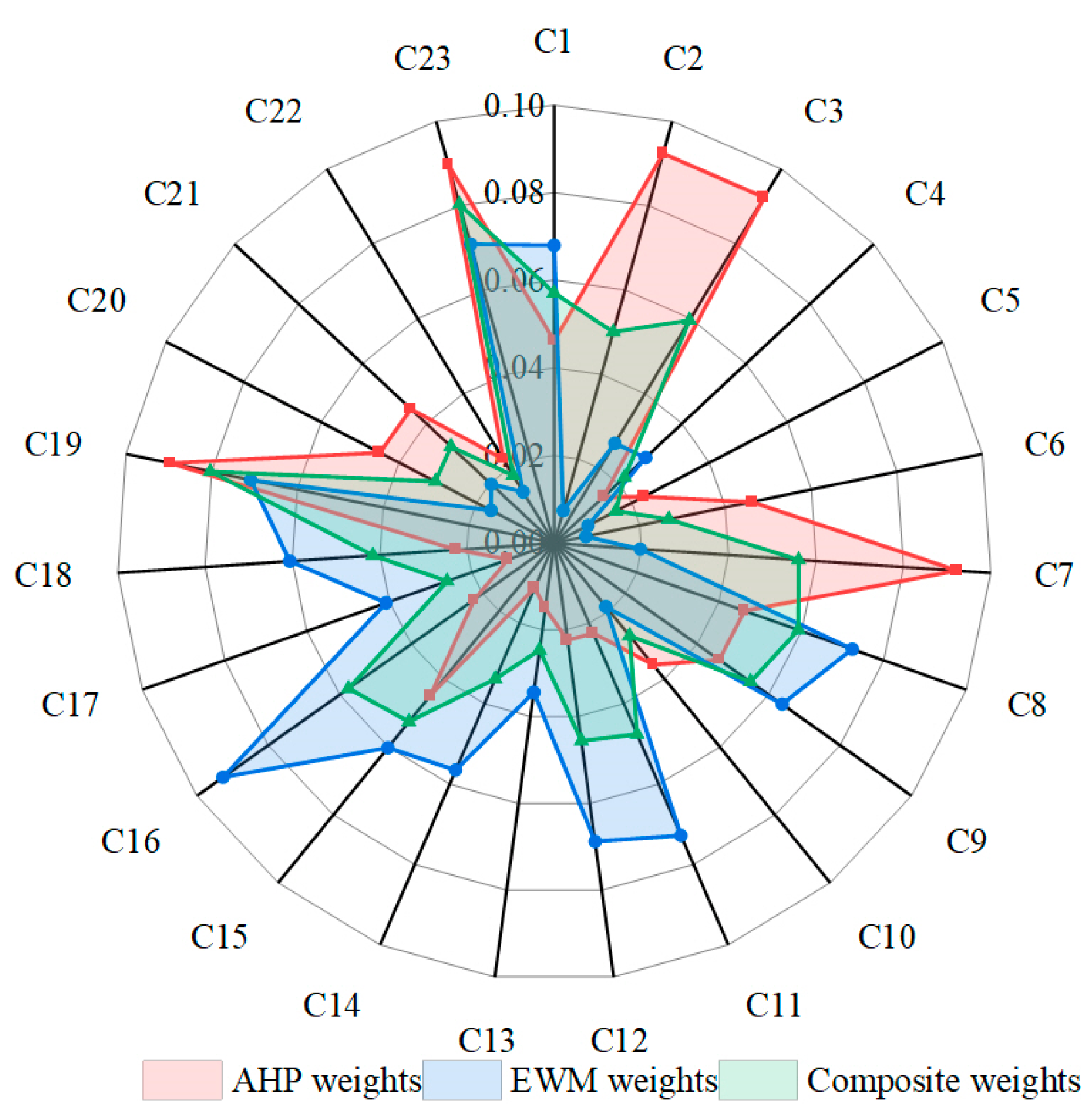
3.1. Composite Weight Results

Utilizing the AHP and the EWM, both subjective and objective weights, as well as composite weights for the three subsystem layers and nine criterion layers, encompassing a total of twenty-three evaluation indicators, were calculated. The results are presented in Figure 3. Generally, the absolute differences in weights derived from both methods were below 2% for indicators C4, C5, C9, C10, C13, C15, C19, C22, and C23. For the remaining indicators, however, the differences exceeded 2%. This disparity highlights the consistency and complementarity of the two methodologies in determining the indicator weights. When examining the subsystem layers, the weight assigned to agricultural water resource carrying capacity exceeded that of cultivated land utilization efficiency, which in turn surpassed the weight of ecological and environmental stress.

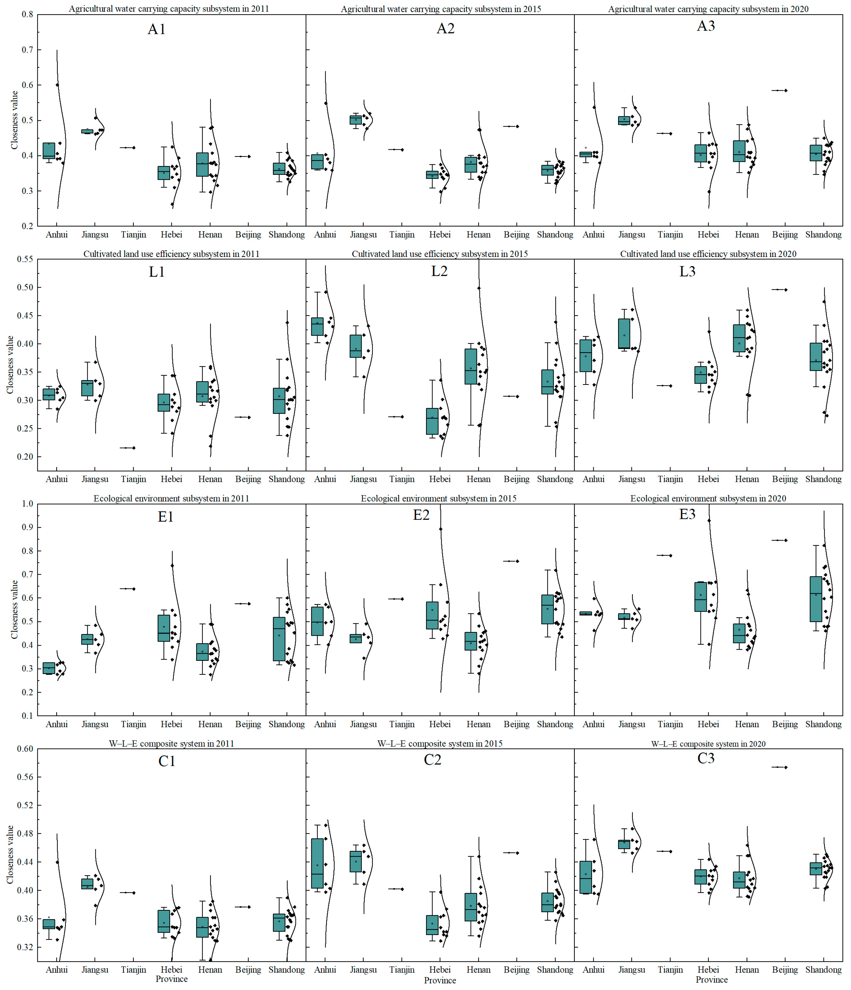
3.2. The Development Level of the W–L–E System

Based on the composite weights, the TOPSIS method was utilized to calculate the closeness of the W–L–E subsystems and the composite system to the ideal solution for the years 2011, 2015, and 2020, as shown in Figure 4. In 2011, the average index for agricultural water resource carrying capacity across seven provinces and cities was within the range of [0.351, 0.476], indicating generally weak capacity. By 2015, the index was varying slightly within [0.342, 0.501], reflecting growing regional disparities. By 2020, the index improved to [0.402, 0.585], signifying enhanced water resource capacity. The indices for cultivated land efficiency and the ecological environment exhibited a stable upward trend from 2011 to 2020. The comprehensive index for the W–L–E composite system increased significantly from [0.354, 0.405] in 2011 to [0.418, 0.574] in 2020 across the seven provinces and municipalities. The overall coefficient of variation (CV) increased from 12.65% in 2011 to 13.64% in 2015, before declining to 9.12% in 2020. This indicates a significant enhancement in the concentration of the evaluation index across the cities within each province.

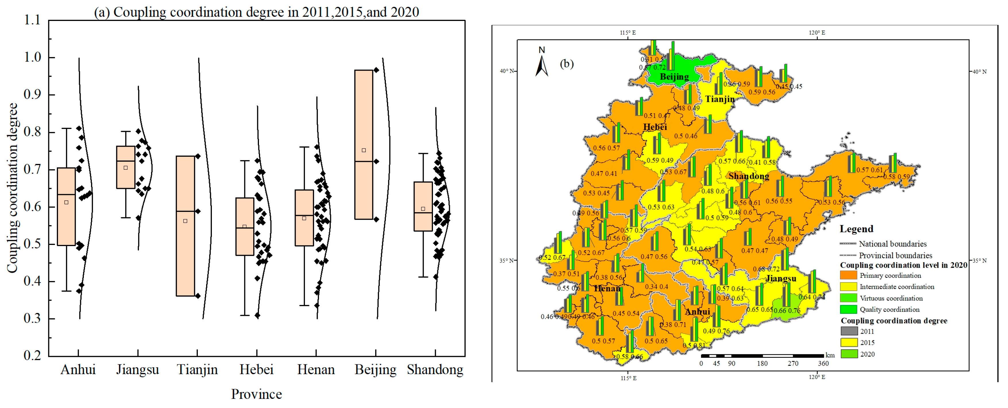
3.3. Coupling Coordination Degree of the W–L–E System

The coupling coordination degrees (CCDs) of the W–L–E system in the NCP for the years 2011, 2015, and 2020 are depicted in Figure 5. Over the decade from 2011 to 2020, the average coupling coordination levels ranked as follows: Beijing, Jiangsu, Anhui, Tianjin, Shandong, Henan, and Hebei (all seven provinces and municipalities showed improvements in their coordination indices). Specifically, Anhui, Hebei, and Henan progressed from a state of near disorder to primary coordination; Jiangsu advanced from primary to intermediate coordination; Shandong improved from a barely coordinated state to primary coordination; Beijing moved from a barely coordinated state of quality coordination (CV = 37.93%); and Tianjin significantly improved from mild disorder to intermediate coordination (CV = 42.30%). In 2020, regions with a moderate level of coordination or higher were predominantly found in Jiangsu Province, the southern part of Anhui Province, the northwestern part of Shandong Province, and the municipalities of Beijing and Tianjin.

3.4. Coupling Coordination Degree Obstacle Factors of the W–L–E System

The obstacle degree indicators of the seven provinces and municipalities were calculated for 2011, 2015, and 2020. The top 11 indicators with the highest obstacle degrees were selected as the primary obstacle factors, as shown in

Table 4. The primary obstacle factors for provinces and municipalities in 2011, 2015, and 2020.

Index	Year	Anhui	Jiangsu	Tianjin	Hebei	Henan	Beijing	Shandong	Average
C1	2011	5.82	6.11	2.86	5.40	6.98	4.26	6.52	5.42%
	2015	9.97	4.94	4.96	4.73	7.62	0.75	6.69	5.67%
	2020	9.02	5.34	3.32	4.04	7.50	0.02	5.97	5.03%
C8	2011	6.58	5.76	7.90	8.18	7.85	7.52	8.74	7.51%
	2015	9.61	7.11	7.67	9.31	8.50	8.62	9.56	8.63%
	2020	9.92	8.38	9.59	10.87	9.94	12.91	11.17	10.40%
C9	2011	6.03	5.70	7.66	7.83	6.66	6.65	6.57	6.73%
	2015	6.73	5.63	8.38	8.21	7.66	9.06	8.57	7.75%
	2020	4.91	4.91	10.70	9.85	7.58	8.14	7.48	7.65%
C11	2011	7.79	6.21	6.58	6.17	6.35	4.56	6.07	6.25%
	2015	3.02	5.22	5.50	5.31	6.04	5.36	5.24	5.10%
	2020	7.84	7.53	6.70	6.27	4.81	2.01	5.83	5.86%
C12	2011	7.57	6.95	6.70	6.24	6.58	6.88	6.68	6.80%
	2015	3.59	5.20	6.29	5.75	5.93	8.25	5.62	5.80%
	2020	7.00	5.99	7.36	6.29	5.97	13.58	5.92	7.45%
C14	2011	3.69	4.81	4.93	4.66	4.61	3.73	4.64	4.44%
	2015	6.56	6.27	5.03	4.91	5.30	4.02	5.57	5.38%
	2020	6.61	7.46	6.68	6.29	6.18	0.04	6.77	5.71%
C15	2011	4.78	4.65	8.68	5.49	4.63	9.01	5.40	6.09%
	2015	4.33	4.58	8.96	7.73	4.35	10.80	6.29	6.72%
	2020	4.30	4.60	11.00	7.11	5.18	17.06	7.22	8.07%
C16	2011	8.96	8.95	7.46	8.96	9.00	6.65	8.49	8.35%
	2015	10.22	7.95	4.90	7.70	8.08	4.53	7.45	7.26%
	2020	7.42	5.23	2.38	6.65	6.62	0.05	5.65	4.85%
C18	2011	3.77	3.68	6.87	4.33	3.66	7.12	4.27	4.81%
	2015	3.43	3.62	7.08	6.11	3.44	8.54	4.98	5.31%
	2020	3.40	3.63	8.70	5.62	4.09	13.47	5.71	6.38%
C19	2011	13.04	10.73	2.22	7.15	10.10	6.67	8.70	8.37%
	2015	11.08	12.08	3.34	7.32	11.33	2.77	7.96	7.98%
	2020	10.61	13.58	5.16	9.33	14.57	0.06	9.64	8.99%
C23	2011	7.78	6.68	12.55	10.38	10.00	6.03	9.60	9.00%
	2015	6.17	7.92	14.49	5.43	7.10	6.66	3.57	7.34%
	2020	4.14	1.72	0.98	1.00	0.67	0.00	1.09	1.37%

and Figure 6. In 2011, the primary obstacle factors included the water quality compliance rate (C23), the multiple cropping index (C19), the per capita disposable income of rural residents (C16), the water supply modulus (C8), and the per capita agricultural output value (C12). Of these, one obstacle factor relates to the water resource dimension, two to the cultivated land dimension, and two to the ecological environment dimension. In 2015, the main obstacle factors were the water supply modulus (C8), the multiple cropping index (C19), the precipitation modulus (C9), the water quality compliance rate (C23), and the per capita disposable income of rural residents (C16). Here, two factors are attributed to the water resource dimension, one to the cultivated land dimension, and two to the ecological environment dimension. In 2020, the primary obstacle factors were the water supply modulus (C8), the multiple cropping index (C19), the food security coefficient (C15), the precipitation modulus (C9), and the per capita agricultural output value (C12), all of which exhibited relatively high overall obstacle degrees. Among these, two factors belong to the water resource dimension, two to the arable land utilization benefit dimension, and one to the ecological environment dimension. During 2011 and 2015, the water quality compliance rate (C23) and per capita disposable income of rural residents (C16) were significant impeding factors within the system; however, their impact had diminished by 2020. Additionally, the water supply modulus (C8) and multiple cropping index (C19) consistently emerged as predominant constraints in 2011, 2015, and 2020.

4. Discussion

Based on the original data of the study area, composite weights were calculated using the AHP in conjunction with the entropy weight method. The TOPSIS model, the coupling coordination degree model, and the obstacle degree diagnostic model (Equations (5)–(12)) were then used to evaluate the development level, coupling coordination degree, and the key obstacle factors for each subsystem and the composite system, respectively.

4.1. Characteristics and Differences in the Closeness of the W–L–E System

The closeness to the ideal solution reflects the development levels of the subsystems and the composite system. From 2011 to 2020, the closeness value of the W–L–E composite system exhibited a fluctuating upward trend. Taking Anhui Province as an example, the closeness value was 0.362 in 2011, increased to 0.435 by 2015, but experienced a slight decline to 0.423 by 2020. In general, the closeness value in 2011 was comparatively low, indicating an overall weaker level of development. In 2015, the average closeness value increased by 9.46% compared to 2011, yet the disparities among different provinces and cities have grown. In 2020, the average closeness value further increased by 11.28% compared to 2015. This trend aligns with the research findings of Luo et al. [9]. The overall coefficient of variation (CV) for each province increased from 12.65% in 2011 to 13.64% in 2015, before declining to 9.12% in 2020. This indicates a significant enhancement in the concentration of the evaluation index across the cities within the province, reflecting a transition from asynchronous to synchronous development among various cities within each province, consistent with the research patterns reported by Lv et al. [14]. For example, in Hebei Province, the coefficient of variation (CV) was 14.06% in 2011, rising to 18.03% in 2015 and then falling to 10.43% in 2020. Over the period from 2011 to 2020, the average closeness value for the three W–L–E subsystems increased by 14.35%, 29.2%, and 34.97%, respectively, reflecting a positive trend in the development of agricultural water resource carrying capacity, cultivated land use efficiency, and ecological environment conditions in the NCP.

4.2. Coupling Coordination Condition of the W–L–E System

Due to differences in factors, such as natural endowment, location conditions, development foundations, industrial structures, and local policies, the coupling coordination of the NCP’s W–L–E system exhibits significant variation. The coupling coordination condition of the W–L–E system showed an upward trend from 2011 to 2020, increasing from 0.50 to 0.687, representing a 35.77% improvement. Over the same period, the average coupling coordination level was ranked as follows: Beijing > Jiangsu > Anhui > Tianjin > Shandong > Henan > Hebei. There was a noticeable enhancement in the average coupling coordination index for different provinces and cities. In 2020, areas with a moderate level of coordination and above accounted for 34.0%, and were mainly distributed in Jiangsu Province, the southern part of Anhui Province, the northwestern part of Shandong Province, and the municipalities of Beijing and Tianjin, reflecting distinct spatial distribution characteristics.

From 2011 to 2020, the coupling coordination degree of the three subsystems exhibited a steady growth trend, indicating a mutually reinforcing effect among the subsystems. However, there is still considerable room for improvement. This progress can be attributed to the implementation of policies such as the “National Agricultural Sustainable Development Plan (2015–2030)” and the continuous advancement of modernization projects for large and medium-sized irrigation areas following the “13th Five-Year Plan.” These efforts have led to a steady enhancement in the level of agricultural resource utilization and an increase in the coupling coordination degree values. Nevertheless, insufficient resource endowment in some regions and the extensive mode of utilization are not aligned with the pace of agricultural economic development and ecological improvements, resulting in the majority of provinces and cities being unable to achieve a highly coordinated state [50].

4.3. Diagnosis of Obstacle Factors to the W–L–E System

From a comprehensive perspective, the water quality compliance rate was a primary obstacle factor in 2011 and 2015 (ranking first and fourth, respectively), but was not a main obstacle in 2020. This shift indicates that since the “Twelfth Five-Year Plan”, ecological and environmental governance measures—including the “National Environmental Protection Plan for the Twelfth Five-Year Plan”, the “Key River Basin Water Pollution Prevention and Control Plan (2011–2015)”, the “Ecological and Environmental Protection Plan for the Thirteenth Five-Year Plan”, and the ecological protection and high-quality development strategy for the Yellow River Basin—have been effectively implemented, leading to significant improvements in the water environment conditions of the NCP. Similarly, the per capita disposable income of rural residents was a primary obstacle factor in 2011 and 2015 (ranking third and fifth, respectively), but this obstacle had significantly decreased by 2020. This improvement is closely related to policies such as “poverty alleviation and rural revitalization” [51]. The water supply modulus and multiple cropping index remained the primary obstacle factors in 2011, 2015, and 2020. On the one hand, this is due to the constraints of natural water resource endowments, with nonagricultural industries continuously encroaching on the water supply for agriculture. On the other hand, the continuous expansion of crop sowing and irrigation areas has increased agricultural water consumption, exacerbating the scarcity of water resources [3].

5. Conclusions

The development level of the W–L–E system in the seven provinces and municipalities of the NCP exhibits a fluctuating upward trend. In 2020, it ranged from 0.418 to 0.574, representing an increase of 14.6–52.3% compared to 2011. The concentration of development levels among various provinces and cities has significantly improved, with the coefficient of variation (CV) rising from 12.65% in 2011 to 13.64% and subsequently declining to 9.12% in 2020, indicating a transition from a “disordered” to an “ordered” state. Between 2011 and 2020, development levels for the W–L–E subsystems increased by 14.35%, 29.2%, and 34.97%, respectively. The coupling coordination degree of the W–L–E composite system has shown a steady growth trend from 2011 to 2020, indicating mutual promotion among the subsystems; however, there remains considerable room for improvement. In 2020, cities with an intermediate or higher degree of coordination accounted for 34.0% and were predominantly located in the southern part of Jiangsu Province, the northwestern part of Anhui Province, the northwestern part of Shandong Province, and the municipalities of Beijing and Tianjin, highlighting a distinct spatial distribution.

For the W–L–E composite system of the NCP, the obstacle factors in coupling coordination exhibited significant spatial and temporal variations. In 2011 and 2015, the water quality compliance rate and per capita disposable income of rural residents were significant obstacle factors; however, they were not primary obstacles in 2020. Additionally, the water supply modulus and multiple cropping index were the primary obstacle factors in 2011, 2015, and 2020. Furthermore, it should be noted that the subjectivity in the construction of the indicator system may introduce a degree of uncertainty to the model’s coupling results. Future research should include comparative analyses between different indicator systems and models. Meanwhile, based on the coupling coordination relationship of the W–L–E system, the optimization of the agricultural planting layout in the North China region to align with the endowment of water and soil resources should be a key focus for future studies.

6. Recommendations

Drawing on the identification results of impediments within the W–L–E system, the following policy recommendations are proposed to enhance the system’s coupling and coordination, and to foster the high-quality and harmonious development of agricultural water resources, cultivated land use, and ecological environment in the NCP:

(a)

Treat water resources as a stringent constraint, especially in regions, such as Hebei, Henan, and Shandong provinces where water supply is insufficient. Enhance the safe and efficient utilization of nonconventional water sources, including rainwater, seawater, and marginal-quality water. Advocate for localized adoption of water-saving irrigation technologies, such as integrated water-fertilizer systems, to bolster farm water supply security and irrigation efficiency through source expansion and conservation.

(b)

In accordance with the water resource carrying capacity, strictly control the total volume and intensity of agricultural water consumption across different regions. Develop water-adapted agricultural planting models, determine crop selection and production limits based on water availability.

(c)

Moderately promote the scale of agricultural operations to improve agricultural production efficiency, thereby increasing the benefits of cultivated land use and the income of agricultural workers.

(d)

Although water quality was not a primary obstacle in 2020, vigilance is necessary against the potential ecological deterioration risks associated with the expansion of crop sowing and irrigation areas, as well as the excessive use of pesticides and fertilizers.

References

1. Chiarelli, D.D.; Rosa, L.; Rulli, M.C.; D’Odorico, P. The water-land-food nexus of natural rubber production. J. Clean. Prod. 2018, 172, 1739–1747. [Google Scholar] [CrossRef]
2. Liu, X.; Xu, Y.; Sun, S.; Zhao, X.; Wang, Y. Analysis of the Coupling Characteristics of Water Resources and Food Security: The Case of Northwest China. Agriculture 2022, 12, 1114. [Google Scholar] [CrossRef]
3. Shu, J.; Bai, Y.; Chen, Q.; Weng, C.; Zhang, F. Dynamic simulation of the water-land-food nexus for the sustainable agricultural development in the North China Plain. Sci. Total Environ. 2024, 912, 168771. [Google Scholar] [CrossRef] [PubMed]
4. Li, L.; Fan, Z.; Feng, W.; Yuxin, C.; Keyu, Q. Coupling coordination degree spatial analysis and driving factor between socio-economic and eco-environment in northern China. Ecol. Indic. 2022, 135, 108555. [Google Scholar] [CrossRef]
5. Khaledian, Y.; Kiani, F.; Ebrahimi, S.; Brevik, E.C.; Aitkenhead-Peterson, J. Assessment and Monitoring of Soil Degradation during Land Use Change Using Multivariate Analysis. Land Degrad. Dev. 2016, 28, 128–141. [Google Scholar] [CrossRef]
6. Peng, J.; Pan, Y.; Liu, Y.; Zhao, H.; Wang, Y. Linking ecological degradation risk to identify ecological security patterns in a rapidly urbanizing landscape. Habitat. Int. 2018, 71, 110–124. [Google Scholar] [CrossRef]
7. Shi, J.; Wang, Z.; Zhang, Z.; Fei, Y.; Li, Y.; Zhang, F.e.; Chen, J.; Qian, Y. Assessment of deep groundwater over-exploitation in the North China Plain. Geosci. Front. 2011, 2, 593–598. [Google Scholar] [CrossRef]
8. Wang, H.; Wang, L.; Yang, G.; Jia, L.; Yao, Y.; Zhang, Y. Agricultural Water Resource in China and Strategic Measures for its Efficient Utilization. Strateg. Study CAE 2018, 20, 9–15. [Google Scholar] [CrossRef]
9. Luo, W.; Jiang, Y.; Chen, Y.; Yu, Z. Coupling Coordination and Spatial-Temporal Evolution of Water-Land-Food Nexus: A Case Study of Hebei Province at a County-Level. Land 2023, 12, 595. [Google Scholar] [CrossRef]
10. Zhang, K.; Shen, J.; He, R.; Fan, B.; Han, H. Dynamic Analysis of the Coupling Coordination Relationship between Urbanization and Water Resource Security and Its Obstacle Factor. Int. J. Environ. Res. Public Health 2019, 16, 4765. [Google Scholar] [CrossRef]
11. Zhang, Y.; Zhu, T.; Guo, H.; Yang, X. Analysis of the coupling coordination degree of the Society-Economy-Resource-Environment system in urban areas: Case study of the Jingjinji urban agglomeration, China. Ecol. Indic. 2023, 146, 109851. [Google Scholar] [CrossRef]
12. Zhang, Y.; Khan, S.U.; Swallow, B.; Liu, W.; Zhao, M. Coupling coordination analysis of China’s water resources utilization efficiency and economic development level. J. Clean. Prod. 2022, 373, 133874. [Google Scholar] [CrossRef]
13. Chen, P.; Shi, X. Dynamic evaluation of China’s ecological civilization construction based on target correlation degree and coupling coordination degree. Environ. Impact Assess. Rev. 2022, 93, 106734. [Google Scholar] [CrossRef]
14. Lv, C.; Xu, W.; Ling, M.; Wang, S.; Hu, Y. Evaluation of Synergetic Development of Water and Land Resources Based on a Coupling Coordination Degree Model. Water 2023, 15, 1491. [Google Scholar] [CrossRef]
15. Sun, B.; Tang, J.; Yu, D.; Song, Z. Coupling coordination relationship between ecosystem services and water-land resources for the Daguhe River Basin, China. PLoS ONE 2021, 16, e0257123. [Google Scholar] [CrossRef] [PubMed]
16. Li, M.; Fu, Q.; Singh, V.P.; Liu, D.; Li, T.; Zhou, Y. Managing agricultural water and land resources with tradeoff between economic, environmental, and social considerations: A multi-objective non-linear optimization model under uncertainty. Agric. Syst. 2020, 178, 102685. [Google Scholar] [CrossRef]
17. Das, B.; Singh, A.; Panda, S.N.; Yasuda, H. Optimal land and water resources allocation policies for sustainable irrigated agriculture. Land Use Policy 2015, 42, 527–537. [Google Scholar] [CrossRef]
18. Song, X.M.; Kong, F.Z.; Zhan, C.S. Assessment of Water Resources Carrying Capacity in Tianjin City of China. Water Resour. Manag. 2010, 25, 857–873. [Google Scholar] [CrossRef]
19. Tong, S.; Zhiming, F.; Yanzhao, Y.; Yumei, L.; Yanjuan, W. Research on Land Resource Carrying Capacity: Progress and Prospects. J. Resour. Ecol. 2018, 9, 331–340. [Google Scholar] [CrossRef]
20. Li, M.; Cao, X.; Liu, D.; Fu, Q.; Li, T.; Shang, R. Sustainable management of agricultural water and land resources under changing climate and socio-economic conditions: A multi-dimensional optimization approach. Agric. Water Manag. 2022, 259, 107235. [Google Scholar] [CrossRef]
21. Xie, X.; Li, X.; Fan, H. Research on the Interactive Coupling Relationship between Land Space Development and Eco-Environment from the Perspective of Symbiosis: A Practical Analysis of Henan, China. Land 2022, 11, 1252. [Google Scholar] [CrossRef]
22. He, Y.; Wang, Z. Water-land resource carrying capacity in China: Changing trends, main driving forces, and implications. J. Clean. Prod. 2022, 331, 130003. [Google Scholar] [CrossRef]
23. Pan, Y.; Ma, L.; Tang, H.; Wu, Y.; Yang, Z. Land Use Transitions under Rapid Urbanization in Chengdu-Chongqing Region: A Perspective of Coupling Water and Land Resources. Land 2021, 10, 812. [Google Scholar] [CrossRef]
24. Ma, L.; Tian, Y.; Guo, X.; Chen, M.; Wang, Y. Spatial-temporal Change of Rural Settlements and Its Spatial Coupling Relationship with Water and Soil Resources Based on Grid in the Hexi Oasis. J. Nat. Resour. 2018, 33, 775–787. [Google Scholar]
25. Ibarrola-Rivas, M.J.; Granados-Ramírez, R.; Nonhebel, S. Is the available cropland and water enough for food demand? A global perspective of the Land-Water-Food nexus. Adv. Water Resour. 2017, 110, 476–483. [Google Scholar] [CrossRef]
26. He, L.; Du, X.; Zhao, J.; Chen, H. Exploring the coupling coordination relationship of water resources, socio-economy and eco-environment in China. Sci. Total Environ. 2024, 918, 170705. [Google Scholar] [CrossRef]
27. Lin, G.; Jiang, D.; Yin, Y.; Fu, J. A carbon-neutral scenario simulation of an urban land–energy–water coupling system: A case study of Shenzhen, China. J. Clean. Prod. 2023, 383, 135534. [Google Scholar] [CrossRef]
28. Cheng, K.; He, K.; Fu, Q.; Tagawa, K.; Guo, X. Assessing the coordination of regional water and soil resources and ecological-environment system based on speed characteristics. J. Clean. Prod. 2022, 339, 130718. [Google Scholar] [CrossRef]
29. Zhu, L.; Bai, Y.; Zhang, L.; Si, W.; Wang, A.; Weng, C.; Shu, J. Water-Land-Food Nexus for Sustainable Agricultural Development in Main Grain-Producing Areas of North China Plain. Foods 2023, 12, 712. [Google Scholar] [CrossRef]
30. Liu, T.; Fang, Y.; Huang, F.; Wang, S.; Du, T.; Kang, S. Dynamic evaluation of the matching degree and utilization condition of generalized agricultural water and arable land resources in China. Trans. Chin. Soc. Agric. Eng. 2023, 39, 56–65. [Google Scholar] [CrossRef]
31. Mosleh, Z.; Salehi, M.H.; Amini Fasakhodi, A.; Jafari, A.; Mehnatkesh, A.; Esfandiarpoor Borujeni, I. Sustainable allocation of agricultural lands and water resources using suitability analysis and mathematical multi-objective programming. Geoderma 2017, 303, 52–59. [Google Scholar] [CrossRef]
32. Fan, X.; Qin, J.; Lv, M.; Jiang, M. An Evaluation System of the Modernization Level of Irrigation Districts with an Analysis of Obstacle Factors: A Case Study for North China. Agronomy 2024, 14, 538. [Google Scholar] [CrossRef]
33. Qu, B.; Jiang, E.; Li, J.; Liu, Y.; Liu, C. Coupling coordination relationship of water resources, eco-environment and socio-economy in the water-receiving area of the Lower Yellow River. Ecol. Indic. 2024, 160, 111766. [Google Scholar] [CrossRef]
34. Zhou, P.; Deng, W.; Peng, L.; Zhang, S. Spatio-temporal coupling characteristic of water-land elements and its cause in typical mountains. Acta Geogr. Sin. 2019, 74, 2273–2287. [Google Scholar] [CrossRef]
35. Yang, B.; Wang, J.; Li, S.; Huang, X. Identifying the Spatio-Temporal Change in Winter Wheat–Summer Maize Planting Structure in the North China Plain between 2001 and 2020. Agronomy 2023, 13, 2712. [Google Scholar] [CrossRef]
36. Wu, J.; Cheng, G.; Wang, N.; Shen, H.; Ma, X. Spatiotemporal Patterns of Multiscale Drought and Its Impact on Winter Wheat Yield over North China Plain. Agronomy 2022, 12, 1209. [Google Scholar] [CrossRef]
37. Mo, X.; Liu, S.; Lin, Z.; Guo, R. Regional crop yield, water consumption and water use efficiency and their responses to climate change in the North China Plain. Agric. Ecosyst. Environ. 2009, 134, 67–78. [Google Scholar] [CrossRef]
38. Yu, Z.; Deng, X. Assessment of land degradation in the North China Plain driven by food security goals. Ecol. Eng. 2022, 183, 106766. [Google Scholar] [CrossRef]
39. Zuo, Q.; Zhang, Z.; Wu, B. Evaluation of water resources carrying capacity of nine provinces in Yellow River Basin based on combined weight TOPSIS model. Water Resour. Prot. 2020, 36, 1–7. [Google Scholar] [CrossRef]
40. Ren, L.; Gao, J.; Song, S.; Li, Z.; Ni, J. Evaluation of Water Resources Carrying Capacity in Guiyang City. Water 2021, 13, 2155. [Google Scholar] [CrossRef]
41. Qin, G.; Li, H.; Wang, X.; Ding, J. Research on Water Resources Design Carrying Capacity. Water 2016, 8, 157. [Google Scholar] [CrossRef]
42. Ishizaka, A.; Labib, A. Review of the main developments in the analytic hierarchy process. Expert. Syst. Appl. 2011, 38, 14336–14345. [Google Scholar] [CrossRef]
43. Wang, Q.; Yuan, X.; Zhang, J.; Gao, Y.; Hong, J.; Zuo, J.; Liu, W. Assessment of the Sustainable Development Capacity with the Entropy Weight Coefficient Method. Sustainability 2015, 7, 13542–13563. [Google Scholar] [CrossRef]
44. Ma, J.; Fan, Z.; Huang, L. A subjective and objective integrated approach to determine attribute weights. Eur. J. Oper. Res. 1999, 112, 397–404. [Google Scholar] [CrossRef]
45. Hwang, C.; Kwangsun, Y. Multiple Attribute Decision Making—Methods and Applications: A State-of-the-Art Survey; Springer: New York, NY, USA, 1981. [Google Scholar]
46. Lei, X.; Robin, Q.; Liu, Y. Evaluation of regional land use performance based on entropy TOPSIS model and diagnosis of its obstacle factors. Trans. Chin. Soc. Agric. Eng. 2016, 32, 243–253. [Google Scholar] [CrossRef]
47. Çelikbilek, Y.; Tüysüz, F. An in-depth review of theory of the TOPSIS method: An experimental analysis. J. Manag. Anal. 2020, 7, 281–300. [Google Scholar] [CrossRef]
48. Zhao, Y.; Shi, H.; Miao, Q.; Yang, S.; Hu, Z.; Hou, C.; Yu, C.; Yan, Y. Analysis of Spatial and Temporal Variability and Coupling Relationship of Soil Water and Salt in Cultivated and Wasteland at Branch Canal Scale in the Hetao Irrigation District. Agronomy 2023, 13, 2367. [Google Scholar] [CrossRef]
49. Chen, Y.; Zhu, M.; Lu, J.; Zhou, Q.; Ma, W. Evaluation of ecological city and analysis of obstacle factors under the background of high-quality development: Taking cities in the Yellow River Basin as examples. Ecol. Indic. 2020, 118, 106771. [Google Scholar] [CrossRef]
50. Zhang, J.; Dong, Z. Assessment of coupling coordination degree and water resources carrying capacity of Hebei Province (China) based on WRESP2D2P framework and GTWR approach. Sustain. Cities Soc. 2022, 82, 103862. [Google Scholar] [CrossRef]
51. Qin, M.; Wu, G.; Liu, J. A Coupling and Coordination Analysis of Agricultural Water Resources Carrying Capacity and Cultivated Land Use Efficiency. J. Nat. Sci. Hunan Norm. Univ. 2023, 46, 97–105. [Google Scholar]
Figure 1. Location of the North China Plain within China.
Agriculture 14 01636 g001
Figure 2. The flowchart of the study methodology.
Agriculture 14 01636 g002
Figure 3. The weights of the evaluation indicators.
Agriculture 14 01636 g003
Figure 4. The evaluation indices of agricultural water resources subsystem (W1–W3), cultivated land subsystem (L1–L3), s ecological environment subsystem (E1–E3), and W–L–E composite system (C1–C3) in 2011, 2015, and 2020. Note: The study, which is based on municipal-level data, indicates that there are fewer data points for Beijing and Tianjin.
Agriculture 14 01636 g004
Figure 5. Coupling coordination degree of the W–L–E system in 2011, 2015, and 2020, where (a) is the overall graph and (b) is the city-specific graph.
Agriculture 14 01636 g005
Figure 6. Coupling coordination degree obstacle factors in 2011, 2015, and 2020.
Agriculture 14 01636 g006