Abstract
The centrifuge method serves as an efficient and rapid approach for determining the soil–water characteristic curve (SWCC). However, soil shrinkage during centrifugation remains overlooked and prior modified methods may suffer from complex operations, high costs, time consumption, and limited applicability. To address these issues, this study introduces a simple correction scheme (G3) for determining drying SWCCs using the centrifuge method based on high matric suction calibration points. The performance of the proposed G3 method was systematically evaluated against a modified method considering soil shrinkage (G1) and the conventional uncorrected method (G2). Results revealed significant soil linear shrinkage post-centrifugation, accompanied by a reduction in total soil porosity and an increase in soil bulk density. SWCCs from all methods exhibited strong consistency at low matric suction ranges but diverged markedly at high matric suction segments. High matric suction data dominated the SWCC fitting. The G1 method achieved the highest fitting accuracy, while the G3 method performed the worst yet maintained acceptable reliability. The G2 method yielded optimal SWCC for simulating saturated soil water content, field capacity, and permanent wilting point. Conversely, Hydrus-1D simulations revealed superior performance of the G3 method in simulating farmland soil moisture dynamics during the dehumidification process. Values of R2 across methods followed G3 > G1 > G2, while mean absolute error, mean absolute percentage error, and root mean square error exhibited the opposite trend. These findings highlight that the previous modified approaches are more suitable for low and medium matric suction ranges. The proposed correction method enhances drying SWCC performance across the full matric suction range, offering a practical refinement for the centrifuge method. This advancement could enhance the reliability in soil hydraulic characterization and contribute to a better understanding of the hydraulic–mechanical–chemical behavior in soils.
1. Introduction
Soil water serves as the linchpin of the water cycle and ecohydrological processes in the terrestrial surface system [1]. Understanding the mechanisms of soil water retention and movement holds significant scientific value. The soil–water characteristic curve (SWCC), which illustrates the relationship between the quantity (content or saturation) and energy (matric suction) of soil water, represents one of the most crucial hydraulic properties of soil [2]. Fundamentally, the SWCC offers insights into both the hydraulic parameters and pore size distribution of soil [3,4,5]. Furthermore, it is indispensable for simulating soil water evaporation, infiltration, distribution, and solute transport [6,7,8]. Obviously, precise determination of the SWCC is critical in research fields such as hydrology, geology, and agricultural engineering.
The laboratory SWCC determination methods mainly include the filter paper method, pressure plate method, centrifuge method, chilled mirror method, and vapor equilibrium method [4,9,10,11]. The pressure plate method is a traditional way for determining SWCC, which uses the axis-translation technique to control soil matric suction [12,13]. However, this method is typically labor-intensive and time-consuming (often requiring weeks or months). Recently, the centrifuge method has gained widespread use because it overcomes these shortcomings and offers an extensive matric suction measurement range with dependable outcomes [4,14]. Several researchers have employed the centrifuge method to determine SWCCs and pedotransfer functions (PTFs) for diverse soil types [4,15,16], or to examine the hydraulic properties of soil and their influencing factors [17,18,19]. However, soil gradually shrinks during centrifugation, changing the bulk density (BD), pore structure, and hydraulic properties of soil, especially under a high matric suction range [4,6,10]. Previous research has shown that the BD of loam soils increased from an initial value of 1.30 g cm−3 to 1.57–1.72 g cm−3 after centrifugation [20]. Such variations induce deviations in the soil volumetric water content, making it impossible to establish the relationship between centrifugal force (soil matric suction) and soil saturation [6,11,21]. Meanwhile, due to the combined effect of supergravity and matric suction during soil shrinkage, the SWCC measured by the centrifuge method differs from that measured by the pressure plate method, although their consistency is good [14,22].
In recent years, several beneficial attempts have been made to modify the centrifuge method. Fu et al. [10] and Li et al. [4] proposed methods to restrict soil shrinkage during centrifugation and effectively eliminate their impacts on SWCCs. Some scholars have proposed combining the centrifuge method (at low matric suction ranges) with the chilled mirror method (at high matric suction ranges), with results showing good agreement with SWCCs measured by the pressure plate method [9,23]. However, despite their effectiveness, these methods often involve complex operational procedures or require additional equipment and high costs. Xing et al. [6] and Lai et al. [21] suggested correcting observed data based on soil shrinkage characteristics during centrifugation to obtain the optimal SWCC. Whether simulating cumulative soil infiltration based on SWCCs or inverting soil hydraulic parameters from infiltration data, the employment of a calibrated SWCC offers more precise outcomes, as soil shrinkage during dehydration occurs concurrently with matric suction changes [2,24]. However, Xing et al. [6] and Lai et al. [21] did not consider observed data in a high matric suction range when determining SWCCs; additionally, this method may cause certain model parameters to exceed their thresholds, thereby limiting the applicability of this approach (see Section 2.4).
Regrettably, we identified at least 20 studies (Table S1) in the past 5 years that have overlooked the effect of soil shrinkage when using the centrifuge method to determine SWCC under the assumption of constant BD. Although the centrifuge method serves as an effective supplement to the pressure plate method, its limitations have not received sufficient attention, potentially introducing uncertainties in related research areas. Meanwhile, existing modified schemes for centrifuge methods suffer from complex operational procedures, labor-intensive processes, time-consuming workflows, high costs, and limited applicability. To address these issues, this study proposes a simple approach to calibrate an SWCC that retains the centrifuge method framework. The core principle involves taking observed raw data from the high matric suction segment (≥1500 kPa) that does not consider the impacts of soil shrinkage as calibration points to correct SWCCs (see Section 2.4). The main purpose of this study is to (a) investigate the impacts of soil shrinkage and BD variations on SWCCs derived from the centrifuge method and (b) develop a simple SWCC correcting method using high matric suction calibration points and assess its performance through simulations of soil water constants and farmland soil moisture dynamics (via Hydrus-1D model).
2. Materials and Methods
2.1. Soil Sampling
Soil samples were collected from the Shouyang Dryland Agroecosystems National Field Scientific Observatory and Research Station (37°45′ N, 113°12′ E, 1202 m a.s.l., Figure 1). This station is located in Shouyang County, Shanxi Province, at the eastern edge of the Loess Plateau, and exhibits a warm-temperate continental semi-humid climate. The average annual temperature at the station is approximately 8.2 °C, and the average annual precipitation is approximately 481 mm. Five adjacent typical newly reclaimed farmlands (10 m × 10 m) were selected as sample plots (numbered S1–S5), and a test pit with a depth of 60 cm was excavated at the center of each plot. The test pit depth was defined by the vertical extent of the soil zone subject to rapid moisture fluctuation. At each pit, in situ soils were collected to determine the SWCC at depths of 10, 20, 30, 40, and 60 cm using a specific cutting ring, with 2 replicates at each depth. A total of three independent samplings were conducted in June 2022, February 2023, and September 2023. In total, accounting for variations across plots, soil depths, and sampling times, 150 soil samples were obtained for determining SWCCs. In addition, a total of 225 disturbed or in situ soil samples were collected synchronously next to the SWCC sampling sites for determining individual indicators of the soil physical properties, water constants and saturated hydraulic conductivity, with three replicates per depth.
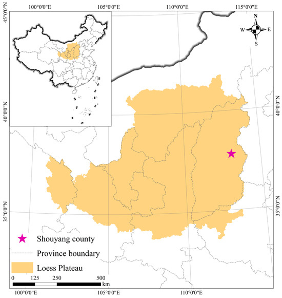
Figure 1.
Location of the experimental site in Shanxi Province, China.
2.2. Determination of the Soil Physical Properties, Water Constants, and Saturated Hydraulic Conductivity
The BD and soil particle density (PD) were determined using the cutting ring method and pycnometer test method, respectively, and the total soil porosity (TP) was calculated according to the BD and PD [25,26] (Table S2). The soil texture was determined using a Mastersizer 2000 (Malvern Panalytical, Ltd., Malvern, UK) and classified as sand (0.05–2 mm), loam (0.002–0.05 mm), and clay (0–0.002 mm) according to United States Department of Agriculture (USDA) standards [27]. The textures of the selected soil samples were loam, sandy loam, and silty loam, as shown in Figure 2.
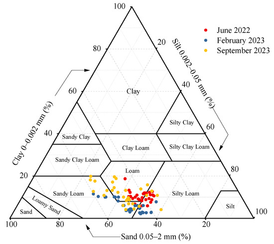
Figure 2.
Soil textures of selected samples classified by the United States Department of Agriculture standards across three independent samplings.
The soil water constants included the saturated soil water content (θs), field capacity (FC) and permanent wilting point (PWP) (Table S2). Using the cutting ring method and Wilcox method, the θs and FC were determined, respectively, and then both of them were represented as volumetric water content. The determination of the PWP is difficult and time-consuming, so the PTF established by the gene expression programming method [28] was employed to estimate the values. This PTF was developed from 192 soil samples with different textures, including loam, sandy loam, and silty loam. The equation (coefficient of determination equal to 0.873) can be expressed as follows:
where BD is the soil bulk density (g cm−3), silt and clay denote the fractions of silt and clay in the soil, respectively (%), and dg is the geometric particle size diameter (mm), which can be calculated according to the method of Shirazi and Boersma [29].
The saturated soil hydraulic conductivity (Ks, Table S2) was measured using the constant-head method (via Mariotte Bottle) and then converted to the standard value at 10 °C [30].
2.3. Establishment of the SWCC
2.3.1. Operation Process of the Centrifuge Method
The SWCC was determined using a CR21G II high-speed refrigerated centrifuge (Hitachi, Ltd., Tokyo, Japan) at 20 °C. The in situ soil samples were saturated with distilled water for 24 h and then placed in a rotor (R11D2) together with matching containers (for details, refer to Kong et al. [19]) after weighing. Centrifugation was conducted sequentially at different revolution speeds (Table 1), and the samples were removed at the corresponding equilibrium times. Then, the mass (mi, in g, where i denotes the i-th centrifugation step, the same hereafter) and surface sedimentation (Δzi, cm) of the soil samples were determined using an electronic balance (Shimadzu, Ltd., Kyoto, Japan) and digital vernier calipers, with three repetitions. Finally, the soil samples were dried in an oven at 105 °C until a constant weight was reached, then the mass (md, g) was measured three times.

Table 1.
Revolution speeds and equilibrium time for each centrifugation step.
2.3.2. Calculation of the Soil Matric Suction and Volumetric Water Content
The soil matric suction can be calculated based on the revolution speed and corresponding centrifugal radius as follows [31]:
where hi is the soil matric suction at the i-th centrifugation step (cm), ω is the angular velocity (rad s−1), ρ is the pure water density (1 g cm−3), g is the gravitational acceleration (980 cm s−1), R1 is the radial distance to the mid-point of the soil samples (cm), which varies with Δzi, and R2 is the radial distance to the bottom of the soil samples (cm).
Obviously, if soil shrinkage is not considered (Δzi ≡ 0), then R1 is a constant. Hence, the soil matric suction calculated by Equation (2) is only related to the revolution speeds, denoted as hi’.
Soil samples shrink along both the radial and axial directions during centrifugation. However, the magnitude of radial shrinkage is minimal and can be disregarded [10,21]. Therefore, it is proposed that the soil volume changes throughout centrifugation can be exclusively attributed to axial shrinkage, and the BD at the different revolution speeds can be calculated based on Δzi as follows:
where γdi is the BD at the i-th centrifugation step (g cm−3), H is the initial height of the soil sample (equal to 5 cm), V is the volume of the cutting ring (equal to 100 cm3), and δi (equal to Δzi divide H) is the soil axial linear shrinkage ratio at the i-th centrifugation step. The other symbols have the same meaning as before.
The soil volumetric water content can be calculated by the soil weight water content and BD:
where θi is the soil volumetric moisture content at the i-th centrifugation step (cm3 cm−3). The other symbols have the same meaning as before.
Obviously, if soil shrinkage is not considered (Δzi ≡ 0), the BD calculated by Equation (3) will remain constant during centrifugation and will always match the initial value (i.e., γd0). Accordingly, the soil volumetric moisture content calculated by Equation (4) can be labeled as θi′.
2.3.3. Fitting Model of the SWCC
Numerous empirical and theoretical models have been developed to describe the SWCC, such as the Brooks–Corey model [32], the Gardner model [33], the van Genuchten model [34], and the Fredlund and Xing model [35]. The van Genuchten (VG) model is particularly prevalent owing to its simplicity, superior fitting accuracy, extensive applicability across soil textures and matric suction ranges, and the closed-form expression for predicting the hydraulic conductivity of unsaturated soils [2,36]. The VG model can be expressed as follows:
where θs is the saturated volumetric water content (cm3 cm−3), θr is the residual volumetric water content (cm3 cm−3), α (cm−1) is the inverse of the air-entry value (AEV), n and m are parameters that describe the shape of the SWCC (m = 1 − 1/n), θ and h are the measured soil volumetric water content (cm3 cm−3) and matric suction (cm), respectively, used to establish the SWCC.
The well-established computer code RETC (version 6.02) was employed to fit the SWCC via a nonlinear least-squares optimization technique [37]. Subsequently, by substituting h-values of 0, 33, and 1500 kPa (i.e., 0 cm, 336 cm, and 15,296 cm) into the VG model, the corresponding soil water contents were calculated as θs, FC, and PWP, respectively [28].
2.4. Correcting of the SWCC
A typical unimodal SWCC exhibits an S-shape when plotted in semilogarithmic coordinates and can generally be divided into three segments: low, medium, and high soil matric suction ranges. The dry end refers to the part where θ spans from PWP to the oven-dried soil water content, typically corresponding to the high matric suction segment of SWCCs [38,39]. A study covering multi-soil types further demonstrated that the average soil saturation at the boundary between the medium and high matric suction segments is 0.29 [36], closely aligning with the PWP range in this study. Consequently, we define the matric suction exceeding 1500 kPa (equal to 15,296 cm) as the high soil matric suction segment of SWCCs.
van Genuchten [34] defined θr as the value of θ at which dθ/dh approaches zero in the high matric suction segment of SWCCs, thereby simplifying soil water retention behavior in specific ranges [35,40] and leading to suboptimal performance at the dry end of SWCCs [16,41,42]. Evidently, considering the soil shrinkage and BD changes exacerbates this issue. If θr exceeds measured soil water content, it fails to reflect true soil hydraulic properties in the numerical simulations [43,44]. Notably, the maximum soil matric suction in experiments conducted by Xing et al. [6] and Lai et al. [21] did not exceed 1000 kPa (equal to 10,194 cm), potentially limiting the applicability of the correction method. The matric suction range of measurement data is critical for obtaining optimal SWCCs and the VG model is highly sensitive to this range [8]. SWCCs derived from limited data (without high matric suction ranges) remain unreliable even with high coefficients of determination [36], resulting in overestimated soil water content [44,45,46,47]. While previous studies indicate that calibrated SWCCs (considering the soil shrinkage and BD changes) improve simulations of soil moisture movement and hydraulic parameter inversion [6,21], this approach may only be valid for low to medium matric suction ranges, with questionable reliability in high matric suction segment.
This study therefore proposes a modified centrifuge approach that is simple, rapid, and reliable for obtaining the optimal SWCC. Firstly, increase the maximum revolution speed of the centrifuge to extend measurement data into the high matric suction segment of SWCCs (soil matric suction exceeding 1500 kPa). Secondly, incorporate soil shrinkage and BD changes to correct measurement data in low to medium matric suction ranges, as described in Section 2.3.2 and supported by Xing et al. [6] and Lai et al. [21]. Thirdly, the raw observation data of soil water content and matric suction (without accounting for soil shrinkage) in the high suction segment are used as calibration points to adjust and thereby enhance the dry-end performance of SWCCs. This approach combines corrected low to medium matric suction observed data (θi, hi) with uncorrected high matric suction raw data (θi’, hi’) for SWCC fitting. Crucially, this method operates entirely within the original centrifuge method framework without extra equipment or procedures.
Finally, this study evaluated three SWCC determination methods based on the centrifuge technique: G1. correcting SWCC by accounting for soil shrinkage and BD changes (θi, hi); G2. uncorrected SWCC neglecting soil shrinkage (θi’, hi’); G3. correcting SWCC via high matric suction calibration points. Furthermore, it is critical to emphasize that the evaluation of SWCC fitting methods must incorporate the applicability of high matric suction ranges.
2.5. Simulations of Farmland Soil Moisture Dynamics via the Hydrus-1D Model
The Hydrus-1D model, developed by the U.S. Salinity Laboratory, was designed to simulate water, heat, and solute movement in one-dimensional variably saturated soil. The program is user-friendly, feature-rich, and offers flexible boundary conditions, rendering it a reliable tool for simulating soil water dynamics under both field and laboratory conditions [48,49]. The Hydrus-1D program aims to numerically solve the Richards equation for water flow in variably saturated soil [50], which can be expressed as follows:
where θ is the soil volumetric water content (cm3 cm−3), t is the time (d), h is the soil matric suction (cm), z is the vertical space coordinate (cm), S(z, t) is the source–sink term (cm d−1), namely, the root water uptake rate, and K(h) is the soil hydraulic conductivity at any h (cm d−1).
K(h) can be calculated via the Mualem model [51] as follows:
where Ks is the saturated soil hydraulic conductivity (cm d−1), Se is the effective saturation (cm3 cm−3), and l is the pore connectivity parameter (equal to 0.5). The meanings of the other symbols are the same as before.
In the Hydrus-1D model, S(z, t) can be calculated using the drought stress response function proposed by Feddes et al. [52]:
where α(h, z) is the water stress response function, b(z) is a normalized function describing the distribution of the root length density, and Tp is the potential crop transpiration rate (cm d−1).
2.5.1. Setting of the Initial and Boundary Conditions for the Hydrus-1D Model
During the periods from June to November 2022 and from April to September 2023, deficit irrigation experiments were conducted on the sample plots to establish distinct soil water gradients. The tested crop was greenhouse tomato irrigated via surface drip irrigation. To minimize potential adverse effects of crop root growth and SWCC hysteresis on model accuracy, the typical soil dehumidification process at the tomato maturity stage were simulated. The specific simulation periods included the following: September 1st to 7th (M1), September 10th to 19th (M2), and September 28th to October 9th (M3) in 2022; and August 20th to 27th (M4), August 29th to September 4th (M5), and September 6th to 13th (M6) in 2023.
The simulated soil profile depth was 60 cm (61 nodes in total), stratified into five layers according to soil properties, namely, 0–10 cm, 10–20 cm, 20–30 cm, 30–40 cm, and 40–60 cm. Observation points were set at 10 cm intervals (nodes 6, 16, 26, 36, 46, and 56 in the soil profile). Given the absence of irrigation during the specific simulation periods (M1–M6), coupled with the soil surface being covered by plastic film and the groundwater table occurring deep below, the surface boundary condition was configured as a zero flux boundary, and the bottom boundary condition was configured as a free drainage boundary. Initial model conditions were determined by soil volumetric water content measured at each simulation start using Shang detector (Insentek Co., Ltd., Hangzhou, China) installed at the center of each plot. These devices monitored real-time soil moisture dynamics across 0–60 cm depth (with an interval of 10 cm). In addition, the Hydrus-1D model employed a fixed 1 day time step for simulations.
2.5.2. Setting of the Hydrus-1D Model Parameters
The parameter Ks was measured directly (Table S2), while θs, θr, α, and n were derived from VG models fitted using different methods. Notably, these parameters for the simulations in 2022 (M1–M3) and 2023 (M4–M6) were calculated from soil samples collected in February and September 2023, respectively.
The parameter b(z) was determined based on crop root length density. Post-harvest, multi-point samples of tomato roots were collected at 10 cm intervals to 60 cm depth using a root auger (Zhejiang Top Yunnong Technology Co., Ltd., Hangzhou, China) in October 2022 and September 2023, respectively. Sampling was repeated three times per plot. Root samples were soaked in water and manually washed through sieves. Then, dead and miscellaneous material were removed filtered by color and shape. Root length density (Table S3) was quantified with a Performance V800 photo scanner (Epson Co., Ltd., Suwa, Japan) and WinRHIZO Pro2009 root analysis software (Regent Instruments Inc., Quebec City, QC, Canada). The parameter Tp depends on crop reference evapotranspiration (ET0), crop coefficient (Kc), leaf area index (LAI), and extinction coefficient (β) [53]. During simulations, ET0–calculated via the modified Penman–Monteith equation [54] using greenhouse microclimate data exhibited minor variation (Figure S1), and Kc, LAI, and β were also treated as constants. Thus, Tp was assumed to remain consistent throughout each simulation period [55].
With parameters b(z) and Tp held constant, and no severe or prolonged water stress observed in tomato plants during simulation periods (α(h, z) = 1), root water uptake rate (S(z, t)) was considered constant in this study. Moreover, entirely plastic mulch coverage further allowed neglect of soil evaporation, equating root water uptake rate to crop daily water consumption intensity [56]. Accordingly, α(h, z) = 1 and Tp was set as the average daily crop water consumption intensity in this study (Table S4), enabling the simulation of daily root water uptake rate by the Feddes model. Daily crop water consumption intensity can be determined using the water balance equation excluding rainfall, irrigation, groundwater recharge, runoff, and deep drainage [57].
2.6. Data Analysis and Model Evaluation
Data analysis was conducted using Excel 2016 (Microsoft Corporation, Redmond, WA, USA) and SPSS Statistics 20.0 (IBM Electronics, Armonk, NY, USA), while plotting was performed with Origin 2024 (OriginLab Corporation, Northampton, MA, USA). Duncan’s new multiple range test was employed for single-factor analysis of variance to ascertain whether there was a significant difference (p < 0.05). A two-tailed t test was utilized to determine the statistical significance of Pearson’s correlation coefficient (r, p < 0.05). The fitting accuracy of the model was assessed using the coefficient of determination (R2), mean absolute error (MAE), mean absolute percentage error (MAPE), and root mean square error (RMSE), which were calculated according to the method of Xing et al. [2]. The closer the R2 value is to 1 or the lower the MAE, MAPE, and RMSE values are, the better the model simulation effect.
where Si denotes the simulated value, Oi denotes the measured value, k is the total number of observations, and denotes the average value of Oi.
3. Results
3.1. Soil Shrinkage and BD Changes During Centrifugation
With increasing revolution speed, soil matric suction gradually increased, while soil sample height decreased to varying extents (Figure 3a). Across three experiments, the maximum measured matric suction reached 18,360 cm (September 2023), with an average peak value of 16,277 cm. The soil axial linear shrinkage ratio (δ) also peaked at maximum revolution speed, reaching mean values of 23.7% (June 2022), 18.9% (February 2023), and 16.8% (September 2023), respectively. The magnitude of the soil axial linear shrinkage ratio followed June 2022 > February 2023 > September 2023. The trends of matric suction were the opposite. Furthermore, a significant negative correlation existed between soil axial linear shrinkage ratio and matric suction (p < 0.001) at fixed revolution speeds.
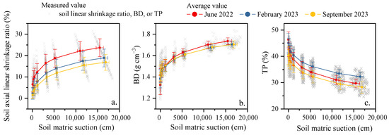
Figure 3.
Variations in (a) soil axial linear shrinkage ratio, (b) bulk density (BD) and (c) total porosity (TP) under different matric suctions during centrifugation across three independent samplings.
The soil samples compacted during centrifugation, leading to an increase in BD. However, the extent of increasement decreased with rising matric suction (Figure 3b). The average BD values were 1.74 g cm−3 in June 2022, 1.70 g cm−3 in February 2023, and 1.70 g cm−3 in September 2023 post-centrifugation. Compared to the initial values (1.33, 1.38, and 1.42 g cm−3, respectively), there was a significant increase of 30.9%, 23.2%, and 20.2%, respectively (p < 0.001). However, TP declined with increasing matric suction (Figure 3c). Post-centrifugation, the mean TP decreased significantly (p < 0.001) from 46.4% in June 2022, 45.0% in February 2023, and 40.4% in September 2023 before centrifugation to 29.8%, 32.3%, and 28.3% (35.8%, 28.3%, and 29.9% reductions), respectively. Overall, the mean TPs across all revolution speeds are ranked as follows: February 2023 > June 2022 > September 2023.
Correlation analysis (Figure 4) demonstrated that soil axial linear shrinkage ratio was significantly positively correlated with BD (r = 0.6281, p < 0.001) and significantly negatively correlated with TP (r = −0.5381, p < 0.001). Concurrently, initial TP exhibited a significant negative correlation with maximum BD (r = −0.2316, p = 0.04) and a substantial positive correlation with the increase in BD (r = 0.4553, p < 0.001). This indicates that soils with higher initial TP are more compaction-prone.
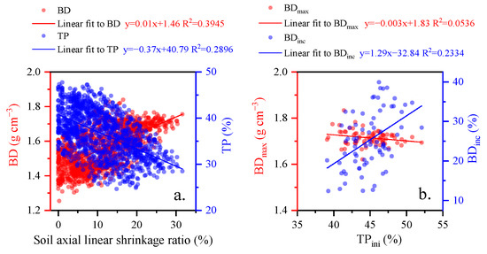
Figure 4.
Correlations between (a) soil axial linear shrinkage ratio with both bulk density (BD) and total porosity (TP), and (b) initial TP (TPini) with both maximum BD (BDmax) and BD increase rate (BDinc) post-centrifugation.
3.2. Comparison of SWCCs Derived from Different Methods
In this study, 75 SWCCs were constructed for five soil depths, three sampling replicates and five trial plots. Results showed that the VG model demonstrated favorable fitting performance across various conditions and methods (Figure 5). Under the G1, G2, and G3 methods, the median R2 values of the VG models were 0.9950, 0.9944, and 0.9803; the median MAE values were 0.0046, 0.0059, and 0.0108 cm3 cm−3; the median MAPE values were 2.01%, 2.78%, and 5.05%; and the median RMSE values were 0.0048, 0.0065, and 0.0096 cm3 cm−3, respectively. Although differences were minor, the G1 method (considering soil shrinkage and BD changes) slightly improved the fitting accuracy of SWCC compared to the uncorrected model (G2). Meanwhile, the G3 method exhibited relatively poor accuracy due to the use of fitting data from two distinct datasets. However, SWCCs calibrated via raw data in the high soil matric suction segment remained reliable (R2 ≥ 0.9615, MAE ≤ 0.0148 cm3 cm−3, MAPE ≤ 6.86%, and RMSE ≤ 0.0133 cm3 cm−3).
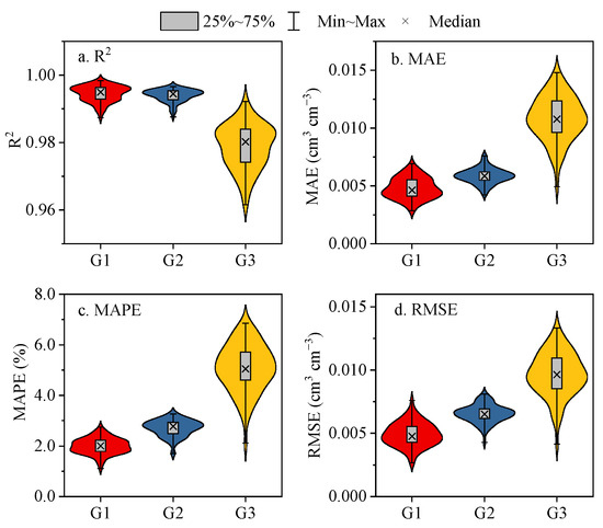
Figure 5.
Performance metrics of the VG model: (a) R2, (b) MAE, (c) MAPE, and (d) RMSE values across different methos and samplings. Note: R2 represents the coefficient of determination; MAE represents mean absolute error; MAPE represents mean absolute percentage error; and RMSE represents root mean square error.
Figure 6 shows SWCCs derived from different methods using soil samples collected in September 2023, with one soil layer depth per plot as a representative case. The results indicated that whether considering soil shrinkage and BD changes (G1) or not (G2), the shapes and positions of SWCCs in the low matric suction segment were nearly identical. However, compared to the G2 method, SWCCs under the G1 method were elevated and exhibited reduced curvature in the medium to high matric suction ranges. For identical matric suctions, the corresponding soil volumetric water content under the G1 method was notably higher, attributable to BD increases caused by soil shrinkage during centrifugation. SWCCs calibrated via raw data in the high matric suction segment (G3) aligned more closely with the curves obtained from the G2 method, though only the calibration points data fully matched. Overall, SWCCs derived from the G3 method were flatter, with lower soil volumetric water content at both extreme low and high matric suction ranges (h > 108 cm). Furthermore, beyond a certain matric suction threshold, differences between SWCCs remained constant.
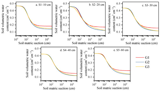
Figure 6.
Schematic diagram of soil–water characteristic curves across different methods with one soil depth for each plot ((a) S1–10 cm, (b) S2–20 cm, (c) S3–30 cm, (d) S4–40 cm, and (e) S5–60 cm) in September 2023.
The variations in VG model parameters highlighted differences between SWCCs derived from different methods. θs maintained nearly identical values across all three methods (p = 1.000; Figure 7a). Conversely, θr was significantly higher (p < 0.001) under the G1 method (mean value of 0.1659 cm3 cm−3) compared to the G2 method (mean value of 0.1080 cm3 cm−3), with a median increase of 51.2%. This indicates that accounting for soil shrinkage and BD changes overestimates θr (Figure 7b). After correcting SWCCs with high matric suction calibration points, the values of θr became zero in 20% of SWCCs. Therefore, the G3 method yielded a significantly lower θr (mean value of 0.0739 cm3 cm−3) with 55.4% and 31.6% reductions (p < 0.001) compared to the G1 and G2 methods, respectively. In contrast, α under the G3 method (mean value of 0.0235 cm−1; Figure 7c) notably increased (p < 0.001) by 63.4% and 53.7%, respectively, relative to the G1 (mean value of 0.0144 cm−1) and G2 (mean value of 0.0153 cm−1) methods. In addition, the value of α differed by less than 10% between the G1 and G2 methods. Finally, values of the curve-shape factor n consistently followed G1 > G2 > G3 (Figure 7d). The G1 method produced a mean n of 1.46, significantly higher (p < 0.01) than the G2 (mean value of 1.36) and G3 (mean value of 1.25) methods, corresponding to increases of 7.73% and 17.2%, respectively.
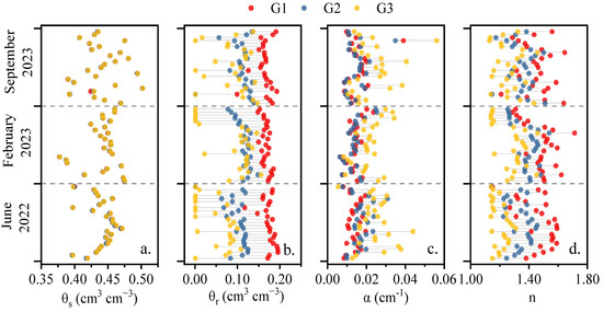
Figure 7.
The parameters of the VG model: (a) saturated volumetric water content (θs), (b) residual volumetric water content (θr), (c) inverse of the air-entry value (α), and (d) curve-shape factor (n) across different methods and samplings.
3.3. Evaluation of SWCCs Based on Simulations of Soil Water Constants and Farmland Soil Moisture Dynamics
Soil water constants (θs, FC and PWP) estimated by SWCCs were compared with measured data (Figure 8). Results indicated that the G3 method was slightly more accurate than the other methods in simulating θs, despite minimal observed differences (Table 2). However, both FC (mean value of 0.2547 cm3 cm−3) and PWP (mean value of 0.1143 cm3 cm−3) were generally overestimated, particularly PWP. Under the G1, G2, and G3 methods, the mean values of simulated FC were 0.2997, 0.2938, and 0.3040 cm3 cm−3, respectively, with MAPE of 18.23%, 16.20%, and 19.93%, respectively; the mean values of simulated PWP were 0.1947, 0.1626, and 0.1776 cm3 cm−3, respectively, with MAPE of 70.52%, 42.37%, and 55.48%, respectively. The VG model exhibited the highest fitting accuracy for FC and PWP simulations under the G2 method. These findings demonstrated that soil shrinkage and BD changes should be ignored when constructing SWCCs using the centrifuge method, from the perspective of producing relatively accurate soil water constants.
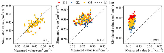
Figure 8.
Measured and simulated values of soil water constants: (a) saturated volumetric water content (θs), (b) field capacity (FC) and (c) permanent wilting point (PWP) across different methods and samplings.
Table 2.
Accuracy of simulated soil water constants across different methods and samplings.
The farmland soil moisture dynamics within the root zone (0–60 cm depth) during the dehumidification process at the tomato maturity stage were simulated via the Hydrus-1D model (Figure 9). Despite variations in soil hydraulic parameters (θs, θr, α and n) across different methods, the Hydrus-1D model yielded reasonably accurate results. Under the G1, G2, and G3 methods, the simulated mean soil water contents in 2022 were 0.2095, 0.2091, and 0.2093 cm3 cm−3, respectively, with an average measured value of 0.2142 cm3 cm−3; in 2023, the simulated mean values were 0.1855, 0.1823, and 0.1826 cm3 cm−3, respectively, with an average measured value of 0.1896 cm3 cm−3. Overall, all methods significantly underestimated soil water content (p < 0.01). Sample plot S4 serves as an example to illustrate soil moisture dynamics and simulation outcomes under various soil depths and periods in 2022 (M1–M3; Figure S2). The Hydrus-1D model exhibited higher accuracy in simulating shallow soil moisture dynamics (0–30 cm depth). No consistent patterns were observed in simulated soil moisture dynamics or model accuracy across methods at the different soil depths.
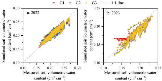
Figure 9.
Measured and simulated soil volumetric water content during typical dehumidification at tomato maturity stage across different methods in year (a) 2022 (M1–M3) and (b) 2023 (M4–M6). Note: Simulation periods were set as September 1st to 7th (M1), September 10th to 19th (M2), and September 28th to October 9th (M3) in 2022; and August 20th to 27th (M4), August 29th to September 4th (M5), and September 6th to 13th (M6) in 2023.
However, the simulations showed higher accuracy and more pronounced inter-method differences in 2022 (Table 3). For both the single dataset and aggregated data, the MAE, MAPE, and RMSE of the models followed the pattern of G3 < G1 < G2, while R2 exhibited the opposite trend. This suggests that utilizing soil hydraulic parameters incorporating soil shrinkage and BD changes (G1) improves ability of the Hydrus-1D model to capture soil water dynamics during dehumidification. Further accuracy gains were achieved by correcting SWCCs with high matric suction calibration points (G3). Furthermore, data from plots S1 and S3 in 2023 were excluded. Since θr exceeded initial soil water content at certain depths under G1 method, the prevented model execution was prevented. These results demonstrate that the high matric suction calibration points are essential for optimizing SWCC determined by the centrifuge method in soil moisture dynamics simulations.
Table 3.
Accuracy of simulated soil volumetric water content during typical dehumidification at tomato maturity stage across different methods in year 2022 (M1–M3) and 2023 (M4–M6).
4. Discussion
4.1. Soil Shrinkage and BD Changes During Centrifugation Cannot Be Neglected
Soil is a loose and porous medium composed of solid, liquid, and gas phase substances. Normally, soil particles and liquids are not compressible, meaning soil volumetric changes reflect the pore structure alterations on a macroscopic view. Studies demonstrate that under centrifugal force, as soil pore water drains, primary pores (macropores and mesopores) undergo a large-scale collapse, forcing soil particle rearrangement until compressive deformation peaks [4,6,11]. This study observed significant axial-dominant soil shrinkage during centrifugation (Figure 3a). Meanwhile, the soil axial linear shrinkage ratio showed a strong negative correlation with TP (Figure 4a), confirming soil pore structure modification. In addition, the magnitude of soil shrinkage also correlated with soil texture. Soils collected in 2023 generally had higher sand content and exhibited smaller axial linear shrinkage ratios than those taken in 2022 (Figure 2). This is consistent with the previous study [58]. Notably, soil radial shrinkage remained negligible despite minor surface cracking, consistent with our hypothesis and reports in other studies [4,10,21]. However, Xing et al. [2] reported that soil exhibits comparable axial–radial shrinkage post-centrifugation, generating a large number of soil surface cracks. These cracks may enhance the soil hydraulic conductivity [59], thereby further amplifying uncertainties in SWCCs derived from the centrifuge method.
Soil shrinkage resulted in BD increases (Figure 3b). The soils analyzed in this study exhibited loam, sandy loam, and silty loam textures, with BD increases of 10.0–46.2%, 12.0–43.5%, and 10.0–33.6% post-centrifugation, respectively. This indicates that heavier-textured and finer-grained soils are more susceptible to disturbance by centrifugal force. Similarly, loamy and powdery loam soils showed BD increases of 20.8–32.3% [20] and 28.3–47.3% [6], respectively, at the end of centrifugation, whereas sandy loam soil exhibited only 7.1–26.2% BD increase [4]. Meanwhile, we found that BD increases across soil textures were significantly positively correlated with initial TP of soil, while post-centrifugation maximum BD converged to similar values (mean value of 1.71 g cm−3; Figure 4b). Thus, soils with lower initial BD, loose structure, and well-developed pores experienced greater shrinkage yet attained smaller final BD values after centrifugation. Crucially, soil shrinkage and BD changes during centrifugation differ from drying shrinkage or mechanical compaction due to synergistic supergravity and matric suction effects [11,60]. The alterations in soil pore structure during centrifugation could be further analyzed via scanning electron microscopy or mercury intrusion porosimetry, but this falls beyond the scope of this study.
4.2. Impacts of Soil Shrinkage and BD Changes on the SWCC
The soil shrinkage and BD changes were not obvious under the low revolution speeds (Figure 3); therefore, the SWCCs derived from different methods highly overlapped in the low matric suction ranges, and the values of θs were almost identical (Figure 6 and Figure 7). This is consistent with the reports of other scholars [6,20,41], indicating that soil shrinkage and BD changes exert a minimal influence on θs.
The air-entry value (AEV, equivalent to 1/α) is governed by the radius of the largest soil pores [4]. The larger the pore size, the easier it is for air to expel water from soil pores. During centrifugation, the geometric dimensions of dominant pores decrease with the collapse of macropores and mesopores, causing soils to retain saturation at elevated matric suction and increasing AEV. Consequently, when accounting for soil shrinkage and BD changes (G1), the value of α (the inverse of AEV) decreased (Figure 7). Similar results have been reported for sandy loam, loam, and calcic vertisol soils [6,41]. However, SWCC correction via high matric suction calibration points (G3) overestimated α, contradicting actual soil structural changes during centrifugation. The value of AEV does not alter the shape of SWCCs but shifts its position along the matric suction axis [46]. Therefore, the critical points of the SWCC under the G3 model typically corresponded to a lower matric suction.
Variations in SWCCs across methods primarily manifested in shape differences, particularly within the high matric suction segment. When soil shrinkage and BD changes were considered (G1), SWCC tails shifted upward with flattened curvature, and θr was greatly overestimated (Figure 6 and Figure 7). This is consistent with prior findings [4,6,21]. This phenomenon directly stems from the significant BD increases under high matric suction (Figure 3) and fundamentally reflects how pore structure plays a dominant role in soil hydraulic properties. For a specific soil, the factors influencing SWCCs primarily act through pore structure modifications, where minor changes can drastically alter soil hydraulic behavior [24,40,61]. Progressive soil compression reduces volumes of macropores and mesopores, increases micropore proportion, and diminishes pore connectivity, forming denser and homogeneous pore structure that hinder pore water drainage [20,62,63]. Hence, shrinking soils exhibit enhanced water-holding capacity, reduced water-releasing capacity, and lower SWCC curvature compared to undisturbed soils (Figure 5). Conversely, the G3 method underestimated θr. Furthermore, SWCCs derived from the G3 method generally fell between the other two methods and closely resembled the uncorrected curve (G2) within the range of θ spans from PWP to oven-dried soil water content (h = 107 cm). This confirms that the measurement data in the high matric suction segment dominate the SWCC fitting. The VG model has the most sensitivity to the matric suction range of observed data [8]; therefore, omitting dry-end data leads to the SWCC systematic overestimation of soil water content [44,45,46,47]. It proves high matric suction calibration points are both effective and necessary for optimizing SWCC dry-end performance.
The parameter n governs the slope of the transition zone (between AEV and θr) of SWCCs [46]. Consistent with Xing et al. [6] and Chen et al. [41], this study revealed that n was overestimated when soil shrinkage and BD changes were accounted for (Figure 7). However, Li et al. [20] and Wen et al. [24] reached the opposite conclusion. It has been reported that n is an increasing function of the SWCC slope [51]. With other VG model parameters kept constant, a higher n results in a steeper SWCC [46]. This contradicts the findings of this study. We found that n values across methods could be roughly ordered as G1 > G2 > G3; however, the SWCC under the G2 method was obviously steeper (Figure 7). This suggests that n depends not only on soil physical properties (e.g., pore structure) but also on the fitted models, observed data, and other model parameter values.
4.3. Optimizing SWCCs Derived from the Centrifuge Method via High Matric Suction Calibration Points
This study revealed that the VG model exhibited excellent fitting accuracy across all methods. Moreover, the performance of SWCCs could be further enhanced by accounting for soil shrinkage and BD changes (G1), as shown in Figure 5. These findings align with reports from other scholars. Chen et al. [41] noted that when soil shrinkage was considered, R2 of the VG model increased from 0.789–0.922 to 0.904–0.950, while RMSE decreased from 0.022–0.034 cm3 cm−3 to 0.018–0.025 cm3 cm−3. Saha and Sekharan [64] examined natural soils with varying plastic limits and found that considering soil shrinkage generally increased R2 of the VG model. In contrast, correcting SWCCs via high matric suction calibration points (G3) resulted in poorer fitting accuracy. This is unsurprising, as the G3 method combined corrected low to medium matric suction data (considering soil shrinkage and BD changes) with uncorrected high matric suction data (calibration points). Nevertheless, SWCCs derived from the G3 method were still reliable and accurate.
From the perspective of modeling soil water constants, uncorrected SWCCs (G2) demonstrated the highest accuracy (Figure 8 and Table 2). Meanwhile, correcting SWCCs via high matric suction calibration points (G3) substantially improved dry-end performance compared to the G1 method. However, no method could yield accurate values of soil water constants except θs, particularly PWP, which was severely overestimated. This aligns with the reports of Shang and Li [16] and Angelaki et al. [65]. There are three potential explanations. First, the fixed θr in the VG model oversimplifies the soil water retention behavior at high matric suction ranges, compromising the dry-end performance of SWCCs [35,40,41,42]. Second, SWCCs fitted with limited data (excluded high matric suction segment) deviate from actual curves, thereby overestimating soil water content [44,45,46,47]. Third, PWP estimates relied on PTF in this study, which may lack applicability in local areas, despite with robust dataset foundations. Thus, the superiority of SWCC determining methods cannot be determined solely through soil water constant simulations. Additionally, we recommend that the VG model should not be used for PWP estimation unless full matric suction range data are available.
The Hydrus-1D model was employed to simulate farmland soil moisture dynamics during dehumidification (Figure 9 and Figure S2), with method performances evaluated accordingly (Table 3). Results showed that accounting for soil shrinkage and BD changes (G1) enhanced model simulation accuracy, while further improvements were achieved through correcting SWCCs via high matric suction calibration (G3). Soil hydraulic conductivity (both saturated and unsaturated) critically controls vadose zone water movement, with unsaturated conductivity playing a dominant role [30,66,67,68]. As stated in Section 2.5, soil saturated hydraulic conductivity (Ks) was consistent across methods (Table S2), implying that improved soil moisture dynamics simulations stem from accurate unsaturated hydraulic conductivity estimation due to optimization of SWCC parameters. It should be noted that this study did not investigate the soil hydraulic conductivity function (HCF), i.e., the relationship between soil hydraulic conductivity and matric suction (or water content or degree of saturation). Like the SWCCs, the HCFs exhibit highly nonlinear characteristics and are governed by soil pore structure [69]. Previous studies indicate that soil shrinkage during centrifugation promotes soil crack formation, significantly enhancing hydraulic conductivity of unsaturated soil [2,59]. Neglecting soil shrinkage may cause unsaturated hydraulic conductivity estimated based on the VG model to deviate by 102 to 104 orders of magnitude [64]. Similarly, Lai et al. [21] found shrinkage-corrected SWCC better matched the curves obtained through inversion based on one-dimensional soil infiltration tests. These findings underscore the necessity of incorporating soil shrinkage and BD changes in SWCCs derived from the centrifuge method, aligning with the soil dry shrinkage behavior.
Notably, measured soil water content generally decreased from near FC to a level close to θr during the simulation periods (Figure 7 and Figure 9), spanning medium to high matric suction ranges. The actual soil water content in 2023 (mean value of 0.1896 cm3 cm−3) was lower than that in 2022 (mean value of 0.2141 cm3 cm−3), indicating higher matric suction. However, the Hydrus-1D model exhibited lower accuracy under the G1 method in 2023 (Table 3). This confirms limited applicability of prior SWCC correction methods in the high matric suction range. By contrast, correcting SWCCs via high matric suction calibration points (G3) improved both soil moisture simulations and dry-end performance, validating its efficacy for centrifuge method optimization. However, it is crucial to emphasize that this study did not account for the potential effects of SWCC hysteresis. Driven by the ink-bottle effect, aging phenomena, entrapped air effects, the contact angle difference, and capillary condensation, the soil water content at a given matric suction is generally higher during the drying process than the wetting process [9,70,71]. Hysteresis significantly influences soil hydraulic and mechanical behavior as well as microbial activity, resulting in distinct SWCCs, HCFs, and shear strength functions (SSFs) for unsaturated soils between drying and wetting cycles [72,73]. Appropriate soil hydraulic properties should be selected based on the actual process the soil undergoes (i.e., drying or wetting) [9]. Consequently, the findings of this study are valid specifically for the soil drying process, and the proposed modified method is applicable for determining drying SWCCs.
Finally, the assumption of constant root water uptake ratio (equating actual daily crop water consumption intensity; Section 2.5) in a given simulation period diverges from the real conditions. Additionally, studies suggest soil hydraulic parameters measured under steady-state conditions may inadequately characterize the transient water movement in farmlands [74,75]. These factors potentially compromise Hydrus-1D performance. Meanwhile, data from plots S1 and S3 in 2023 were excluded from modeling due to θr exceeding initial soil water content under the G1 method, which prevented model execution. Model overfitting occasionally occurred, transforming θr into empirical correction factors that mask physical characteristics of parameter, thereby failing to reflect true soil hydraulic properties and amplifying model uncertainty [43,44]. Critically, correcting SWCCs via high matric suction calibration points (G3) avoids the limitation in this study.
5. Conclusions
To address the impacts of soil shrinkage and limitations of prior modified schemes in SWCCs derived from the centrifuge method, this study proposes a simple method (G3) via high matric suction calibration points to correct drying SWCCs. The key findings are as follows: (1) Significant soil shrinkage occurred post-centrifugation (mean linear axial shrinkage ratio of 16.8–23.7%), accompanied by altered pore structures (28.3–35.8% reduction in average TP) and increased mean BD (20.2–30.9%). (2) SWCCs across all methods diverged at high matric suction range. The G1 method (accounting for soil shrinkage and BD changes) generated upward-tailing SWCCs with reduced curvature, elevated θr and n values, and underestimated α, primarily driven by pore structure changes. SWCCs derived from the G3 method resembled the uncorrected curves (G2), indicating high matric suction data dominance in SWCC fitting. (3) The G1 method achieved the highest SWCC fitting accuracy, while the G3 method performed the worst, yet maintained acceptable reliability. (4) For simulating soil water constants (θs, FC, and PWP), the G2 method demonstrated superior accuracy. However, Hydrus-1D simulations revealed optimal farmland soil moisture dynamics accuracy under the G3 method (MAE, MAPE, and RMSE: G3 < G1 < G2; R2 inversely ranked). This enhancement stems from improved soil unsaturated hydraulic conductivity estimation via optimization of SWCC parameters. This study confirms the necessity of considering soil shrinkage and BD changes in determining SWCCs via the centrifuge method. The proposed method via high matric suction calibration points effectively enhances drying SWCC performance across full matric suction ranges, offering a practical refinement for centrifuge-based determinations. This advancement could enhance the reliability in soil hydraulic characterization, thereby helping to advance our knowledge of the hydraulic–mechanical–chemical behavior in soils. Notably, the conclusions are valid specifically for the soil drying process and determining drying SWCCs.
Supplementary Materials
The following supporting information can be downloaded at https://www.mdpi.com/article/10.3390/agriculture15212223/s1, Figure S1: Reference evapotranspiration (ET0) for greenhouse tomatoes during simulation periods in year (a) 2022 (M1–M3) and (b) 2023 (M4–M6); Figure S2: Measured and simulated soil volumetric water dynamic in plot S4 during typical dehumidification in year 2022 (M1-M3) across different methods and soil depths; Table S1: Summary of recent studies omitting soil shrinkage in centrifuge-based SWCC determination; Table S2: Basic physical properties (BD, PD, and TP) and saturated hydraulic conductivity (Ks) of soil at different depths across sample plots; Table S3: Root length density of tomato at maturity stage across soil depths and sample plots; Table S4: Potential crop transpiration rate (Tp, cm d−1) for simulation periods in all sample plots.
Author Contributions
Conceptualization, B.L.; methodology, B.L.; formal analysis, B.L.; investigation, B.L. and H.P.; data curation, B.L., H.P. and Y.T.; writing—original draft preparation, B.L.; writing—review and editing, X.J.; supervision, X.J.; project administration, B.L.; funding acquisition, B.L. All authors have read and agreed to the published version of the manuscript.
Funding
This research was funded by the National Natural Science Foundation of China (Grant No. 52209062), the Fundamental Research Program of Shanxi Province (Grant No. 202103021223144), the Young Science & Technology Leadership Program (Grant No. 2023YQPYGC08), the Shanxi Province Excellent Doctor Award Fund (Grant No. SXBYKY2022061), and the Science and Technology Innovation Fund of Shanxi Agricultural University (Grant No. 2021BQ95).
Institutional Review Board Statement
Not applicable.
Data Availability Statement
The original contributions presented in this study are included in the article/Supplementary Material. Further inquiries can be directed to the corresponding author.
Acknowledgments
Authors thank grateful to the editors and reviewers for their insightful comments and suggestions.
Conflicts of Interest
The authors declare no conflicts of interest.
References
- Sprenger, M.; Tetzlaff, D.; Buttle, J.; Carey, S.K.; Mcnamara, J.P.; Laudon, H.; Shatilla, N.J.; Soulsby, C. Storage, mixing, and fluxes of water in the critical zone across northern environments inferred by stable isotopes of soil water. Hydrol. Process 2018, 32, 1720–1737. [Google Scholar] [CrossRef]
- Xing, X.; Kang, D.G.; Ma, X. Differences in loam water retention and shrinkage behavior: Effects of various types and concentrations of salt ions. Soil Tillage Res. 2017, 167, 61–72. [Google Scholar] [CrossRef]
- Rattan, B.; Dwivedi, M.; Garg, A.; Sekharan, S.; Sahoo, L. Combined influence of water-absorbing polymer and vegetation on soil water characteristic curve under field condition. Plant Soil 2024, 499, 491–502. [Google Scholar] [CrossRef]
- Li, L.; Li, X.; Wang, L.; Hong, B.; Shi, J.; Sun, J. The effects of soil shrinkage during centrifuge tests on SWCC and soil microstructure measurements. B Eng. Geol. Environ. 2020, 79, 3879–3895. [Google Scholar] [CrossRef]
- Wu, H.; Lei, X.W.; Chen, X.; Shen, J.H.; Wang, X.Z.; Ma, T.T. Study on Effect of Particle Size Distribution on Water-Retention Capacity of Coral Sand from Macro and Micro Perspective. J. Mar. Sci. Eng. 2024, 12, 341. [Google Scholar] [CrossRef]
- Xing, X.; Li, Y.; Ma, X. Water retention curve correction using changes in bulk density during data collection. Eng. Geol. 2018, 233, 231–237. [Google Scholar] [CrossRef]
- Zhou, H.; Zhao, W.Z. Modeling soil water balance and irrigation strategies in a flood-irrigated wheat-maize rotation system. A case in dry climate, China. Agr. Water Manag. 2019, 221, 286–302. [Google Scholar] [CrossRef]
- Rahimi, A.; Rahardjo, H.; Leong, E.C. Effect of range of soil-water characteristic curve measurements on estimation of permeability function. Eng. Geol. 2015, 185, 96–104. [Google Scholar] [CrossRef]
- Ma, J.; Zeng, R.; Bian, S.; Meng, X.; Zhang, Z.; Khalid, Z. Prediction of hysteretic soil and water characteristic curve of loess based on multifractal theory and improved physical statistics. J. Hydrol. 2024, 632, 130898. [Google Scholar] [CrossRef]
- Fu, X.; Shao, M.; Lu, D.; Wang, H. Soil water characteristic curve measurement without bulk density changes and its implications in the estimation of soil hydraulic properties. Geoderma 2011, 167–168, 1–8. [Google Scholar] [CrossRef]
- Rao, J.; Yi, L.; Wan, Y.; Wen, T.; Chen, Z. Dual effects of supergravity deformation and suction deformation on the determination of soil water characteristic curve by centrifugal testing method. Soil Tillage Res. 2025, 249, 106495. [Google Scholar] [CrossRef]
- Liu, H.; Rahardjo, H.; Satyanaga, A.; Du, H. Use of osmotic tensiometers in the determination of soil-water characteristic curves. Eng. Geol. 2023, 312, 106938. [Google Scholar] [CrossRef]
- Hamdany, A.H.; Shen, Y.; Satyanaga, A.; Rahardjo, H.; Lee, T.D.; Nong, X. Field instrumentation for real-time measurement of soil-water characteristic curve. Int. Soil Water Conserv. Res. 2022, 10, 586–596. [Google Scholar] [CrossRef]
- Reatto, A.; Da Silva, E.M.; Bruand, A.; Martins, E.S.; Lima, J.E.F.W. Validity of the Centrifuge Method for Determining the Water Retention Properties of Tropical Soils. Soil Sci. Soc. Am. J. 2008, 72, 1547–1553. [Google Scholar] [CrossRef]
- Wang, Y.; Zhang, A.; Ren, W.; Niu, L. Study on the soil water characteristic curve and its fitting model of Ili loess with high level of soluble salts. J. Hydrol. 2019, 578, 124067. [Google Scholar] [CrossRef]
- Shang, L.; Li, D. Comparison of different approaches for estimating soil water characteristic curves from saturation to oven dryness. J. Hydrol. 2019, 577, 123971. [Google Scholar] [CrossRef]
- Jia, A.; Song, X.; Li, S.; Liu, Z.; Liu, X.; Han, Z.; Gao, H.; Gao, Q.; Zha, Y.; Liu, Y.; et al. Biochar enhances soil hydrological function by improving the pore structure of saline soil. Agr. Water Manag. 2024, 306, 109170. [Google Scholar] [CrossRef]
- Chen, J.; Wu, Z.; Zhao, T.; Yang, H.; Long, Q.; He, Y. Rotation crop root performance and its effect on soil hydraulic properties in a clayey Utisol. Soil Tillage Res. 2021, 213, 105136. [Google Scholar] [CrossRef]
- Kong, D.; Wu, T.; Xu, H.; Jiang, P.; Zhou, A.; Lv, Y. Variation and correlation between water retention capacity and gas permeability of compacted loess overburden during wetting-drying cycles. Environ. Res. 2024, 252, 118895. [Google Scholar] [CrossRef] [PubMed]
- Li, L.; Li, X.; Lei, H.; Hong, B.; Wang, L.; Zheng, H. On the characterization of the shrinkage behavior and soil-water retention curves of four soils using centrifugation and their relation to the soil structure. Arab. J. Geosci. 2020, 13, 1259. [Google Scholar] [CrossRef]
- Lai, Y.; Garg, A.; Chang, K.; Xing, X.; Fan, J.; Liang, J.; Yu, M. A novel method to inverse the water retention curves with consideration of volume change during centrifuge testing. Soil Sci. Soc. Am. J. 2021, 85, 207–216. [Google Scholar] [CrossRef]
- Bittelli, M.; Flury, M. Errors in Water Retention Curves Determined with Pressure Plates. Soil Sci. Soc. Am. J. 2009, 73, 1453–1460. [Google Scholar] [CrossRef]
- Rahardjo, H.; Nong, X.F.; Lee, D.T.T.; Leong, E.C.; Fong, Y.K. Expedited Soil–Water Characteristic Curve Tests Using Combined Centrifuge and Chilled Mirror Techniques. Geotech. Test. J. 2017, 41, 207–217. [Google Scholar] [CrossRef]
- Wen, T.; Chen, X.; Shao, L. Effect of multiple wetting and drying cycles on the macropore structure of granite residual soil. J. Hydrol. 2022, 614, 128583. [Google Scholar] [CrossRef]
- Federico, A.M.; Miccoli, D.; Murianni, A.; Vitone, C. An indirect determination of the specific gravity of soil solids. Eng. Geol. 2018, 239, 22–26. [Google Scholar] [CrossRef]
- Robinson, D.A.; Thomas, A.; Reinsch, S.; Lebron, I.; Feeney, C.J.; Maskell, L.C.; Wood, C.M.; Seaton, F.M.; Emmett, B.A.; Cosby, B.J. Analytical modelling of soil porosity and bulk density across the soil organic matter and land-use continuum. Sci. Rep. UK 2022, 12, 7085. [Google Scholar] [CrossRef]
- Corral-Pazos-De-Provens, E.; Rapp-Arrarás, Í.; Domingo-Santos, J.M. Estimating textural fractions of the USDA using those of the International System: A quantile approach. Geoderma 2022, 416, 115783. [Google Scholar] [CrossRef]
- Shiri, J.; Keshavarzi, A.; Kisi, O.; Karimi, S. Using soil easily measured parameters for estimating soil water capacity: Soft computing approaches. Comput. Electron. Agr. 2017, 141, 327–339. [Google Scholar] [CrossRef]
- Shirazi, M.A.; Boersma, L. A Unifying Quantitative Analysis of Soil Texture. Soil Sci. Soc. Am. J. 1984, 48, 142–147. [Google Scholar] [CrossRef]
- Tan, S.; Su, X.; Jiang, X.; Yao, W.; Chen, S.; Yang, Q.; Ning, S. Irrigation Salinity Affects Water Infiltration and Hydraulic Parameters of Red Soil. Agronomy 2023, 13, 2627. [Google Scholar] [CrossRef]
- Gardner, W.R. A method of measuring the capillary tension of soil moisture over a wide moisture range. Soil Sci. 1937, 4, 277–284. [Google Scholar] [CrossRef]
- Brooks, R.H.; Corey, A.T. Hydraulic Properties of Porous Media. Hydrol. Pap. 1964, 7, 26–28. [Google Scholar]
- Gardner, W.R. Some steady-state solutions of the unsaturated moisture flow equation with application to evaporation from a water table. Soil Sci. 1958, 85, 228–232. [Google Scholar] [CrossRef]
- van Genuchten, M.T. A closed-form equation for predicting the hydraulic conductivity of unsaturated soils. Soil Sci. Soc. Am. J. 1980, 44, 892–898. [Google Scholar] [CrossRef]
- Fredlund, D.G.; Xing, A. Equations for the soil-water characteristic curve. Can. Geotech. J. 1994, 31, 521–532. [Google Scholar] [CrossRef]
- Ren, X.; Kang, J.; Ren, J.; Chen, X.; Zhang, M. A method for estimating soil water characteristic curve with limited experimental data. Geoderma 2020, 360, 114013. [Google Scholar] [CrossRef]
- Van Genuchten, M.T.; Leij, F.J.; Yates, S.R. The RETC Code for Quantifying the Hydraulic Functions of Unsaturated Soils; U.S. Environmental Protection Agency: Washington, DC, USA, 1991. [Google Scholar]
- Liao, K.; Lai, X.; Zhou, Z.; Zhu, Q.; Han, Q. A simple and improved model for describing soil hydraulic properties from saturation to oven dryness. Vadose Zone J. 2018, 17, 180082. [Google Scholar] [CrossRef]
- Du, C. A novel segmental model to describe the complete soil water retention curve from saturation to oven dryness. J. Hydrol. 2020, 584, 124649. [Google Scholar] [CrossRef]
- Hou, X.; Qi, S.; Li, Y.; Liu, F.; Li, T.; Li, H. Hydraulic conductivity over a wide suction range of loess with different dry densities. J. Rock Mech. Geotech. Eng. 2024, 17, 418–492. [Google Scholar] [CrossRef]
- Chen, Y.M.; Guo, Z.C.; Gao, L.; Qian, Y.Q.; Zhang, Z.B.; Peng, X.H. Description and modeling of the impacts of rigid calcareous concretions and shrinkage on the water retention curve of a Vertisol. Soil Tillage Res. 2024, 239, 106039. [Google Scholar] [CrossRef]
- Khlosi, M.; Cornelis, W.M.; Douaik, A.; van Genuchten, M.T.; Gabriels, D. Performance evaluation of models that describe the soil water retention curve between saturation and oven dryness. Vadose Zone J. 2008, 7, 87–96. [Google Scholar] [CrossRef]
- Zhai, Q.; Rahardjo, H.; Satyanaga, A. Effects of residual suction and residual water content on the estimation of permeability function. Geoderma 2017, 303, 165–177. [Google Scholar] [CrossRef]
- Fang, Q.; Ren, X.; Zhang, B.; Chen, X.; Guo, Z. A flexible soil-water characteristic curve model considering physical constraints of parameters. Eng. Geol. 2022, 305, 106717. [Google Scholar] [CrossRef]
- Zhou, J.; Ren, J.; Li, Z. An improved prediction method of soil-water characteristic curve by geometrical derivation and empirical equation. Math. Probl. Eng. 2021, 1, 9956824. [Google Scholar] [CrossRef]
- Rastgou, M.; He, Y.; Wang, J.; Bayat, H.; Shao, M.; Li, Y.; Jiang, Q. A technical evaluation on the mathematical attitudes and fitting accuracy of soil moisture retention curve models. Comput. Electron. Agr. 2023, 215, 108347. [Google Scholar] [CrossRef]
- Uzundurukan, S. Predictive models for the residual saturation zone of the soil–water characteristic curve. J. Soil. Sediment. 2023, 23, 3974–3989. [Google Scholar] [CrossRef]
- Aimůnek, J.; van Genuchten, M.T.; Aejna, M. Recent developments and applications of the HYDRUS computer software packages. Vadose Zone J. 2016, 15, 2014–2016. [Google Scholar] [CrossRef]
- Kumar, H.; Srivastava, P.; Lamba, J.; Diamantopoulos, E.; Ortiz, B.; Morata, G.; Takhellambam, B.; Bondesan, L. Site-specific irrigation scheduling using one-layer soil hydraulic properties and inverse modeling. Agr. Water Manag. 2022, 273, 107877. [Google Scholar] [CrossRef]
- Richards, L.A. Capillary conduction of liquids through porous mediums. J. Appl. Phys. 1931, 5, 318–333. [Google Scholar] [CrossRef]
- Mualem, Y. A new model for predicting the hydraulic conductivity of unsaturated porous media. Water Resour. Res. 1976, 12, 513–522. [Google Scholar] [CrossRef]
- Feddes, R.A.V.; Kowalik, P.J.; Zaradny, H. Simulation of Field Water Use and Crop Yield; Wageningen Centre for Agricultural Publishing and Documentation: Wageningen, The Netherlands, 1978. [Google Scholar]
- Wenzel, J.L.; Pöhlitz, J.; Usman, M.; Piernicke, T.; Conrad, C. Enhancing irrigation scheduling by application efficiency estimations and soil moisture simulations. Eur. J. Agron. 2025, 164, 127487. [Google Scholar] [CrossRef]
- Fernández, M.D.; Bonachela, S.; Orgaz, F.; Thompson, R.; López, J.C.; Granados, M.R.; Gallardo, M.; Fereres, E. Measurement and estimation of plastic greenhouse reference evapotranspiration in a Mediterranean climate. Irrig. Sci. 2010, 28, 497–509. [Google Scholar] [CrossRef]
- Nasta, P.; Franz, T.E.; Gibson, J.P.; Romano, N. Revisiting the definition of field capacity as a functional parameter in a layered agronomic soil profile beneath irrigated maize. Agr. Water Manag. 2023, 284, 108368. [Google Scholar] [CrossRef]
- Jia, Q.; Shi, H.; Li, R.; Miao, Q.; Feng, Y.; Wang, N.; Li, J. Evaporation of maize crop under mulch film and soil covered drip irrigation: Field assessment and modelling on West Liaohe Plain, China. Agr. Water Manag. 2021, 253, 106894. [Google Scholar] [CrossRef]
- Li, B.; Wim, V.; Shukla, M.K.; Du, T.S. Drip irrigation provides a trade-off between yield and nutritional quality of tomato in the solar greenhouse. Agr. Water Manag. 2021, 249, 106777. [Google Scholar] [CrossRef]
- Zolfaghari, Z.; Mosaddeghi, M.R.; Ayoubi, S. Relationships of soil shrinkage parameters and indices with intrinsic soil properties and environmental variables in calcareous soils. Geoderma 2016, 277, 23–34. [Google Scholar] [CrossRef]
- Li, J.H.; Lu, Z.; Guo, L.B.; Zhang, L.M. Experimental study on soil-water characteristic curve for silty clay with desiccation cracks. Eng. Geol. 2017, 218, 70–76. [Google Scholar] [CrossRef]
- Peng, X.; Zhang, Z.B.; Wang, L.L.; Gan, L. Does soil compaction change soil shrinkage behaviour? Soil Tillage Res. 2012, 125, 89–95. [Google Scholar] [CrossRef]
- Beckett, C.T.S.; Augarde, C.E. Prediction of soil water retention properties using pore-size distribution and porosity. Can. Geotech. J. 2013, 50, 435–450. [Google Scholar] [CrossRef]
- Wang, H.; Ni, W.; Yuan, K.; Nie, Y.; Li, L. Study on SWCC and PSD evolution of compacted loess before and after drying-wetting cycles. B Eng. Geol. Environ. 2023, 82, 180. [Google Scholar] [CrossRef]
- Wang, H.; Ni, W.; Yuan, K. Prediction method of soil–water characteristic curve and suction stress characteristic curve based on void ratio: A case study of Yan’an compacted loess. Environ. Earth Sci. 2023, 82, 272. [Google Scholar] [CrossRef]
- Saha, A.; Sekharan, S. Importance of volumetric shrinkage curve (VSC) for determination of soil–water retention curve (SWRC) for low plastic natural soils. J. Hydrol. 2021, 596, 126113. [Google Scholar] [CrossRef]
- Angelaki, A.; Bota, V.; Chalkidis, I. Estimation of Hydraulic Parameters from the Soil Water Characteristic Curve. Sustainability 2023, 15, 6714. [Google Scholar] [CrossRef]
- Pan, F.; Zhu, J.; Ye, M.; Pachepsky, Y.A.; Wu, Y. Sensitivity analysis of unsaturated flow and contaminant transport with correlated parameters. J. Hydrol. 2011, 397, 238–249. [Google Scholar] [CrossRef]
- De Pue, J.; Rezaei, M.; Van Meirvenne, M.; Cornelis, W.M. The relevance of measuring saturated hydraulic conductivity: Sensitivity analysis and functional evaluation. J. Hydrol. 2019, 576, 628–638. [Google Scholar] [CrossRef]
- Maina, F.Z.; Siirila-Woodburn, E.R. The role of subsurface flow on evapotranspiration: A global sensitivity analysis. Water Resour. Res. 2020, 56, e2019WR026612. [Google Scholar] [CrossRef]
- Shao, W.; Chen, S.J.; Li, M.J.; Su, Y.; Ni, J.J.; Dong, J.Z.; Zhang, Y.G.; Yang, Z.J. Reducing uncertainties in hydromechanical modeling with a recently developed Rosetta 3 podeotransfer function. Eng. Geol. 2023, 324, 107250. [Google Scholar] [CrossRef]
- Zhao, Y.R.; Wen, T.D.; Shao, L.T.; Chen, R.; Sun, X.H.; Huang, L.P.; Chen, X.S. Predicting hysteresis loops of the soil water characteristic curve from initial drying. Soil Sci. Soc. Am. J. 2020, 84, 1642–1649. [Google Scholar] [CrossRef]
- Hosseini, R.; Kumar, K.; Delenne, J.Y. Investigating the source of hysteresis in the soil-water characteristic curve using the multiphase lattice Boltzmann method. Acta Geotech. 2024, 19, 7577–7601. [Google Scholar] [CrossRef]
- Zhai, Q.; Xiang, K.; Rahardjo, H.; Satyanaga, A.; Dai, G.; Gong, W.; Zhao, X. A new domain model for estimating water distribution in soil pores during the drying and wetting processes. Eng. Geol. 2023, 322, 107180. [Google Scholar] [CrossRef]
- Yang, C.; Sheng, D.; Carter, J.P. Effect of hydraulic hysteresis on seepage analysis for unsaturated soils. Comput. Geotech. 2012, 41, 36–56. [Google Scholar] [CrossRef]
- Elliott, J.; Price, J. Comparison of soil hydraulic properties estimated from steady-state experiments and transient field observations through simulating soil moisture in regenerated Sphagnum moss. J. Hydrol. 2020, 582, 124489. [Google Scholar] [CrossRef]
- Schwärzel, K.; Aimůnek, J.; Stoffregen, H.; Wessolek, G.; van Genuchten, M.T. Estimation of the unsaturated hydraulic conductivity of peat soils: Laboratory versus field Data. Vadose Zone J. 2006, 5, 628–640. [Google Scholar] [CrossRef]


Disclaimer/Publisher’s Note: The statements, opinions and data contained in all publications are solely those of the individual author(s) and contributor(s) and not of MDPI and/or the editor(s). MDPI and/or the editor(s) disclaim responsibility for any injury to people or property resulting from any ideas, methods, instructions or products referred to in the content. |
© 2025 by the authors. Licensee MDPI, Basel, Switzerland. This article is an open access article distributed under the terms and conditions of the Creative Commons Attribution (CC BY) license (https://creativecommons.org/licenses/by/4.0/).