
Advancing Loquat Total Soluble Solids Content Determination by Near-Infrared Spectroscopy and Explainable AI

Abstract

1. Introduction
2. Materials and Methods
2.1. Sample Preparation
2.2. Spectral Data Acquisition
2.3. TSSC Measurement
2.4. Spectral Feature and Preprocessing
2.5. Sample Division
2.6. Variable Selection Process
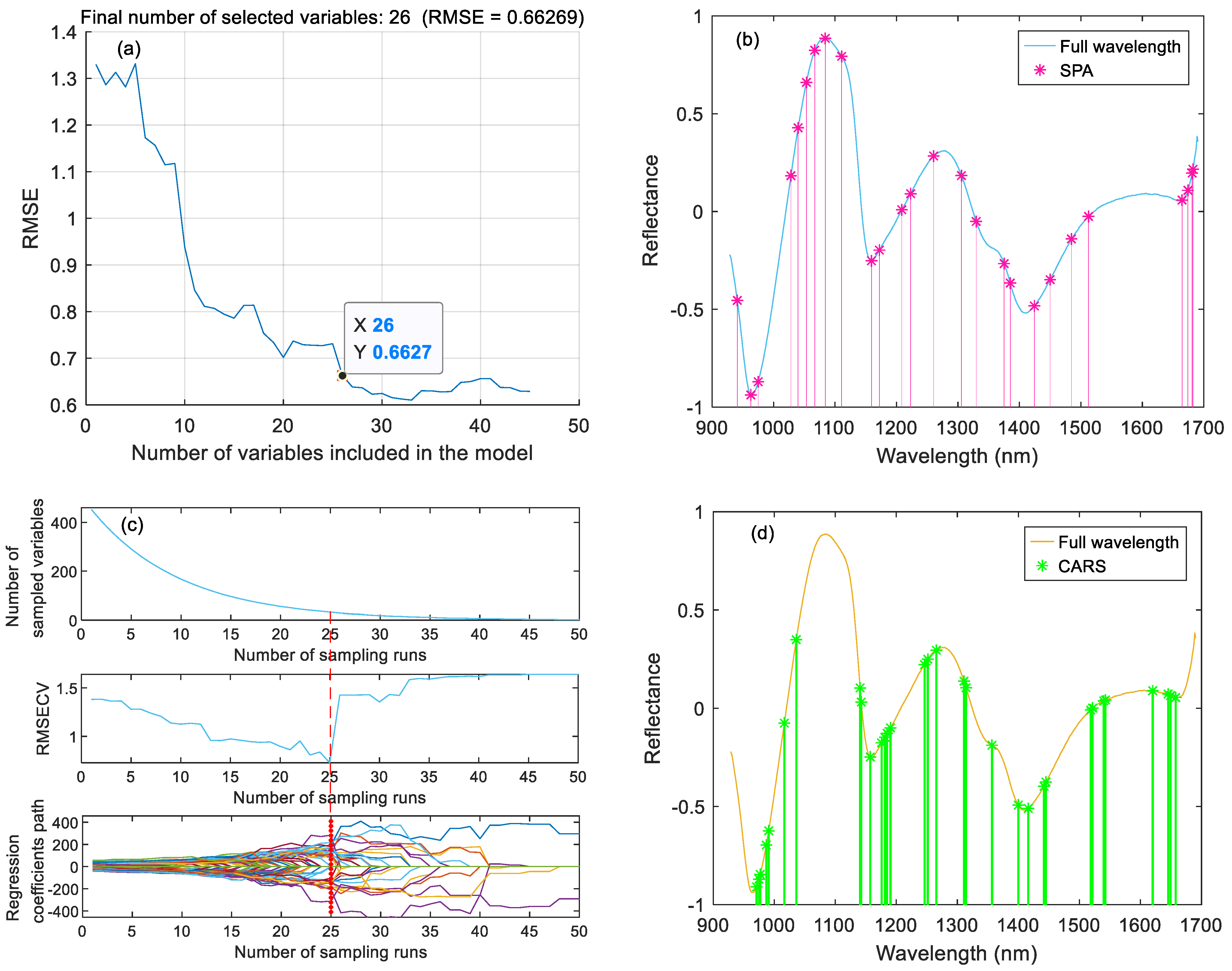
2.6.1. SPA
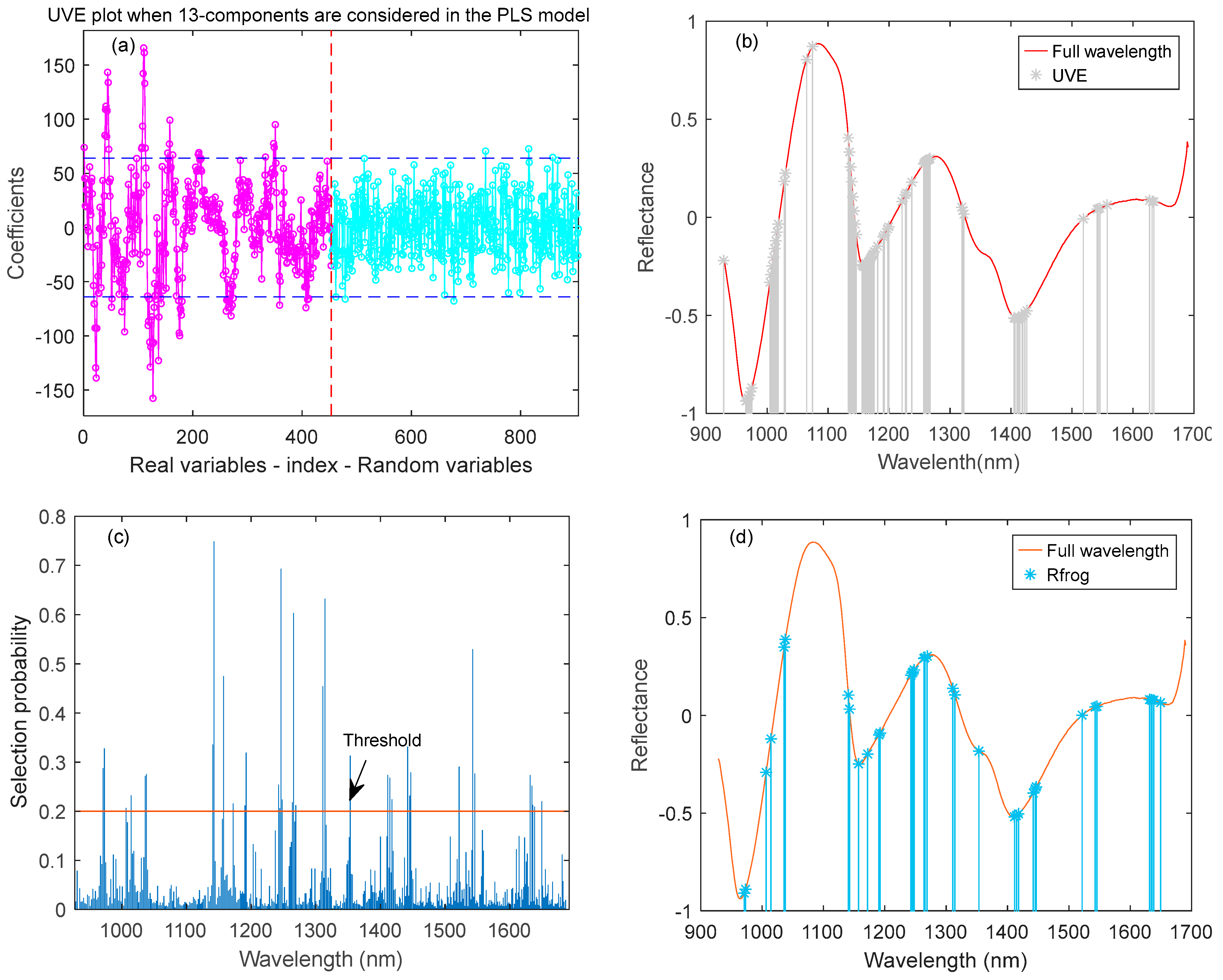
2.6.2. UVE
2.6.3. CARS
2.6.4. R-Frog
2.6.5. VCPA-IRIV
2.7. Modeling Algorithm
2.7.1. PLSR
2.7.2. BPNN
2.7.3. ELM
2.8. Evaluation Indicator
2.9. Model Explanation
3. Results and Discussion
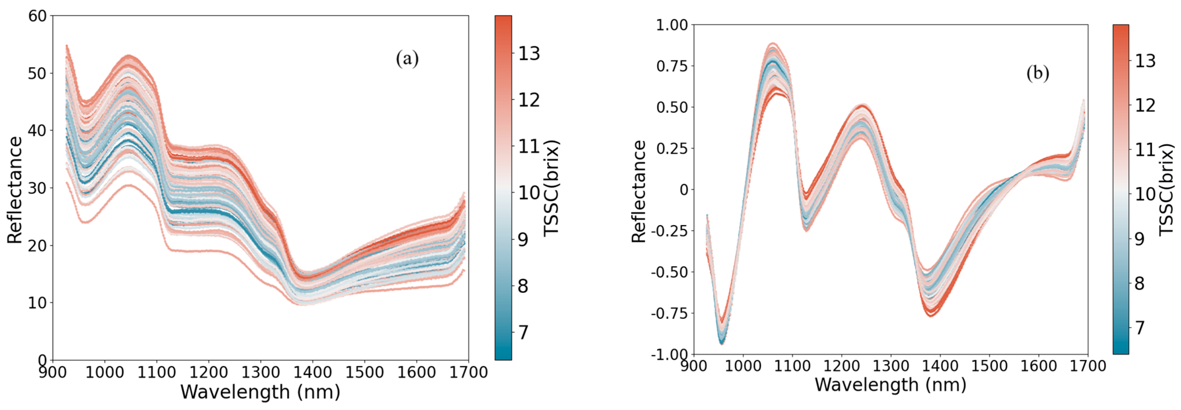
3.1. Spectral Interpretation
3.2. Preprocessing
3.3. Feature Variable Selection
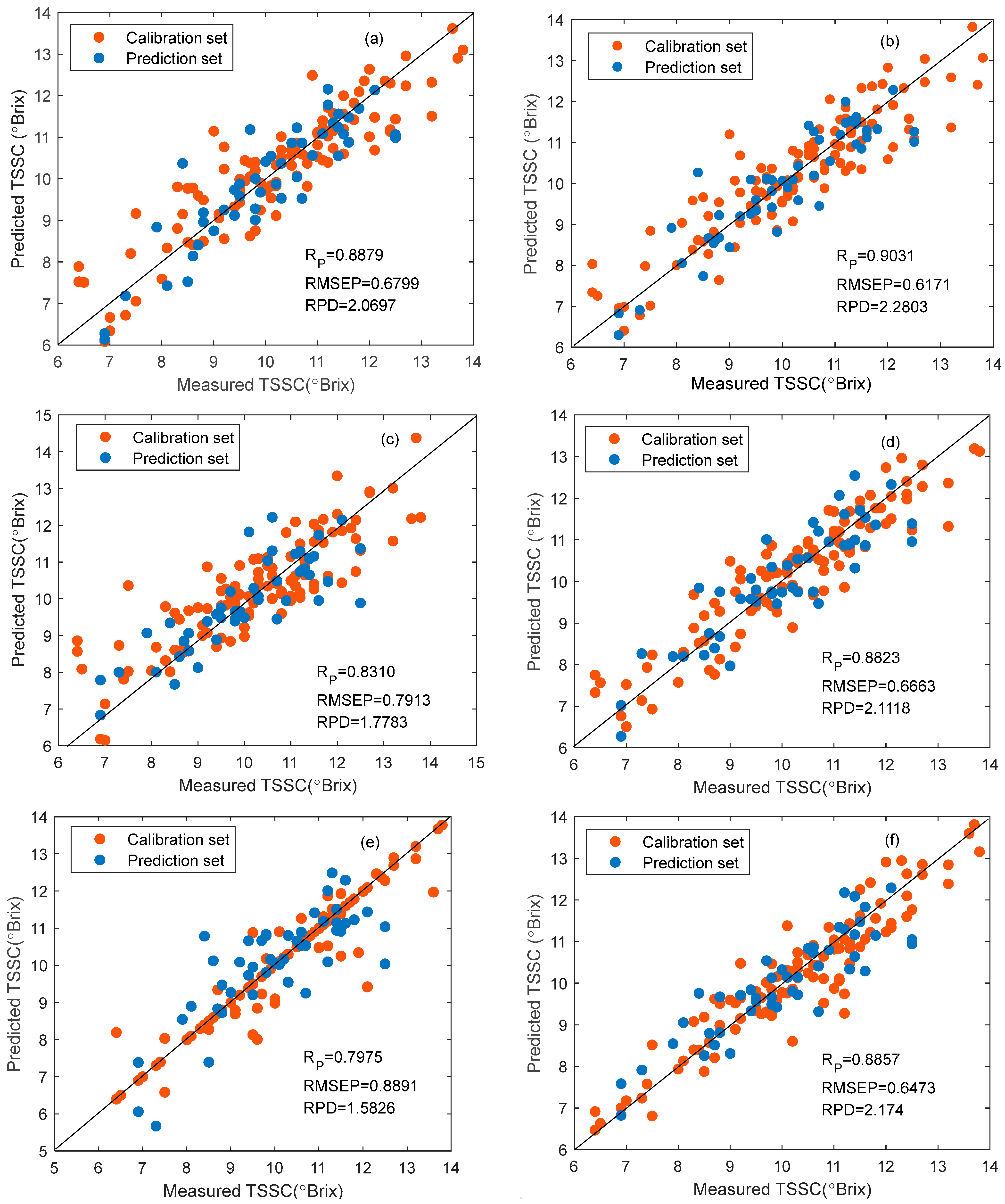
3.4. Modeling and Results
3.5. Explainable Analysis
4. Conclusions
Author Contributions
Funding
Institutional Review Board Statement
Informed Consent Statement
Data Availability Statement
Conflicts of Interest
References
- Gisbert, A.D.; Romero, C.; Martínez-Calvo, J.; Leida, C.; Llácer, G.; Badenes, M.L. Genetic Diversity Evaluation of a Loquat (Eriobotrya japonica (Thunb) Lindl) Germplasm Collection by SSRs and S-Allele Fragments. Euphytica 2009, 168, 121–134. [Google Scholar] [CrossRef]
- Zhu, N.; Nie, Y.; Wu, D.; He, Y.; Chen, K. Feasibility Study on Quantitative Pixel-Level Visualization of Internal Quality at Different Cross Sections Inside Postharvest Loquat Fruit. Food Anal. Methods 2017, 10, 287–297. [Google Scholar] [CrossRef]
- Ren, G.; Liu, Y.; Ning, J.; Zhang, Z. Assessing Black Tea Quality Based on Visible–near Infrared Spectra and Kernel-Based Methods. J. Food Compos. Anal. 2021, 98, 103810. [Google Scholar] [CrossRef]
- Ren, G.; Sun, Y.; Li, M.; Ning, J.; Zhang, Z. Cognitive Spectroscopy for Evaluating Chinese Black Tea Grades (Camellia sinensis): Near-infrared Spectroscopy and Evolutionary Algorithms. J. Sci. Food Agric. 2020, 100, 3950–3959. [Google Scholar] [CrossRef] [PubMed]
- Ren, G.; Wang, Y.; Ning, J.; Zhang, Z. Highly Identification of Keemun Black Tea Rank Based on Cognitive Spectroscopy: Near Infrared Spectroscopy Combined with Feature Variable Selection. Spectroc. Acta Part A Molec. Biomolec. Spectr. 2020, 230, 118079. [Google Scholar] [CrossRef]
- Nie, L.; Dai, Z.; Ma, S. Enhanced Accuracy of Near-Infrared Spectroscopy for Traditional Chinese Medicine with Competitive Adaptive Reweighted Sampling. Anal. Lett. 2016, 49, 2259–2267. [Google Scholar] [CrossRef]
- Zeng, S.; Zhang, Z.; Cheng, X.; Cai, X.; Cao, M.; Guo, W. Prediction of Soluble Solids Content Using Near-Infrared Spectra and Optical Properties of Intact Apple and Pulp Applying PLSR and CNN. Spectroc. Acta Part A Molec. Biomolec. Spectr. 2024, 304, 123402. [Google Scholar] [CrossRef] [PubMed]
- Praiphui, A.; Kielar, F. Comparing the Performance of Miniaturized Near-Infrared Spectrometers in the Evaluation of Mango Quality. Food Meas. 2023, 17, 5886–5902. [Google Scholar] [CrossRef]
- Qi, H.; Shen, C.; Chen, G.; Zhang, J.; Chen, F.; Li, H.; Zhang, C. Rapid and Non-Destructive Determination of Soluble Solid Content of Crown Pear by Visible/near-Infrared Spectroscopy with Deep Learning Regression. J. Food Compos. Anal. 2023, 123, 105585. [Google Scholar] [CrossRef]
- Lee, J.S.; Kim, S.-C.; Seong, K.C.; Kim, C.-H.; Um, Y.C.; Lee, S.-K. Quality Prediction of Kiwifruit Based on Near Infrared Spectroscopy. Hort. Sci. Technol. 2012, 30, 709–717. [Google Scholar] [CrossRef]
- Han, Z.; Li, B.; Wang, Q.; Yang, A.; Liu, Y. Detection Storage Time of Mild Bruise’s Loquats Using Hyperspectral Imaging. J. Spectrosc. 2022, 2022, 1–9. [Google Scholar] [CrossRef]
- Yin, H.; Li, B.; Liu, Y.; Zhang, F.; Su, C.; Ou-yang, A. Detection of Early Bruises on Loquat Using Hyperspectral Imaging Technology Coupled with Band Ratio and Improved Otsu Method. Spectroc. Acta Part A Molec. Biomolec. Spectr. 2022, 283, 121775. [Google Scholar] [CrossRef]
- Ore Areche, F.; Flores, D.D.C.; Quispe-Solano, M.A.; Nayik, G.A.; Cruz-Porta, E.A.D.L.; Rodríguez, A.R.; Roman, A.V.; Chweya, R. Formulation, Characterization, and Determination of the Rheological Profile of Loquat Compote Mespilus germánica L. through Sustenance Artificial Intelligence. J. Food Qual. 2023, 2023, 1–12. [Google Scholar] [CrossRef]
- Sun, J.; Yang, W.; Feng, M.; Liu, Q.; Kubar, M.S. An Efficient Variable Selection Method Based on Random Frog for the Multivariate Calibration of NIR Spectra. RSC Adv. 2020, 10, 16245–16253. [Google Scholar] [CrossRef] [PubMed]
- Yun, Y.; Bin, J.; Liu, D.; Xu, L.; Yan, T.; Cao, D.; Xu, Q. A Hybrid Variable Selection Strategy Based on Continuous Shrinkage of Variable Space in Multivariate Calibration. Anal. Chim. Acta 2019, 1058, 58–69. [Google Scholar] [CrossRef] [PubMed]
- Tan, F.; Mo, X.; Ruan, S.; Yan, T.; Xing, P.; Gao, P.; Xu, W.; Ye, W.; Li, Y.; Gao, X.; et al. Combining Vis-NIR and NIR Spectral Imaging Techniques with Data Fusion for Rapid and Nondestructive Multi-Quality Detection of Cherry Tomatoes. Foods 2023, 12, 3621. [Google Scholar] [CrossRef]
- De Oliveira, G.A.; Bureau, S.; Renard, C.M.-G.C.; Pereira-Netto, A.B.; De Castilhos, F. Comparison of NIRS Approach for Prediction of Internal Quality Traits in Three Fruit Species. Food Chem. 2014, 143, 223–230. [Google Scholar] [CrossRef] [PubMed]
- Zhao, M.; Cang, H.; Chen, H.; Zhang, C.; Yan, T.; Zhang, Y.; Gao, P.; Xu, W. Determination of Quality and Maturity of Processing Tomatoes Using Near-Infrared Hyperspectral Imaging with Interpretable Machine Learning Methods. LWT-Food Sci. Technol. 2023, 183, 114861. [Google Scholar] [CrossRef]
- Akulich, F.; Anahideh, H.; Sheyyab, M.; Ambre, D. Explainable Predictive Modeling for Limited Spectral Data. Chemom. Intell. Lab. Syst. 2022, 225, 104572. [Google Scholar] [CrossRef]
- Ahmed, M.T.; Villordon, A.; Kamruzzaman, M. Hyperspectral Imaging and Explainable Deep-Learning for Non-Destructive Quality Prediction of Sweetpotato. Postharvest Biol. Technol. 2025, 222, 113379. [Google Scholar] [CrossRef]
- Zhang, G.; Abdulla, W. Explainable AI-Driven Wavelength Selection for Hyperspectral Imaging of Honey Products. Food Chem. Adv. 2023, 3, 100491. [Google Scholar] [CrossRef]
- Zhong, L.; Guo, X.; Ding, M.; Ye, Y.; Jiang, Y.; Zhu, Q.; Li, J. SHAP Values Accurately Explain the Difference in Modeling Accuracy of Convolution Neural Network between Soil Full-Spectrum and Feature-Spectrum. Comput. Electron. Agric. 2024, 217, 108627. [Google Scholar] [CrossRef]
- Fang, S.; Wu, S.; Chen, Z.; He, C.; Lin, L.L.; Ye, J. Recent Progress and Applications of Raman Spectrum Denoising Algorithms in Chemical and Biological Analyses: A Review. TrAC Trends Anal. Chem. 2024, 172, 117578. [Google Scholar] [CrossRef]
- Yang, Z.; Nascimento, Y.M.; Monteiro, J.D.; Alves, B.E.B.; Melo, M.F.; Paiva, A.A.P.; Pereira, H.W.B.; Medeiros, L.G.; Morais, I.C.; Fagundes Neto, J.C.; et al. Fast Determination of Oxides Content in Cement Raw Meal Using NIR Spectroscopy with SPXY Algorithm. Anal. Methods 2018, 10, 1280–1285. [Google Scholar] [CrossRef]
- Galvao, R.; Araujo, M.; Jose, G.; Pontes, M.; Silva, E.; Saldanha, T. A Method for Calibration and Validation Subset Partitioning. Talanta 2005, 67, 736–740. [Google Scholar] [CrossRef]
- Li, H.; Liang, Y.; Xu, Q.; Cao, D. Key Wavelengths Screening Using Competitive Adaptive Reweighted Sampling Method for Multivariate Calibration. Anal. Chim. Acta 2009, 648, 77–84. [Google Scholar] [CrossRef]
- Sarkheyli, A.; Zain, A.M.; Sharif, S. The Role of Basic, Modified and Hybrid Shuffled Frog Leaping Algorithm on Optimization Problems: A Review. Soft Comput. 2015, 19, 2011–2038. [Google Scholar] [CrossRef]
- Guo, J.; Huang, H.; He, X.; Cai, J.; Zeng, Z.; Ma, C.; Lü, E.; Shen, Q.; Liu, Y. Improving the Detection Accuracy of the Nitrogen Content of Fresh Tea Leaves by Combining FT-NIR with Moisture Removal Method. Food Chem. 2023, 405, 134905. [Google Scholar] [CrossRef]
- Zhang, H.; Zhan, B.; Pan, F.; Luo, W. Determination of Soluble Solids Content in Oranges Using Visible and near Infrared Full Transmittance Hyperspectral Imaging with Comparative Analysis of Models. Postharvest Biol. Technol. 2020, 163, 111148. [Google Scholar] [CrossRef]
- Yin, H.; Ma, F.; Wang, D.; He, X.; Yin, Y.; Song, C.; Zhao, L. Establishing a Prediction Model for Tea Leaf Moisture Content Using the Free-Space Method’s Measured Scattering Coefficient. Agriculture 2023, 13, 1136. [Google Scholar] [CrossRef]
- Lundberg, S.M.; Lee, S.-I. A Unified Approach to Interpreting Model Predictions. Neural Inf. Process. Syst. 2017, 30, 4765–4774. [Google Scholar]
- Yu, K.; Zhao, Y.; Liu, Z.; Li, X.; Liu, F.; He, Y. Application of Visible and Near-Infrared Hyperspectral Imaging for Detection of Defective Features in Loquat. Food Bioprocess Technol. 2014, 7, 3077–3087. [Google Scholar] [CrossRef]
- Yuan, L.; You, L.; Yang, X.; Chen, X.; Huang, G.; Chen, X.; Shi, W.; Sun, Y. Consensual Regression of Soluble Solids Content in Peach by Near Infrared Spectrocopy. Foods 2022, 11, 1095. [Google Scholar] [CrossRef] [PubMed]
- Luo, W.; Zhang, J.; Liu, S.; Huang, H.; Zhan, B.; Fan, G.; Zhang, H. Prediction of Soluble Solid Content in Nanfeng Mandarin by Combining Hyperspectral Imaging and Effective Wavelength Selection. J. Food Compos. Anal. 2024, 126, 105939. [Google Scholar] [CrossRef]
- Çifci, A.; Kırbaş, İ. Fusion of Machine Learning and Explainable AI for Enhanced Rice Classification: A Case Study on Cammeo and Osmancik Species. Eur. Food Res. Technol. 2024. [Google Scholar] [CrossRef]
- Zhao, Y.; Zhang, C.; Zhu, S.; Li, Y.; He, Y.; Liu, F. Shape Induced Reflectance Correction for Non-Destructive Determination and Visualization of Soluble Solids Content in Winter Jujubes Using Hyperspectral Imaging in Two Different Spectral Ranges. Postharvest Biol. Technol. 2020, 161, 111080. [Google Scholar] [CrossRef]
- Sharma, A.; Kumar, R.; Kumar, N.; Kaur, K.; Saxena, V.; Ghosh, P. Chemometrics Driven Portable Vis-SWNIR Spectrophotometer for Non-Destructive Quality Evaluation of Raw Tomatoes. Chemom. Intell. Lab. Syst. 2023, 242, 105001. [Google Scholar] [CrossRef]


| Data Set | Number of Samples | Min (%) | Max (%) | Mean (%) | Std/(%) |
|---|---|---|---|---|---|
| Prediction set | 47 | 6.9 | 12.5 | 10.02 | 1.39 |
| Calibration Set | 109 | 6.4 | 13.8 | 10.23 | 1.65 |
| Number | Preprocessing Method | LVs | RMSEC | RMSEP | RPD | ||
|---|---|---|---|---|---|---|---|
| 1 | Raw | 14 | 0.9762 | 0.3576 | 0.8258 | 0.8226 | 1.7105 |
| 2 | SG(3) | 11 | 0.9077 | 0.6916 | 0.8614 | 0.7184 | 1.9587 |
| 3 | SG(7) | 11 | 0.9030 | 0.7082 | 0.8623 | 0.7189 | 1.9574 |
| 4 | SG(7)-DT | 11 | 0.9095 | 0.6849 | 0.8764 | 0.7123 | 1.9753 |
| 5 | SG(7)-SNV | 11 | 0.9148 | 0.6657 | 0.8626 | 0.7340 | 1.9171 |
| 6 | SG(7)-MSC | 11 | 0.9100 | 0.6832 | 0.8722 | 0.7103 | 1.9809 |
| 7 | SG(7)-SNV-DT | 10 | 0.9020 | 0.7117 | 0.8879 | 0.6799 | 2.0697 |
| 8 | SG(7)-MSC-DT | 10 | 0.9033 | 0.7069 | 0.8870 | 0.8043 | 1.7495 |
| Model | Wavelength Selection | Calibration Set | Validation Set | |||
|---|---|---|---|---|---|---|
| RMSEC | RMSEP | RPD | ||||
| PLSR | Full-spectrum | 0.9020 | 0.7117 | 0.8879 | 0.6799 | 2.0697 |
| SPA | 0.9059 | 0.6980 | 0.9031 | 0.6171 | 2.2803 | |
| UVE | 0.9106 | 0.6811 | 0.8733 | 0.7206 | 1.9527 | |
| CARS | 0.9564 | 0.4812 | 0.8583 | 0.7964 | 1.7668 | |
| R-Frog | 0.9314 | 0.5997 | 0.8505 | 0.8016 | 1.7553 | |
| UVE-SPA | 0.8915 | 0.7466 | 0.8752 | 0.6951 | 2.0244 | |
| VCPA-IRIV | 0.9189 | 0.6500 | 0.8783 | 0.6919 | 2.0126 | |
| ELM | Full-spectrum | 0.8577 | 0.8475 | 0.8310 | 0.7913 | 1.7783 |
| SPA | 0.8453 | 0.8804 | 0. 8601 | 0.7398 | 1.9019 | |
| UVE | 0.9283 | 0.6126 | 0.8823 | 0.6663 | 2.1118 | |
| CARS | 0.9453 | 0.5375 | 0.8647 | 0.7261 | 1.9378 | |
| R-Frog | 0.9190 | 0.6497 | 0.8359 | 0.8409 | 1.6734 | |
| UVE-SPA | 0.8825 | 0.7750 | 0.8499 | 0.7425 | 1.8952 | |
| VCPA-IRV | 0.9214 | 0.6403 | 0.8741 | 0.6854 | 2.0529 | |
| BPNN | Full-spectrum | 0.9488 | 0.5312 | 0.7975 | 0.8891 | 1.5826 |
| SPA | 0.9057 | 0.7006 | 0.8584 | 0.7449 | 1.8889 | |
| UVE | 0.8573 | 0.8663 | 0.8543 | 0.7996 | 1.7597 | |
| CARS | 0.9613 | 0.4594 | 0.8663 | 0.7194 | 1.9559 | |
| R-Frog | 0.9388 | 0.6091 | 0.8250 | 0.8156 | 1.7252 | |
| UVE-SPA | 0.9189 | 0.7161 | 0.8335 | 0.9223 | 1.5257 | |
| VCPA-IRIV | 0.9411 | 0.5639 | 0.8857 | 0.6473 | 2.1740 | |
Disclaimer/Publisher’s Note: The statements, opinions and data contained in all publications are solely those of the individual author(s) and contributor(s) and not of MDPI and/or the editor(s). MDPI and/or the editor(s) disclaim responsibility for any injury to people or property resulting from any ideas, methods, instructions or products referred to in the content. |
© 2025 by the authors. Licensee MDPI, Basel, Switzerland. This article is an open access article distributed under the terms and conditions of the Creative Commons Attribution (CC BY) license (https://creativecommons.org/licenses/by/4.0/).
Share and Cite
Luo, Y.; Jin, Q.; Lu, H.; Li, P.; Qiu, G.; Qi, H.; Li, B.; Zhou, X. Advancing Loquat Total Soluble Solids Content Determination by Near-Infrared Spectroscopy and Explainable AI. Agriculture 2025, 15, 281. https://doi.org/10.3390/agriculture15030281
Luo Y, Jin Q, Lu H, Li P, Qiu G, Qi H, Li B, Zhou X. Advancing Loquat Total Soluble Solids Content Determination by Near-Infrared Spectroscopy and Explainable AI. Agriculture. 2025; 15(3):281. https://doi.org/10.3390/agriculture15030281
Chicago/Turabian StyleLuo, Yizhi, Qingting Jin, Huazhong Lu, Peng Li, Guangjun Qiu, Haijun Qi, Bin Li, and Xingxing Zhou. 2025. "Advancing Loquat Total Soluble Solids Content Determination by Near-Infrared Spectroscopy and Explainable AI" Agriculture 15, no. 3: 281. https://doi.org/10.3390/agriculture15030281
APA StyleLuo, Y., Jin, Q., Lu, H., Li, P., Qiu, G., Qi, H., Li, B., & Zhou, X. (2025). Advancing Loquat Total Soluble Solids Content Determination by Near-Infrared Spectroscopy and Explainable AI. Agriculture, 15(3), 281. https://doi.org/10.3390/agriculture15030281