A Skeleton-Based Method of Root System 3D Reconstruction and Phenotypic Parameter Measurement from Multi-View Image Sequence

Abstract

The phenotypic parameters of root systems are vital in reflecting the influence of genes and the environment on plants, and three-dimensional (3D) reconstruction is an important method for obtaining phenotypic parameters. Based on the characteristics of root systems, being featureless, thin structures, this study proposed a skeleton-based 3D reconstruction and phenotypic parameter measurement method for root systems using multi-view images. An image acquisition system was designed to collect multi-view images for root system. The input images were binarized by the proposed OTSU-based adaptive threshold segmentation method. Vid2Curve was adopted to realize the 3D reconstruction of root systems and calibration objects, which was divided into four steps: skeleton curve extraction, initialization, skeleton curve estimation, and surface reconstruction. Then, to extract phenotypic parameters, a scale alignment method based on the skeleton was realized using DBSCAN and RANSAC. Furthermore, a small-sized root system point completion algorithm was proposed to achieve more complete root system 3D models. Based on the above-mentioned methods, a total of 30 root samples of three species were tested. The results showed that the proposed method achieved a skeleton projection error of 0.570 pixels and a surface projection error of 0.468 pixels. Root number measurement achieved a precision of 0.97 and a recall of 0.96, and root length measurement achieved an MAE of 1.06 cm, an MAPE of 2.37%, an RMSE of 1.35 cm, and an R² of 0.99. The whole process of reconstruction in the experiment was very fast, taking a maximum of 4.07 min. With high accuracy and high speed, the proposed methods make it possible to obtain the root phenotypic parameters quickly and accurately and promote the study of root phenotyping.

1. Introduction

Plant’s root systems are an important multifunctional nutrient organ that participates in various life functions of plants and provides stability and support. Recent research has found that root phenotypic parameters can reflect the growth status of plants. Meanwhile, there is a certain correlation between root phenotypic parameters and yield [1,2,3]. Therefore, obtaining root phenotypic parameters can help people discover the close relationship between root growth and the environment, address specific issues in agricultural production, and promote the development of modern agricultural science.

Traditional methods for obtaining root phenotypic parameters mainly rely on manual measurement, which is time-consuming and has low accuracy. With the development of image processing technology, 2D images have widely been used in root phenotyping. Researchers have used methods such as germination paper [4], rhizoponics setup [5], and agar plates [6] to visualize the growth processes of root systems and obtain 2D root system images with RGB cameras and scanners. Then, threshold segmentation [7,8,9] or deep learning networds, such as UNet [10,11], SE-ResNet [12] and the GAN [13] network, were used to process the images. These methods, using the 2D images, showed great advantages, with their characteristic low costs, but they still had certain limitations. Firstly, the 2D images could only capture a projected view of the root system, which failed to represent the complex, three-dimensional nature of roots. This resulted in the loss of important spatial information. Secondly, due to occlusion and ambiguity issues caused by perspective projection, the methods based on 2D images often suffered from measurement inaccuracies. Thirdly, many phenotypic parameters of roots are difficult to quantify based only on 2D images.

With the development of artificial intelligence, many new 3D reconstruction methods have emerged and been applied more and more widely in the field of agriculture [14,15]. For root phenotyping, 3D reconstruction methods can provide a more comprehensive, accurate, and detailed representation of the root system’s spatial configuration. Three-dimensional reconstruction technology is mainly divided into active and passive methods. Active methods include CT [16,17,18], MRI [19,20] and laser imaging [21,22,23], and are widely used to reconstruct root system 3D models, obtain root phenotypic parameters [24,25], and realize early disease detection [26]. The accuracies of active methods are high, but they are time- and cost-consuming, with low practical value. Passive methods realizing 3D reconstruction mainly depend on feature signals of 2D images. A typical passive method for root system 3D reconstruction is Structure-from-Motion (SFM), based on feature points which uses visual feature points in images and then identify the dense point correspondences between texture features. SFM, based on feature points for 3D root system reconstruction, were mostly used when the root system was relatively thick, such as the root systems of rape and maize in the late growth period [27] and cassava root crown [28]. While the root systems of many plants tend to be fine and complex with various branches, and lack texture features [29], as featureless, thin structures, feature point matching may be caused to fail [30], and the reconstruction effect in SFM based on feature points may be reduced.

To reconstruct thin structures which are featureless, thin objects, and only a few pixels wide in the images, there have been some curve-based reconstruction works. But some have struggled with inaccurate camera pose predictions [31,32,33], and some required pre-computed camera poses as input [34,35]. Vid2Curve [36] was an iterative optimization method based on skeleton curves to reconstruct 3D thin structures. Without requiring visual texture features or point features in the background scene and pre-calibrated camera poses, it established correspondences between skeleton curves of featureless, thin objects in the foreground in consecutive multi-view images, which can help in achieving high quality reconstructions of complex 3D wire models.

Based on the characteristics of root systems, being thin structures which lacking surface textural features, this study proposed a skeleton-based 3D reconstruction and phenotypic measurement method for root systems which includes (1) designing an image acquisition system to collect multi-view images for 3D root system reconstructions, (2) proposing an OTSU-based adaptive threshold segmentation method, (3) adopting a Vid2Curve method for root system 3D reconstruction from multi-view image sequences, (4) realizing scale alignment by way of a self-designed calibration object based on clustering and linear fitting of skeleton points, (5) proposing a small-sized root system point completion algorithm. Experiments were conducted using the proposed method to evaluate the reconstruction quality and accuracy of phenotypic parameters compared to the ground truth value.

2. Materials and Methods

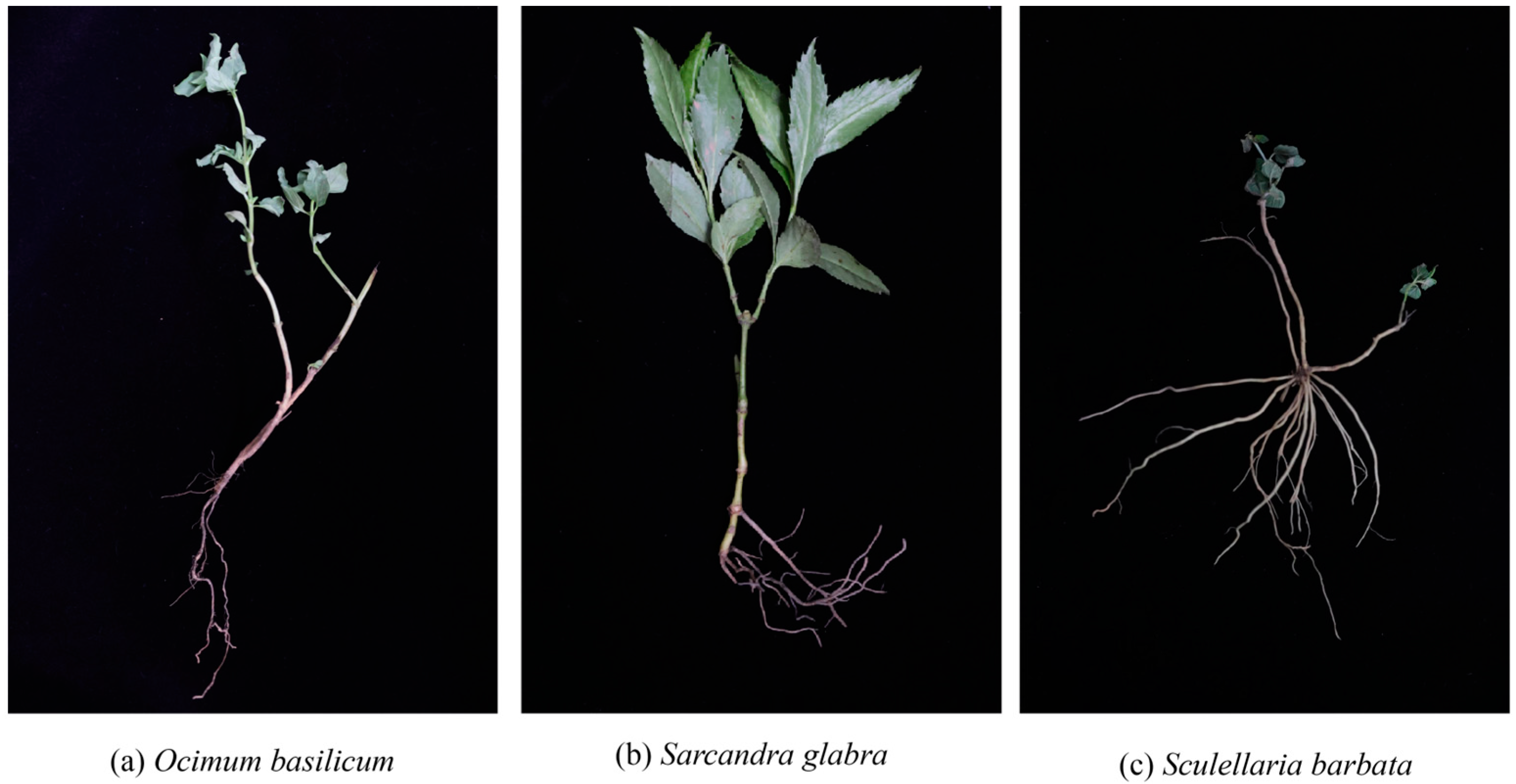
2.1. Samples

To demonstrate the robustness of the 3D reconstruction method, three species of herb root systems in the seedling stage, as shown in Figure 1, including Ocimum basilicum roots which were marked as Ob, Sarcandra glabra roots which were marked as Sg, and Sculellaria barbata roots which were marked as Sb, were chosen in this study. The root system of each species exhibited unique characteristics. Ocimum basilicum is straight root plant, whose root system in the seedling stage consists of a conical taproot and fibrous roots, with the taproot possessing high structural strength. Sarcandra glabra is whisker root plant, whose root system in the seedling stage is fibrous and relatively dense, with high structural strength, making it less prone to mutual shading. Sculellaria barbata is whisker root plant, whose root system in the seedling stage is mainly composed of clustered, slender, and fibrous roots, exhibiting low structural strength and severe shading between roots. In this study, the ground truth values for root phenotypic parameters were obtained by manual measurement. After collecting the root system images, the root numbers were manually counted. Subsequently, the root systems of each sample were destructively sampled, each root was straightened, and each root was then measured with a vernier caliper. The sum of each root length was taken as the total root length for each sample.

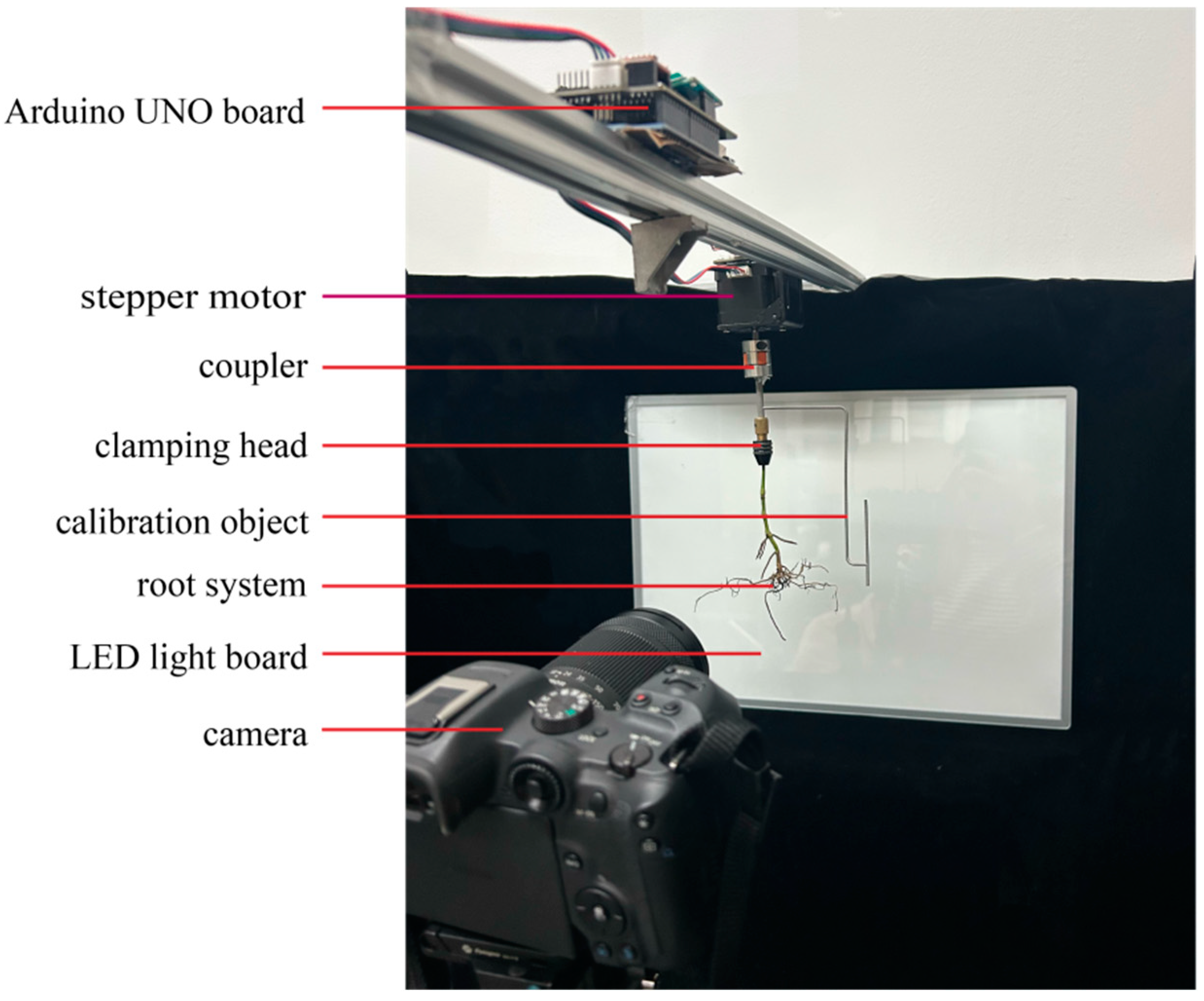
2.2. Experiment System

The proposed multi-view image acquisition system for 3D root system reconstruction was designed and constructed as shown in Figure 2. The image acquisition system included a stepper motor, Arduino UNO board, coupler, calibration object, clamping head, LED light board, camera (Canon R7), and aluminum alloy sections. The stepper motor was controlled by the Arduino UNO board, the coupler was used to connect the motor to the calibration object, and the clamping head was used to clamp the root system. For scale alignment, a calibration object which was also a thin structure was designed. To facilitate the segmentation of the root system and the calibration object, marked as target object, from the background, an LED light board was used to provide backlight. The motor and Arduino UNO board were fixed onto a frame constructed with aluminum alloy sections. The stepper motor, coupler, calibration object, and clamping head were connected in sequence. During data acquisition, the stepper motor drove the rotation of the target object, and the camera was fixed on one side, capturing multi-view images of the target object.

2.3. Image Preprocessing

After acquiring multi-view images of the target object with a resolution of 1920 × 1080 using the image acquisition system, the images were downsampled to a resolution of 960 × 540 to ensure the speed and accuracy of reconstruction. The images were then segmented to obtain binary masks of the pixels showing the target object in the foreground. To ensure the accuracy of the segmentation, a backlight was used to increase the contrast between the background and the target object. The OTSU algorithm is a threshold selection method from gray-level histograms [37]. It is suitable for high-contrast images. However, many root samples exhibited significant variation in root diameter, and slight vibrations might occur during the rotation of the root system, both of which could easily lead to inaccurate OTSU segmentation.

To address this, an OTSU-based adaptive threshold segmentation algorithm was designed, as seen in Figure 3. First, the grayscale matrix of the original image was obtained. Then, the grayscale matrix was binarized as $G$ by OTSU algorithm: for each pixel, if its gray value in the grayscale matrix was below the global threshold, it was classified as the target area, setting its gray value to 0, or setting its gray value to 255. At the same time, the box filter method was used to perform mean smoothing on the grayscale matrix, and the grayscale matrix was subtracted from the smoothed result to obtain a filtered matrix. The filtered matrix was binarized as $F$ by the following process: for each pixel, if its gray value in the filtered matrix was below the 0, its gray value would be set to 0, or its gray value would be set to 255. Finally, the final matrix $R$ was calculated by Equation (1) as the result. Through this process, an accurate binary mask of the pixels showing the target object in the foreground could be obtained.

$$R=G\odot F$$

(1)

2.4. Skeleton-Based 3D Reconstruction

The vast majority of roots had circular cross-sections, and the root systems could be seen as collections of connected, generalized cylinders. Vid2Curve was an iterative optimization method based on 2D skeleton curves and the distances from the 2D skeleton point to both sides of the strip in each view to estimate accurate camera poses and reconstruct thin 3D structures without the use of color and texture information, and, additionally, there was no need to pre-calibrate the input images. This made it possible to reconstruct the seedling root system in minutes.

The Vid2Curve algorithm was mainly divided into four steps, as shown in Figure 4: skeleton curve extraction, initialization, skeleton curve estimation by iteration, and surface reconstruction.

(1)

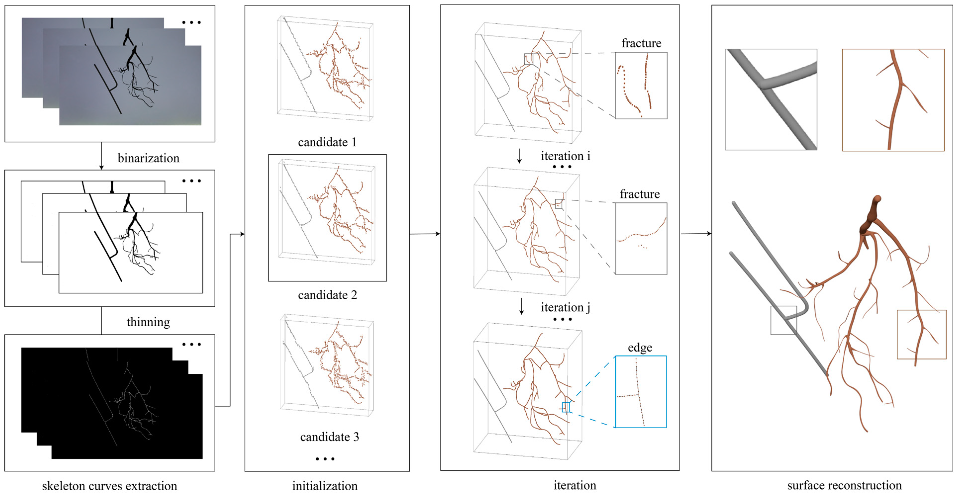
The binary masks of the pixels showing the target object in the foreground were processed by thinning method to extract on pixel wide skeleton curves which were henceforth denoted by $c=\{c_k\in R^2,k=1,2,\dots ,K\}$. And the input views were denoted by $I=\{I_k,k=1,2,\dots ,K\}$.

(2)

By using the optical flow method and bundle adjustment from the first few pictures, several 3D points candidates were initialized, and the best-performing 3D points candidates, henceforth denoted by $P=\{P_i\in R^3,i=1,2,\dots ,x\}$, were selected as a basis for subsequent iterations.

(3)

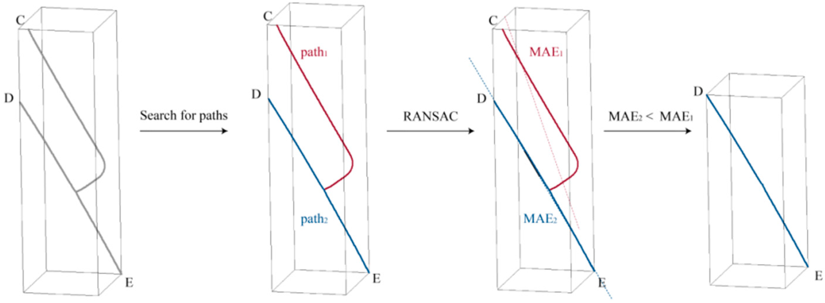
The camera poses $(R_k,T_k)$ and the curve network $C$ were computed by minimizing an objective function (Equation (2)) that measured the sum of the squared 2D distances between the projection of the curve network, $C$, and the corresponding 2D skeletal curve, $c_k$, across all input pictures. And, a commonly used formulation for curve fitting was utilized to efficiently minimize the distance error term $e_{k,j}$ (Equation (3)). The function was minimized iteratively in an alternating fashion that first optimized the camera poses while fixing the curve points, and then optimized the curve points while fixing the camera poses. During the iteration, $P$ had to be matched with the points $Q=\{q_i\in R^2,i=1,2,\dots ,n\}$, in the view of $I_k$, and the matching was performed by combining a distance-based criterion with a constraint on curve consistency. During the initialization and iteration, $C$, which recorded the edges by pairing points, was constructed and updated based on 3D points through the variant of Kruskal’s algorithm, which determined whether the points were connected based on the distance between them and the length of the loop formed by the edges. At the same time, the 3D points were uniformly resampled. Also at the same time, there may be self-occlusion due to the root structure. To determine whether the 3D points were subject to self-occlusion in certain view $I_k$, the neighboring pixels of the matching point $q_i$ for each point $P_i$ would be examined with a 3 $\times$ 3 local window, and a 3D point set $\widehat{P}$ that matches the pixels would be generated. Then, the spatial compactness factor, ${\sigma }_i$, was computed from the average distance between the points in P and their centroid. If ${\sigma }_i<10/f_0$, $P_i$ was labeled as self-occluded, setting $\alpha$ to 0, or setting $\alpha$ to 1.

$$\tilde{F}(\{R_k,T_k\};C)={\displaystyle \sum _k{\displaystyle \sum _{P_j\in C}\alpha \cdot e_{k,j}+F_s(C)}}$$

(2)

$$e_{k,j}={‖(\pi (R_k{P}_j+T_k)-q_j)\cdot n_j‖}^2+0.5{‖(\pi (R_k{P}_j+T_k)-q_j)\cdot t_j‖}^2$$

(3)

$$F_s(C)={(2.5f_0)}^2{\displaystyle \sum _k{\displaystyle \sum _{P_j\in C}{‖P_{j+1}-2P_j+P_{j-1}‖}^2}}$$

(4)

where $\alpha$ was 0 if the point $P_j$ was self-occluded, and, otherwise, was 0. $e_{k,j}$ was distance error, and $n_j$ was the normal direction of the point $P_j$. $t_j$ was the tangent direction of the point $P_j$. $F_s(C)$ was regularization term, and $f_0$ was the focal length of the camera.

(4)

To reconstruct the root surface, the root system was considered to be composed of generalized cylinders, so the radius of each point was the key which was calculated using the corresponding image observations from all multi-view binary images. Specifically, the radius of $P_j$ was the average of the radii $r_j^k$ over all the input images.

$$r_j^k={\displaystyle \frac{{\overline{r}}_j^k}{f_0}}\cdot \mathrm{depth}(P_j,I_k)$$

(5)

where ${\overline{r}}_j^k$ was the distances from the projection point of $P_j$, in each view $I_k$, to both sides of the defined strip. $\mathrm{depth}(P_j,I_k)$ was the depth of $P_j$ with respect to the view $I_k$.

After completing the above steps, the skeleton reconstruction results and the surface reconstruction results for the root system were obtained.

2.5. Scale Alignment for Phenotypic Parameters Measurement

To extract root phenotypic parameters, achieving scale alignment was crucial. Many studies used a calibration board for camera calibration and pose determination [38], but using calibration board would complicate image segmentation. To achieve rapid scale alignment, this study achieved scale alignment by calculating the distance between two specific points on the calibration object, which can be reconstructed with the proposed reconstruction method. Figure 5a illustrated the calibration object, which was also a collection of connected generalized cylinders. Point A was the connection point between the calibration object and the motor, and point B was the connection point between the calibration object and the clamp. Point C represented the endpoint of the calibration object in the reconstruction result, the position of which was uncertain due to the rotation of the acquisition device and changes in the shooting angle during image acquisition. The distance between point D and point E on the calibration object was 8.5 cm, and the scale was obtained by calculating the ratio of the DE distance in the reconstruction result to the ground truth value.

In order to calculate the DE distance, the calibration object points needed to be segmented from the skeleton reconstruction results. To achieve segmentation, this study employed the DBSCAN [39] method for clustering points, as seen in Figure 6, considering that the points were resampled based on distance during reconstruction. The clustering result was classified according to the number of points, and the group with fewer points was the calibration object point cloud. Then, as in Figure 7, the calibration object point cloud was classified into two paths based on the connectivity of points, and linear fitting, based on RANSAC [40], was performed on two paths with calculated Mean Absolute Error (MAE) values. The path with the smaller MAE was identified as the DE segment point cloud. The length of the line connecting the DE segment point cloud was computed, and the scaling factor $\beta$ was derived using Equation (6).

$$\beta ={\displaystyle \frac{\widetilde{DE}}{DE}}$$

(6)

where $\widetilde{DE}$ was the DE distance in reconstruction result, $DE$ was the ground truth value.

2.6. Skeleton-Based Point Completion

In the 3D reconstruction of root systems, issues such as mutual occlusion between roots and vibration during rotation could lead to missing regions in the reconstruction results, which affect the calculation of phenotypic parameters. To obtain a more complete 3D model of the root system, point completion was performed based on the connectivity of the skeleton in the reconstruction results and the structural characteristics of the root system. This process mainly consisted of three steps: classifying the skeleton point cloud based on connectivity, finding connection points, and regenerating surfaces. The specific completion steps are as follows:

(1)

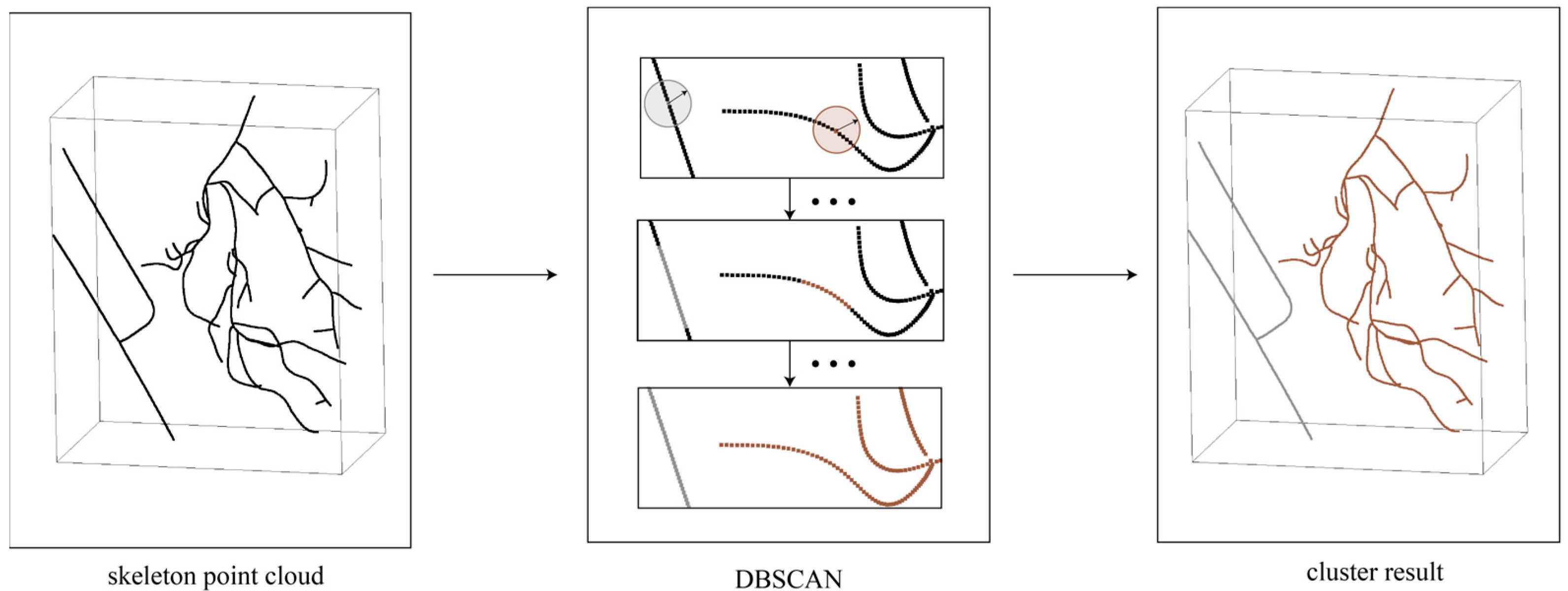
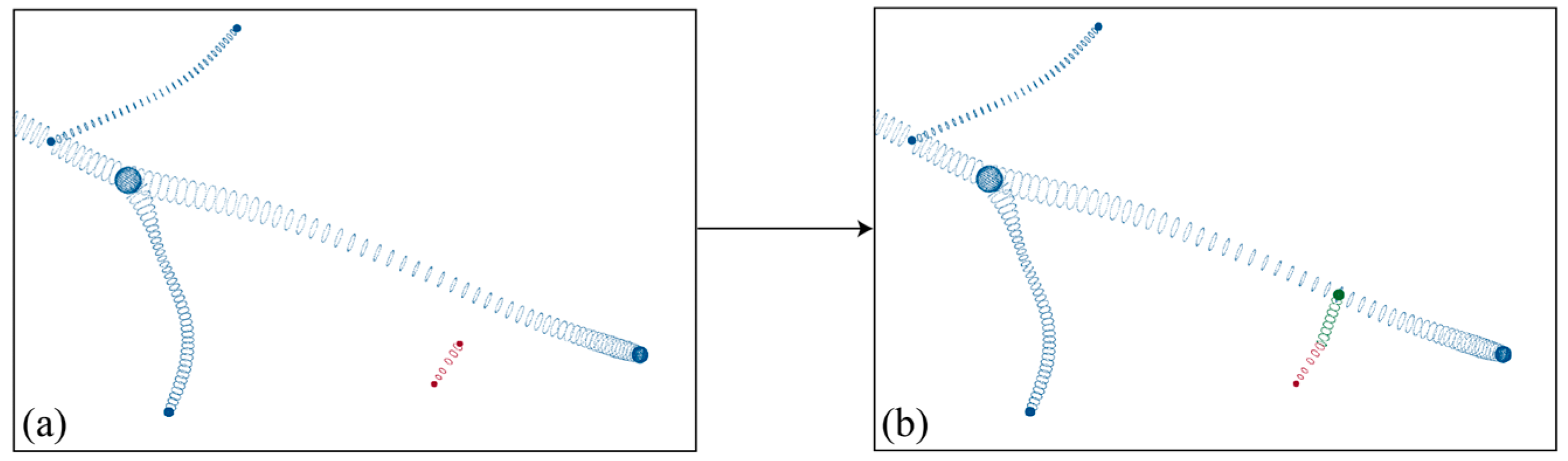
The connectivity of the reconstructed skeleton point cloud was determined based on the DFS algorithm, dividing the skeleton point cloud with a missing region into independent skeleton point clouds, as in Figure 8a,b. Based on the number of points, independent skeletons were classified into a primary skeleton and sub-skeletons, while also saving all endpoint coordinates, henceforth denoted by $M=\{m_i\in R^3,i=1,2,\dots ,n\}$.

(2)

For each sub-skeleton, through all endpoints $m_i$ are iterated through, and the tangent vector $\overrightarrow{m_i{t}_i}$ is found for $m_i$. As in Figure 8b, for each $m_i$, all points in the primary skeleton are traversed to find a point $r_i$ that satisfied Equation (7). If such a point is found, it is considered a candidate connection point, and the length of $m_i{r}_i$ is recorded. After completing the traversal, the shortest $m_i{r}_i$ is retained as the connection line, and $r_i$ is checked with regard to it being in the endpoint set. If so, it is removed. To ensure an even distribution of the skeleton point cloud, points were uniformly sampled along the $m_i{r}_i$ connection line at intervals of the average point distance, as in Figure 8c. At the same time, to ensure the smoothness of the skeleton, if $r_i$ is an endpoint, the points sampled along $m_i{r}_i$, and points of this sub-skeleton, are used for curve fitting. Then, points are uniformly sampled along the curve again, and the sampled points are added to the skeleton points. After traversing all sub-skeletons, the skeleton point completion was completed as Figure 8d.

(3)

To generate the surface, the radii of the points sampled on the $m_i{r}_i$ connection line were also required. To ensure the smoothness of the generated surface, if $r_i$ is an endpoint, the radius along the $m_i{r}_i$ connection line is then set to vary linearly with the radius of $m_i$ and $r_i$; if $r_i$ is not an endpoint, the radius along the $m_i{r}_i$ connection line is considered to be the same as at point $m_i$. Based on the completed skeleton points and the radius, surface generation can be accomplished, as seen in Figure 9.

$$\overrightarrow{m_i{r}_i}\cdot \overrightarrow{m_i{t}_i}\ge 0$$

(7)

2.7. Evaluation of Reconstruction Quality

Reconstruction accuracy was quantified by projection error (PE), including the skeleton projection error (SPE) and surface projection error (FPE). PE, demonstrating the consistency of projected points between the reconstruction results and the ground truth, was calculated by Equation (8). SPE, which can reflect the effect of reconstruction of the skeleton points, was used to calculate the average of the distances between the projection of points on the skeleton and the closet points sampled on 2D extracted skeletons over all multi-views. FPE, which can reflect the effect of reconstruction of the surface points, measured the average of distances between the projection of points on the reconstruction surface and the closet points sampled on input images over all multi-views. The average (AVG) was calculated to represent the average effect of reconstruction, and the standard deviation (SD) was calculated to represent the dispersion degree of reconstruction effect.

$$PE={\displaystyle \frac{{\displaystyle \sum _{i=1}^n\sqrt{{({\widehat{x}}_i-x_i)}^2+{({\widehat{y}}_i-y_i)}^2}}}{n}}$$

(8)

where $({\widehat{x}}_i,{\widehat{y}}_i)$ was the projected point of the reconstruction results and $(x_i,y_i)$ was the projected point of the ground truth.

In this study, root number and root length, chosen as the phenotypic parameters, were measured. Root number was given a value by counting the number of endpoints in the reconstruction result. And the precision and the recall were calculated to evaluate the bias of the root number.

$$precision={\displaystyle \frac{TP}{TP+FP}}$$

(9)

$$recall={\displaystyle \frac{TP}{TP+FN}}$$

(10)

where $TP$ was the number of correctly reconstructed roots in the reconstruction result and $FP$ was the number of incorrectly reconstructed roots in the reconstruction result. $FN$ was the number of roots that were not reconstructed in the reconstruction result.

Root length was measured by the length of skeleton lines combining with the scale factor $\beta$. The accuracy of the root length measurement was evaluated by MAE (Equation (11)), mean absolute percentage error (MAPE, Equation (12)), the root mean square error (RMSE, Equation (13)), and the R-squared (R², Equation (14)).

$$MAE={\displaystyle \sum _{i=1}^n\frac{\left|{\widehat{l}}_i-l_i\right|}{n}}\times 100\%$$

(11)

$$MAPE={\displaystyle \sum _{i=1}^n\left|\frac{{\widehat{l}}_i-l_i}{n{l}_i}\right|}\times 100\%$$

(12)

$$RMSE=\sqrt{{\displaystyle \sum _{i=1}^n\frac{{\left({\widehat{l}}_i-l_i\right)}^2}{n}}}$$

(13)

$$R^2=1-{\displaystyle \frac{{\displaystyle \sum _{i=1}^n{\left(l_i-{\widehat{l}}_i\right)}^2}}{{\displaystyle \sum _{i=1}^n{\left(l_i-{\overline{l}}_i\right)}^2}}}$$

(14)

where ${\widehat{l}}_i$ was the root length of the reconstruction result, $l_i$ was the ground truth value, and ${\overline{l}}_i$ was the average of the ground truth value.

3. Results

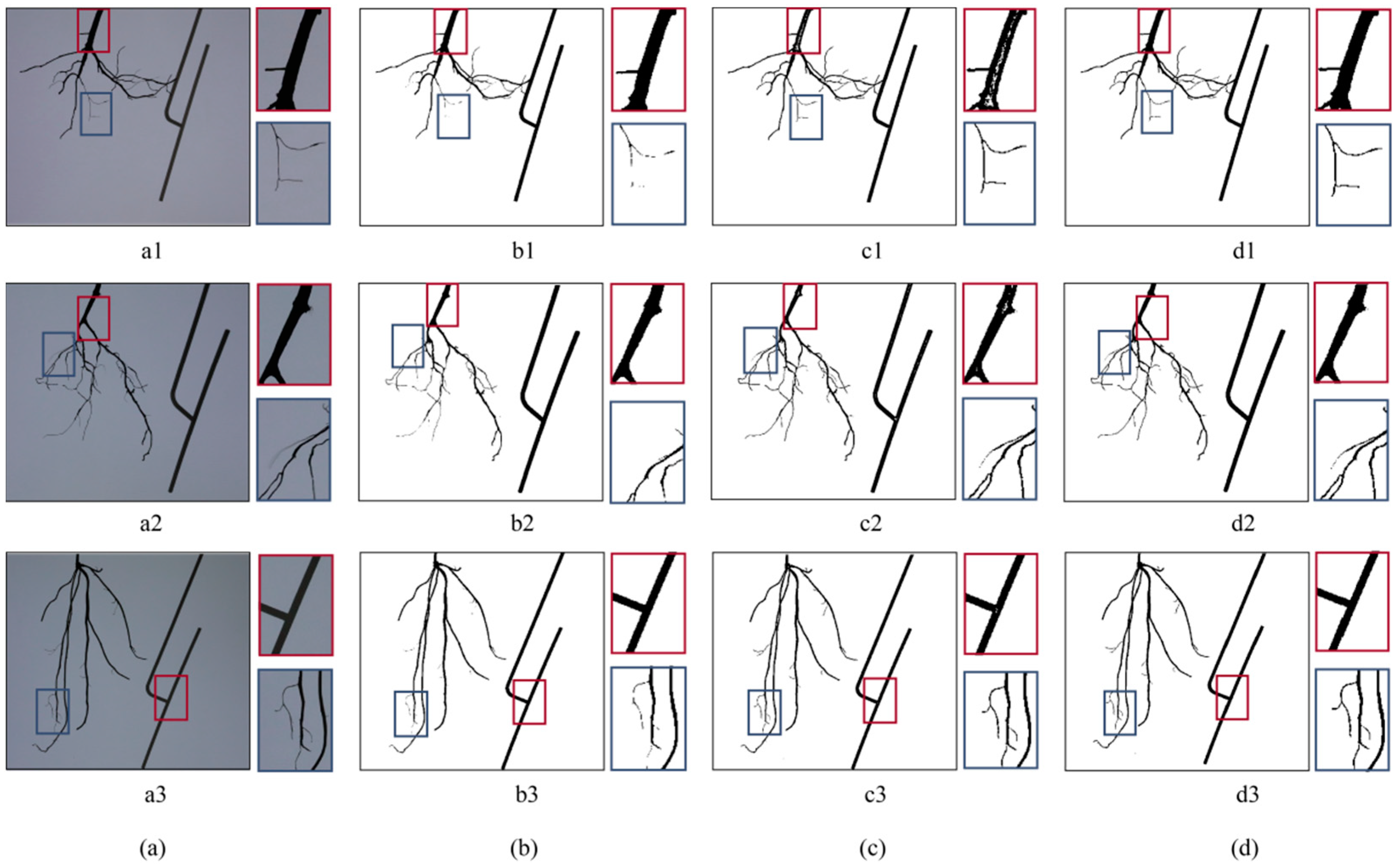
3.1. Segmentation of Target Object

The segmentation results for the original images using different methods are shown in Figure 10. As shown in Figure 10b, with the root systems with many fibrous roots, or in the case of slight vibration during image acquisition, the contrast between the target object and the background was low, significantly affecting the segmentation performance of OTSU, leading to numerous missing areas. The box filter segmentation only applied block filter to process the image. However, because the root diameters varied among different samples, the results could differ based on the size of the block filter. If the size was too small, it could lead to holes in the target area, as shown in Figure 10c. Conversely, if the size was too large, fibrous roots might not be segmented effectively. OTSU-based adaptive threshold segmentation was able to address these issues, making sure that there are no holes in thick root areas, and the fine roots could be correctly segmented. This resulted in the best segmentation performance, as shown in Figure 10d.

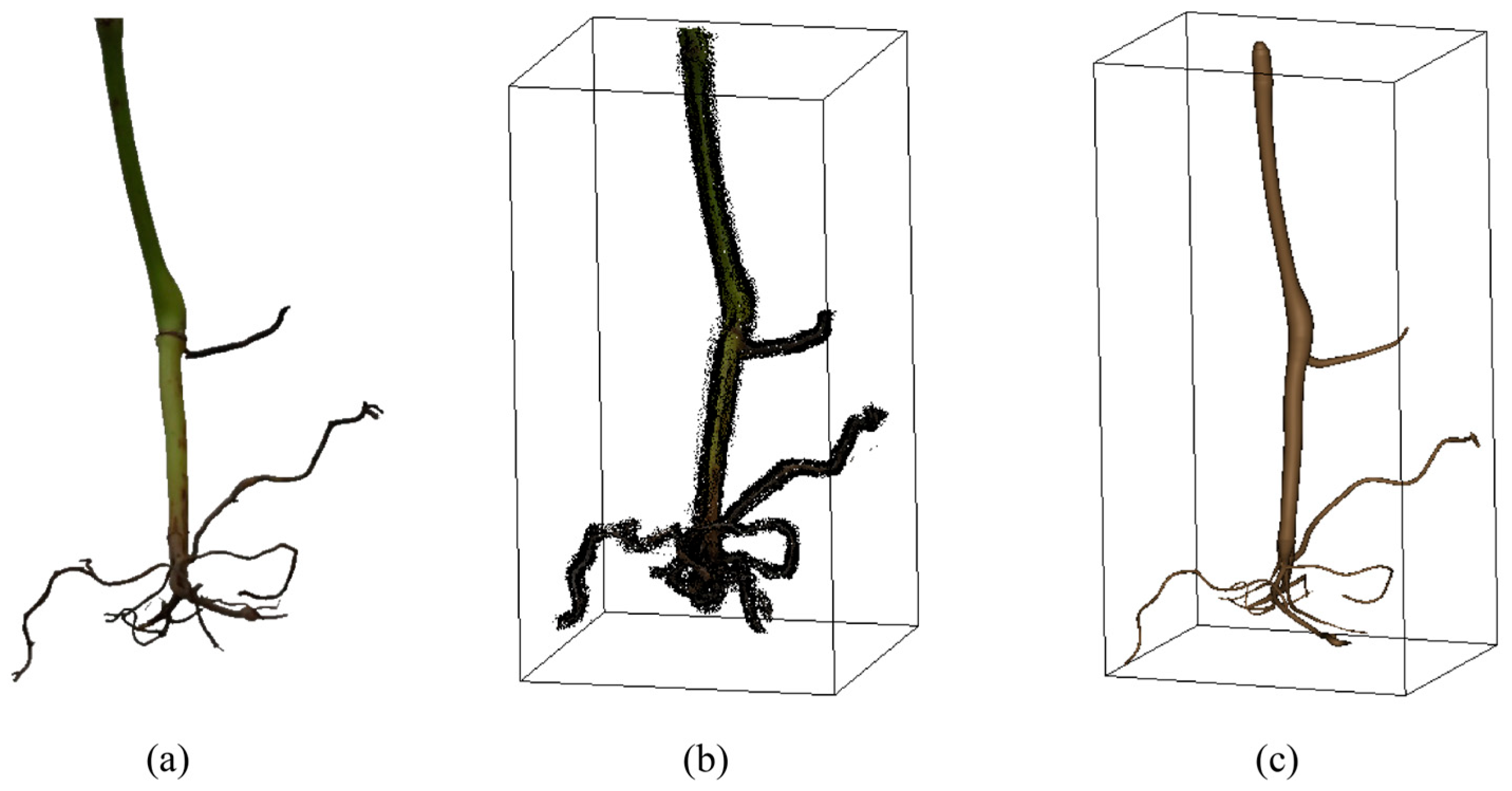
3.2. Three-Dimensional Reconstruction Results

Figure 11 shows the results of skeleton and surface reconstruction. At the same time, current mainstream reconstruction methods, such as Agisoft Metashape, were unable to complete root reconstruction in the tested datasets. This was due to the lack of feature points, which led to the failure of image matching. In Figure 11a, RGB images of three species of root systems were displayed, including Ocimum basilicum (Figure 11(a1)), Sarcandra glabra (Figure 11(a2)), and Sculellaria barbata (Figure 11(a3)). Figure 11(b) presents the results of the skeleton reconstruction, consisting of a uniformly distributed set of points and connecting lines. The skeleton model could also intuitively reflect the morphological characteristics of the root system, and well represent the geometric characteristics of the root system. Compared to other reconstruction algorithms that only provide surface models [28,29], the skeleton model facilitated the calculation of phenotypic parameters such as root number and root length. The smoothing applied during the reconstruction process enhanced the algorithm’s robustness against disturbances, although it sacrificed some bend details, which did not significantly impact the overall results. Figure 11c illustrates the surface reconstruction results, effectively showing variations in root radius. However, when the contrast in radius between parent and lateral roots was substantial, the radius of lateral roots near the connection with the parent root may occasionally appear larger, though this had a minimal effect on the overall outcome. Additionally, since the input images were binary and the surface reconstruction was based on radii and skeleton curves, color information was lost. This could be improved in future studies by integrating color data from original images [14], employing techniques like texture mapping, using RGB-D cameras to capture both depth and color information, or combining Vid2Curve with Gaussian Splatting.

Figure 12 shows the effect of point completion. The result when one of the connection points was an endpoint and one was not is shown from Figure 12(a1–c1), and the result when both connection points were endpoints is shown from Figure 12(a2–c2). In both cases, the point cloud and the surface could be completed correctly.

To demonstrate the advantage of the proposed method, the proposed method was compared with COLMAP. Because COLMAP relied on color and texture features to achieve reconstruction, its input images preserved the color and texture of the root system. Figure 13 shows that there was significant noise in the reconstruction by COLMAP. And the FPE of COLMAP was 1.314 pixels, which was larger than the proposed method (0.544 pixels). Meanwhile, the whole process using COLMAP took about 1 h, while the proposed method only took 2 min.

3.3. Reconstruction Quality

3.3.1. Reconstruction Performance

In this study, a total of 30 seedling roots were used in the reconstruction experiment, including 9 Ob roots, 13 Sg roots, and 8 Sb roots.

Table 1. Projection error of reconstruction of three species’ root systems.

Species	SPE		FPE
	AVG (Pixels)	SD (Pixels)	AVG (Pixels)	SD (Pixels)
Ob	0.588	0.079	0.480	0.029
Sg	0.585	0.109	0.472	0.041
Sb	0.532	0.052	0.451	0.020
Total	0.570	0.090	0.468	0.034

describes the average and the standard deviation of three root system species’ reconstruction results’ projection errors. The SPE and FPE of the reconstructions of the three root species were all less than 0.6 pixels, and the standard deviation was also less than 0.2 pixels, indicating high reconstruction accuracy and good stability.

3.3.2. Phenotypic Parameter Measurement Performance

Table 2. Performance of phenotypic parameter measurements.

Species	Root Number		Root Length
	Precision	Recall	MAE (cm)	MAPE	RMSE (cm)
Ob	0.95	0.95	0.71	1.51%	0.92
Sg	0.97	0.96	1.47	3.61%	1.61
Sb	0.97	0.96	0.90	1.66%	1.37
Total	0.97	0.96	1.06	2.38%	1.35

describes the performance of root number and root length measurement with 26 samples. The root number of the samples ranged from 10 to 27, and the precision and recall of the root number measurement of the reconstruction results achieved 0.97 and 0.96. Nearly one-third of the root number measurement results achieved a precision of 1 and a recall of 1, and FN and PN of other measurement results also did not exceed 2. The root length of the samples ranged from 27.90 cm to 67.50 cm, and the measurement results of all samples achieved an MAE of 1.06 cm, an MAPE of 2.38%, and an RMSE of 1.35 cm. Figure 14 shows the relationship between the measured root length and ground truth for each sample. The calculated R² between predicted values and ground truth values was 0.99 for Ob, 0.99 for Sg, 0.96 for Sb, and 0.99 for all samples, while [41] achieved an R² of 0.92 and [28] achieved an R² of 0.92. The parameters measured from 3D reconstruction results showed high accuracy when compared to the relative manual measurements. It was found in the experiment’s results that self-occlusion of the root system was still the main cause of error. This could be improved in future studies by using the adaptive data acquisition method, to obtain more details from the root system to improve reconstruction results.

3.4. Reconstruction Time Cost

Table 3. Time cost of each procedure.

	AVG	MAX	SD
Image capture	14.07 s	23.00 s	3.30 s
Image preprocessing	13.50 s	16.63 s	1.36 s
3D reconstruction	1.93 min	3.56 min	0.46 min

shows the time cost of each procedure of the proposed reconstruction process in this study. The reconstruction process was divided into three stages: image acquisition, image preprocessing, and 3D reconstruction. The number of input images ranged from 150 to 250, and the average time taken to capture these images was 14.03 s. The maximum time for image preprocessing was less than 17 s, and the length mainly depended on the number of images. The time for 3D reconstruction was the longest, relatively, with an average of 1.93 min and a maximum of 3.56 min, mainly depending on the number of images. The whole process took a maximum of 4.07 min. The short time taken by this method was mainly due to the downsampling of the image, and the iterative process mainly utilizing binary images processed by thinning methods. To improve reconstruction accuracy while ensuring low reconstruction time cost, research will be conducted in the future to reduce the time cost of high-resolution image reconstruction.

4. Conclusions

This study builds a multi-view 3D reconstruction experimental system for root phenotyping. For segmenting root systems from the background of original images, an OTSU-based adaptive threshold segmentation method is proposed. The skeleton-based 3D reconstruction method Vid2Curve is adopted for 3D root system reconstruction. Additionally, a small-size point completion method is proposed for point completion. The 3D reconstruction results showed high quality results, with an average skeleton projection error of 0.570 pixels and an average surface projection error of 0.468 pixels. For phenotypic parameters measurement, this study designs a calibration objection with a thin structure, and proposes a method based on DBSCAN and RANSAC to calculate the scaling factor. The root length and root number measurements achieved high accuracies. Meanwhile, because the images used in the 3D reconstruction process were thinned binary images without color or texture information, the entire process took a very short time, with a maximum time of 4.07 min.

Future research will focus on the improvement of hardware devices and algorithms. The current state of the image acquisition system still requires further refinement, such as in terms of achieving nondestructive image acquisition and collecting images of roots in different growth stages. The reconstruction algorithm will also be improved to realize the reconstruction using high-resolution images to improve accuracy and ensure that the reconstruction speed is still very fast. Moreover, techniques like texture mapping will also be used to reconstruct color information.

References

- Uga, Y.; Sugimoto, K.; Ogawa, S.; Rane, J.; Ishitani, M.; Hara, N.; Kitomi, Y.; Inukai, Y.; Ono, K.; Kanno, N.; et al. Control of root system architecture by DEEPER ROOTING 1 increases rice yield under drought conditions. Nat. Genet. 2013, 45, 1097. [Google Scholar] [CrossRef] [PubMed]
- Mahanta, D.; Rai, R.K.; Mishra, S.D.; Raja, A.; Purakayastha, T.J.; Varghese, E. Influence of phosphorus and biofertilizers on soybean and wheat root growth and properties. Field Crops Res. 2014, 166, 1–9. [Google Scholar] [CrossRef]
- Bonato, T.; Beggio, G.; Pivato, A.; Piazza, R. Maize plant (Zea mays) uptake of organophosphorus and novel brominated flame retardants from hydroponic cultures. Chemosphere 2022, 287, 132456. [Google Scholar] [CrossRef] [PubMed]
- Alemu, A.; Feyissa, T.; Maccaferri, M.; Sciara, G.; Tuberosa, R.; Ammar, K.; Badebo, A.; Acevedo, M.; Letta, T.; Abeyo, B. Genome-wide association analysis unveils novel QTLs for seminal root system architecture traits in Ethiopian durum wheat. BMC Genom. 2021, 22, 20. [Google Scholar] [CrossRef]
- Mathieu, L.; Lobet, G.; Tocquin, P.; Perilleux, C. “Rhizoponics”: A novel hydroponic rhizotron for root system analyses on mature Arabidopsis thaliana plants. Plant Methods 2015, 11, 3. [Google Scholar] [CrossRef] [PubMed]
- Shi, R.; Junker, A.; Seiler, C.; Altmann, T. Phenotyping roots in darkness: Disturbance-free root imaging with near infrared illumination. Funct. Plant Biol. 2018, 45, 400–411. [Google Scholar] [CrossRef] [PubMed]
- Goclawski, J.; Sekulska-Nalewajko, J.; Gajewska, E.; Wielanek, M. An automatic segmentation method for scanned images of wheat root systems with dark discolourations. Int. J. Appl. Math. Comput. Sci. 2009, 19, 679–689. [Google Scholar] [CrossRef]
- Yugan, C.; Xuecheng, Z. Plant root image processing and analysis based on 2D scanner. In Proceedings of the 2010 IEEE Fifth International Conference on Bio-Inspired Computing: Theories and Applications (BIC-TA), Changsha, China, 23–26 September 2010; pp. 1216–1220. [Google Scholar]
- Arnold, T.; Bodner, G. Study of visible imaging and near-infrared imaging spectroscopy for plant root phenotyping. In Proceedings of the Conference on Sensing for Agriculture and Food Quality and Safety X, Orlando, FL, USA, 17–18 April 2018. [Google Scholar]
- Narisetti, N.; Henke, M.; Seiler, C.; Junker, A.; Ostermann, J.; Altmann, T.; Gladilin, E. Fully-automated root image analysis (faRIA). Sci. Rep. 2021, 11, 16047. [Google Scholar] [CrossRef]
- Smith, A.G.; Petersen, J.; Selvan, R.; Rasmussen, C.R. Segmentation of roots in soil with U-Net. Plant Methods 2020, 16, 13. [Google Scholar] [CrossRef]
- Gong, L.; Du, X.; Zhu, K.; Lin, C.; Lin, K.; Wang, T.; Lou, Q.; Yuan, Z.; Huang, G.; Liu, C. Pixel level segmentation of early-stage in-bag rice root for its architecture analysis. Comput. Electron. Agric. 2021, 186, 106197. [Google Scholar] [CrossRef]
- Thesma, V.; Mohammadpour Velni, J. Plant Root Phenotyping Using Deep Conditional GANs and Binary Semantic Segmentation. Sensors 2023, 23, 309. [Google Scholar] [CrossRef] [PubMed]
- Huang, T.; Bian, Y.; Niu, Z.; Taha, M.F.; He, Y.; Qiu, Z. Fast neural distance field-based three-dimensional reconstruction method for geometrical parameter extraction of walnut shell from multiview images. Comput. Electron. Agric. 2024, 224, 109189. [Google Scholar] [CrossRef]
- Zhou, L.; Jin, S.; Wang, J.; Zhang, H.; Shi, M.; Zhou, H. 3D positioning of Camellia oleifera fruit-grabbing points for robotic harvesting. Biosyst. Eng. 2024, 246, 110–121. [Google Scholar] [CrossRef]
- Gregory, P.J.; Hutchison, D.J.; Read, D.B.; Jenneson, P.M.; Gilboy, W.B.; Morton, E.J. Non-invasive imaging of roots with high resolution X-ray micro-tomography. Plant Soil 2003, 255, 351–359. [Google Scholar] [CrossRef]
- Hou, L.; Gao, W.; der Bom van, F.; Weng, Z.; Doolette, C.L.; Maksimenko, A.; Hausermann, D.; Zheng, Y.; Tang, C.; Lombi, E.; et al. Use of X-ray tomography for examining root architecture in soils. Geoderma 2022, 405, 115405. [Google Scholar] [CrossRef]
- Jiang, Z.; Leung, A.K.; Liu, J. Segmentation uncertainty of vegetated porous media propagates during X-ray CT image-based analysis. Plant Soil 2024. [Google Scholar] [CrossRef]
- Metzner, R.; Eggert, A.; van Dusschoten, D.; Pflugfelder, D.; Gerth, S.; Schurr, U.; Uhlmann, N.; Jahnke, S. Direct comparison of MRI and X-ray CT technologies for 3D imaging of root systems in soil: Potential and challenges for root trait quantification. Plant Methods 2015, 11, 17. [Google Scholar] [CrossRef] [PubMed]
- van Dusschoten, D.; Metzner, R.; Kochs, J.; Postma, J.A.; Pflugfelder, D.; Buehler, J.; Schurr, U.; Jahnke, S. Quantitative 3D Analysis of Plant Roots Growing in Soil Using Magnetic Resonance Imaging. Plant Physiol. 2016, 170, 1176–1188. [Google Scholar] [CrossRef]
- Heeren, B.; Paulus, S.; Goldbach, H.; Kuhlmann, H.; Mahlein, A.-K.; Rumpf, M.; Wirth, B. Statistical shape analysis of tap roots: A methodological case study on laser scanned sugar beets. BMC Bioinform. 2020, 21, 335. [Google Scholar] [CrossRef]
- Todo, C.; Ikeno, H.; Yamase, K.; Tanikawa, T.; Ohashi, M.; Dannoura, M.; Kimura, T.; Hirano, Y. Reconstruction of Conifer Root Systems Mapped with Point Cloud Data Obtained by 3D Laser Scanning Compared with Manual Measurement. Forests 2021, 12, 1117. [Google Scholar] [CrossRef]
- Kargar, A.R.; MacKenzie, R.A.; Apwong, M.; Hughes, E.; van Aardt, J. Stem and root assessment in mangrove forests using a low-cost, rapid-scan terrestrial laser scanner. Wetl. Ecol. Manag. 2020, 28, 883–900. [Google Scholar] [CrossRef]
- Pflugfelder, D.; Kochs, J.; Koller, R.; Jahnke, S.; Mohl, C.; Pariyar, S.; Fassbender, H.; Nagel, K.A.; Watt, M.; van Dusschoten, D.; et al. The root system architecture of wheat establishing in soil is associated with varying elongation rates of seminal roots: Quantification using 4D magnetic resonance imaging. J. Exp. Bot. 2022, 73, 2050–2060. [Google Scholar] [CrossRef] [PubMed]
- Schneider, H.M.; Postma, J.A.; Kochs, J.; Pflugfelder, D.; Lynch, J.P.; van Dusschoten, D. Spatio-Temporal Variation in Water Uptake in Seminal and Nodal Root Systems of Barley Plants Grown in Soil. Front. Plant Sci. 2020, 11, 1247. [Google Scholar] [CrossRef] [PubMed]
- Feng, L.; Chen, S.; Wu, B.; Liu, Y.; Tang, W.; Liu, F.; He, Y.; Zhang, C. Detection of oilseed rape clubroot based on low-field nuclear magnetic resonance imaging. Comput. Electron. Agric. 2024, 218, 108687. [Google Scholar] [CrossRef]
- Wu, Q.; Wu, J.; Hu, P.; Zhang, W.; Ma, Y.; Yu, K.; Guo, Y.; Cao, J.; Li, H.; Li, B.; et al. Quantification of the three-dimensional root system architecture using an automated rotating imaging system. Plant Methods 2023, 19, 11. [Google Scholar] [CrossRef]
- Sunvittayakul, P.; Kittipadakul, P.; Wonnapinij, P.; Chanchay, P.; Wannitikul, P.; Sathitnaitham, S.; Phanthanong, P.; Changwitchukarn, K.; Suttangkakul, A.; Ceballos, H.; et al. Cassava root crown phenotyping using three-dimension (3D) multi-view stereo reconstruction. Sci. Rep. 2022, 12, 10030. [Google Scholar] [CrossRef] [PubMed]
- Lu, Y.; Wang, Y.; Parikh, D.; Khan, A.; Lu, G. Simultaneous Direct Depth Estimation and Synthesis Stereo for Single Image Plant Root Reconstruction. IEEE Trans. Image Process. 2021, 30, 4883–4893. [Google Scholar] [CrossRef]
- Masuda, T. 3D Shape Reconstruction of Plant Roots in a Cylindrical Tank From Multiview Images. In Proceedings of the IEEE/CVF International Conference on Computer Vision (ICCV), Seoul, Republic of Korea, 27 October–2 November 2019; pp. 2149–2157. [Google Scholar]
- Liu, L.; Chen, N.; Ceylan, D.; Theobalt, C.; Wang, W.; Mitra, N.J.; Assoc Comp, M. CURVEFUSION: Reconstructing Thin Structures from RGBD Sequences. In Proceedings of the 11th ACM SIGGRAPH Conference and Exhibition on Computer Graphics and Interactive Techniques in Asia (SA), Tokyo, Japan, 4–7 December 2018. [Google Scholar]
- Martin, T.; Montes, J.; Bazin, J.-C.; Popa, T. Topology-aware reconstruction of thin tubular structures. In Proceedings of the SIGGRAPH Asia 2014 Technical Briefs, Shenzhen, China, 3–6 December 2014; p. 12. [Google Scholar]
- Li, S.; Yao, Y.; Fang, T.; Quan, L. Reconstructing Thin Structures of Manifold Surfaces by Integrating Spatial Curves. In Proceedings of the 31st IEEE/CVF Conference on Computer Vision and Pattern Recognition (CVPR), Salt Lake City, UT, USA, 18–23 June 2018; pp. 2887–2896. [Google Scholar]
- Tabb, A. Shape from Silhouette Probability Maps: Reconstruction of thin objects in the presence of silhouette extraction and calibration error. In Proceedings of the 26th IEEE Conference on Computer Vision and Pattern Recognition (CVPR), Portland, OR, USA, 23–28 June 2013; pp. 161–168. [Google Scholar]
- Tabb, A.; Medeiros, H. A robotic vision system to measure tree traits. In Proceedings of the 2017 IEEE/RSJ International Conference on Intelligent Robots and Systems (IROS), 24–28 September 2017; pp. 6005–6012. [Google Scholar]
- Wang, P.; Liu, L.; Chen, N.; Chu, H.-K.; Theobalt, C.; Wang, W. Vid2Curve: Simultaneous Camera Motion Estimation and Thin Structure Reconstruction from an RGB Video. ACM Trans. Graph. 2020, 39, 132-1. [Google Scholar] [CrossRef]
- Otsu, N. A Threshold Selection Method from Gray-Level Histograms. IEEE Trans. Syst. Man Cybern. 1979, 9, 62–66. [Google Scholar] [CrossRef]
- Olson, E. AprilTag: A robust and flexible visual fiducial system. In Proceedings of the IEEE International Conference on Robotics and Automation (ICRA), Shanghai, China, 9–13 May 2011. [Google Scholar]
- Ester, M.; Kriegel, H.-P.; Sander, J.; Xu, X. A Density-Based Algorithm for Discovering Clusters in Large Spatial Databases with Noise. In Proceedings of the Knowledge Discovery and Data Mining, Portland, OR, USA, 2–4 August 1996. [Google Scholar]
- Fischler, M.A.; Bolles, R.C. Random sample consensus: A paradigm for model fitting with applications to image analysis and automated cartography. Commun. ACM 1981, 24, 381–395. [Google Scholar] [CrossRef]
- Okamoto, Y.; Ikeno, H.; Hirano, Y.; Tanikawa, T.; Yamase, K.; Todo, C.; Dannoura, M.; Ohashi, M. 3D reconstruction using Structure-from-Motion: A new technique for morphological measurement of tree root systems. Plant Soil 2022, 477, 829–841. [Google Scholar] [CrossRef]