Research on Flexible Job Shop Scheduling Method for Agricultural Equipment Considering Multi-Resource Constraints


Abstract
1. Introduction
2. Materials and Methods
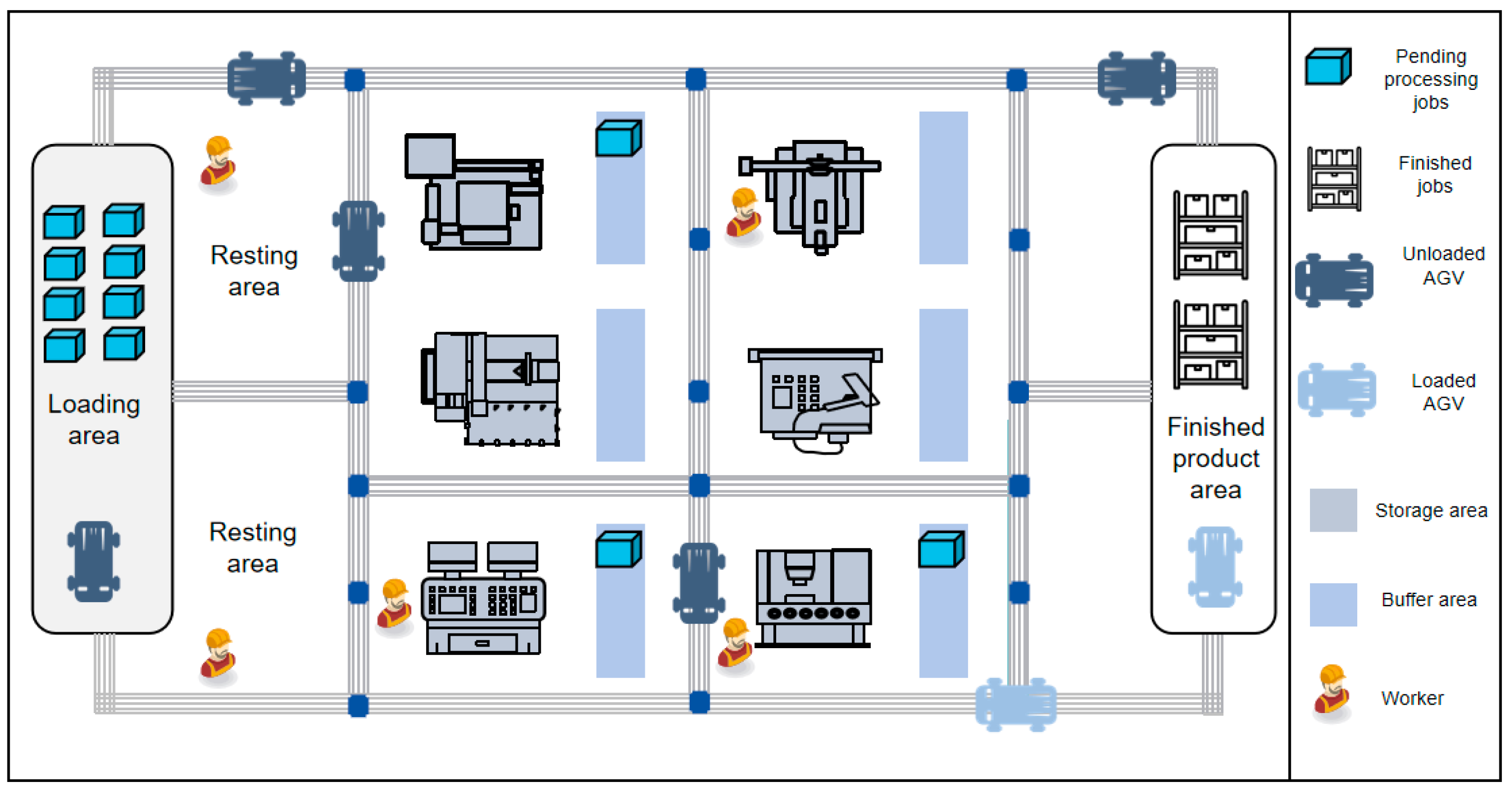
2.1. Problem Description
- (1)
- Jobs and Operations
- (2)
- Machines
- (3)
- Workers
- (4)
- AGVs
- (1)
- Machine Allocation: Assign each operation to a machine that can process it.
- (2)
- Worker Allocation: Assign each operation to a worker who can operate the selected machine.
- (3)
- AGV Allocation: Assign each job to an AGV for transportation to the designated machine.
- (4)
- Operation Sequence: Determine the order in which operations are processed on each machine.
- (5)
- Transportation Sequence: Determine the order in which AGVs transport jobs between the LU area and machines.
- (1)
- Minimize Makespan: The maximum completion time of all jobs.
- (2)
- Minimize Maximum Continuous Working Hours of Workers: The longest continuous working period for any worker.
- (1)
- Each machine can process at most one operation at a time.
- (2)
- A worker can only operate one machine at a time.
- (3)
- Only one machine can be selected for each operation and one AVG can be selected for job Ji before operation Oij, and they cannot be interrupted during processing.
- (4)
- All the jobs, machines, and workers are available at zero time. All the jobs and AGVs are located in the loading/unloading(LU) area at zero time.
- (5)
- The processing operations for the same job shall meet the constraints of the operation sequence.
- (6)
- Disregarding the transfer time of workers between machines, a worker can only operate one machine at a time.
- (7)
- Machine and AVG failures are not considered and the AVGs are sufficiently charged, and the loading and unloading time of the material on the machine is not considered.
- (8)
- An AVG can only load one job at a time.
- (9)
- After the current transportation task is completed, the AGV will not return to the loading and unloading area, but will go to the machine where the next transportation task is to be performed.
- (10)
- Each machine has a buffer zone that can be used to park AGVs and store operations with sufficient buffer capacity.
2.2. Mathematical Model
2.3. Grey Wolf Optimization Algorithm
2.4. Multi-Object Discrete Grey Wolf Optimization Algorithm for MRCFJSP
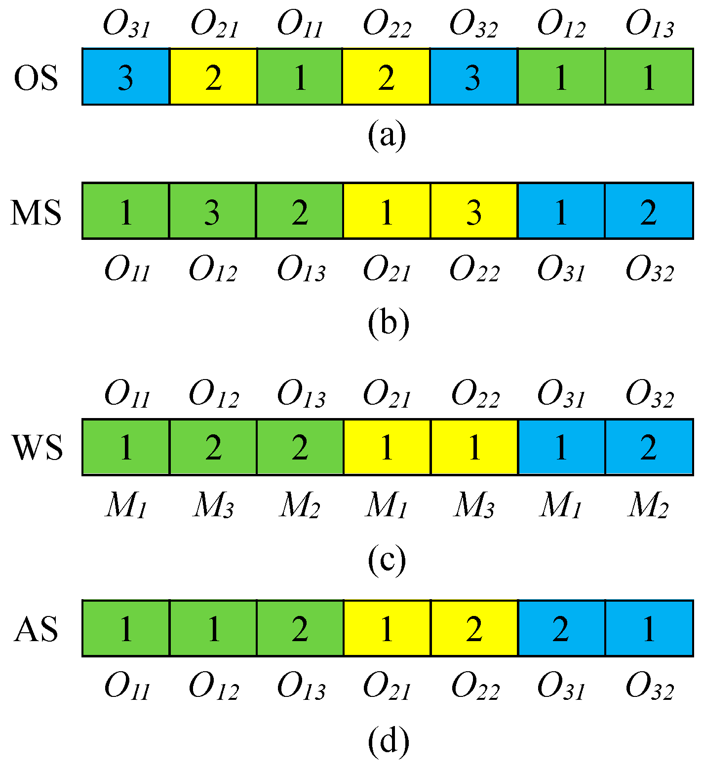
2.4.1. Four-Vector Encoding
- (1)
- Operation sequence vector
- (2)
- Machine selection vector
- (3)
- Worker selection vector and AGV selection vector
2.4.2. Decoding
2.4.3. Population Initialization
- (1)
- Most work remaining rule [27]: The job that has the maximum total processing time remaining is prioritized for execution first.
- (2)
- Most number of operations remaining rule [26]: The job that has the most remaining operations is processed first.
- (3)
- Random rule: Operation sequencing is randomly generated.
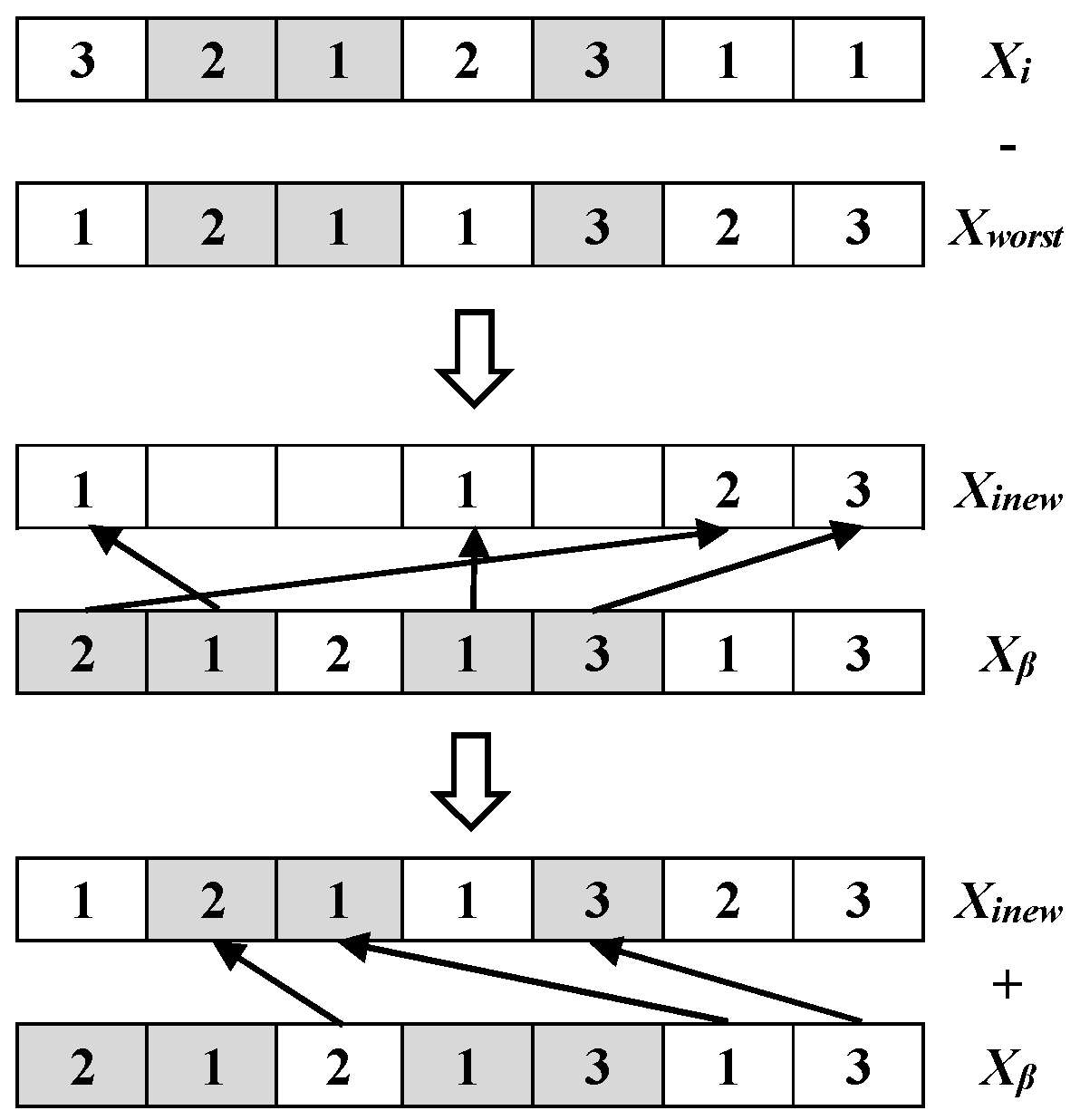
2.4.4. Solution-Updating Mechanism
- (1)
- Operation sequencing
- Step 1. Identify the worst individual (Xworst) and choose one form Xα, Xβ, and Xδ randomly as Xbest (assuming that Xβ is selected) from the population.
- Step2. Identify similar assignments of operations in the individual Xi and Xworst.
- Step 3. Eliminate similar assignments from Xi and transfer the remaining assignments to a new solution Xinew.
- Step 4. Beginning from the initial assignment of Xβ, eliminate the assignments corresponding to the remaining assignments of individual Xinew.
- Step 5. Beginning from the initial assignment of Xβ, transfer the remaining assignments of Xβ in the vacant elements of individual Xinew in the corresponding order.
- (2)
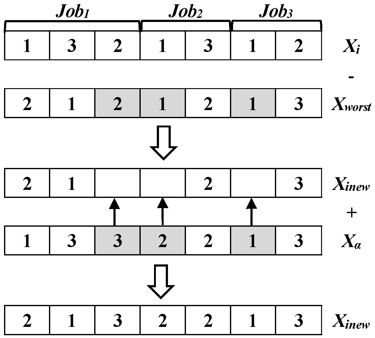
- Machine selection and AGV selection
- Step 1. Identify the best individual Xbest (Assuming it is Xα) and worst individual Xworst from the population.
- Step 2. Identify similar assignments of machines assigned to the same machines in the individuals Xi and Xworst.
- Step 3. Eliminate similar assignments from the individual Xi and transfer the remaining assignments to a new solution Xinew.
- Step 4. Transfer the corresponding machine assignments of Xα to the vacant elements of individual Xinew.
- (3)
- Worker selection
2.4.5. Local Search
- (1)
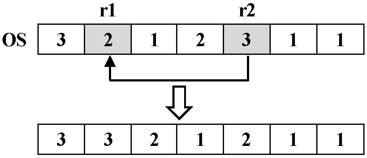
- VNS1 (Insert, for OS vectors): Within the length range of the OS vector, randomly generate two positions r1 and r2 (r1 < r2), insert the element corresponding to r2 into position r1, and move the elements after position r1 backwards in sequence. For the OS vector in Figure 3, the two generated random numbers r1 and r2 are 2 and 5, respectively. The solution process of VNS1 is shown in Figure 6.
- (2)
- VNS2 (Choose the minimum processing time, for MS vectors): Randomly generate r ∈ [1, N] random numbers, where N is the total number of operations, and randomly select r positions from the MS vector. For each selected position corresponding to an operation, select the machine with the shortest processing time from its corresponding optional machine set for replacement. After replacement, check whether the workers corresponding to r positions in WS can operate the newly selected equipment. If it is not feasible, randomly select a worker from the operable worker set of the new equipment. For the solution generated in Figure 7, MS is 1,122,312, and r = 3 is randomly generated. Three positions are randomly selected, such as positions 2, 3, and 7. The solution process of VNS2 is shown in Figure 7.
- (3)
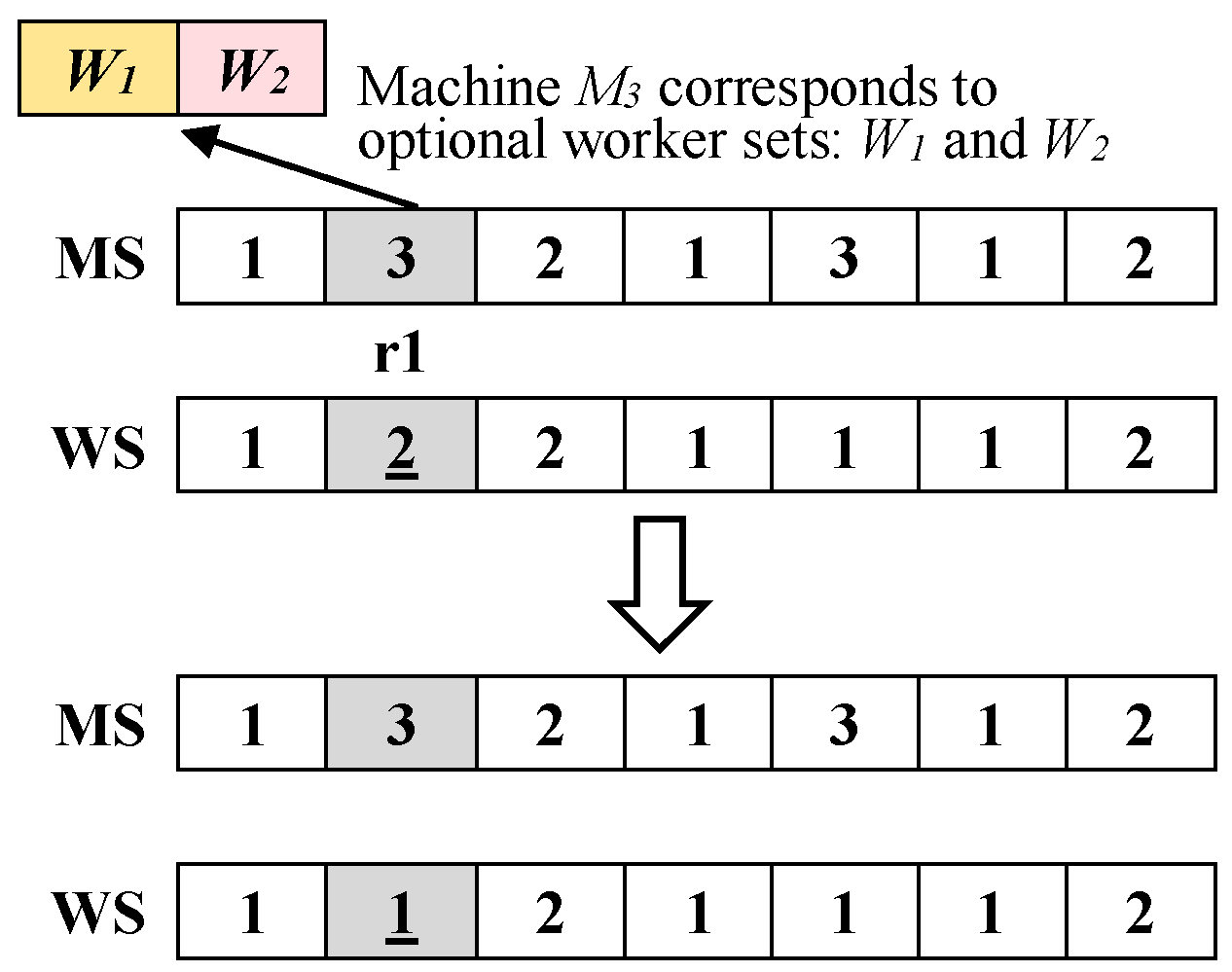
- VNS3 (Flip, for WS vectors): Within the length range of the WS vector, randomly generate a position r1. In the MS vector, position r1 should correspond to more than one available processing worker for the processing equipment, and then select a new worker from the set of available workers for equipment replacement. The solution process of VNS3 is shown in Figure 8. From Figure 8, it can be observed that: Machine M3 can be operated by either workers W1 or W2. Initially, worker W2 was selected for operating machine M3. After VNS3, worker W1 is chosen to operate machine M3 instead.
- (4)
- VNS4 (swap, for AS vectors): Within the length of the AS vector, two randomly generated positions r1 and r2 (r1 ≠ r2) are exchanged for the elements at the r1 and r2 positions. The solution process of VNS4 is shown in Figure 9.
3. Results
3.1. Performance Metrics
- (1)
- Inverse Generational Distance (IGD): Measure the average distance from a predefined set of uniformly spaced points along the true or ideal Pareto front (denoted as PF*) to the nearest solution in the obtained PF. Essentially, IGD assesses how well the obtained solutions approximate the true Pareto front by calculating these distances and averaging them.
- |PF*| is the number of uniformly spaced points along the true Pareto front.
- PF*i represents the ith point in PF*.
- PF is the set of obtained solutions (Pareto front).
- PFj represents the jth solution in PF.
- d(PF*i, PFj) is the Euclidean distance between point PF*i and the closest solution PFj in PF.
- (2)
- Hypervolume (HV): HV is the volume of a hyper polyhedron enclosed by non-dominated solutions and reference points in the search space, calculated as follows:
3.2. Test Instances Generation
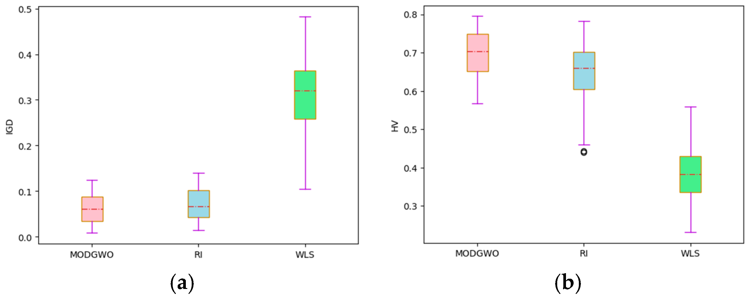
3.3. Effectiveness Verification for a Hybrid Initialization Method
- (1)
- MODGWO represents the method proposed in this paper.
- (2)
- RI (random initialization) indicates that MODGWO uses a random initialization method to obtain the initial solution.
- (3)
- WLS (without local search) indicates that MODGWO does not use a local search procedure, but only a single tracking mode for searching.
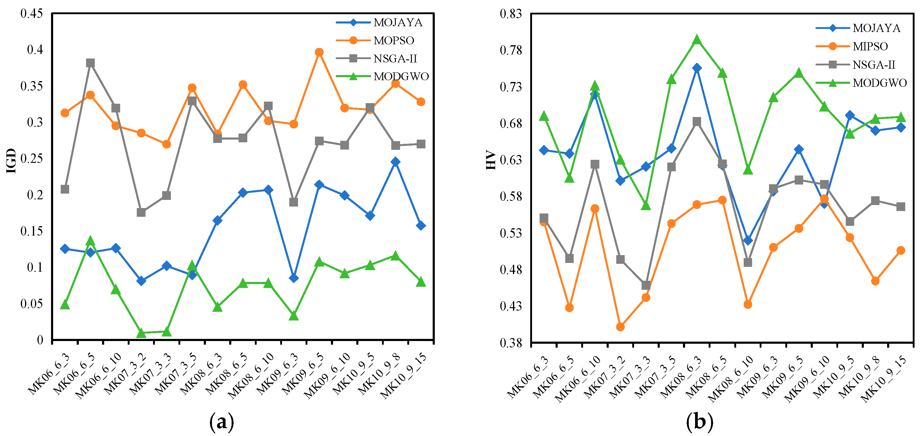
3.4. Comparison with Other Algorithms
3.5. Scheduling Gantt Chart
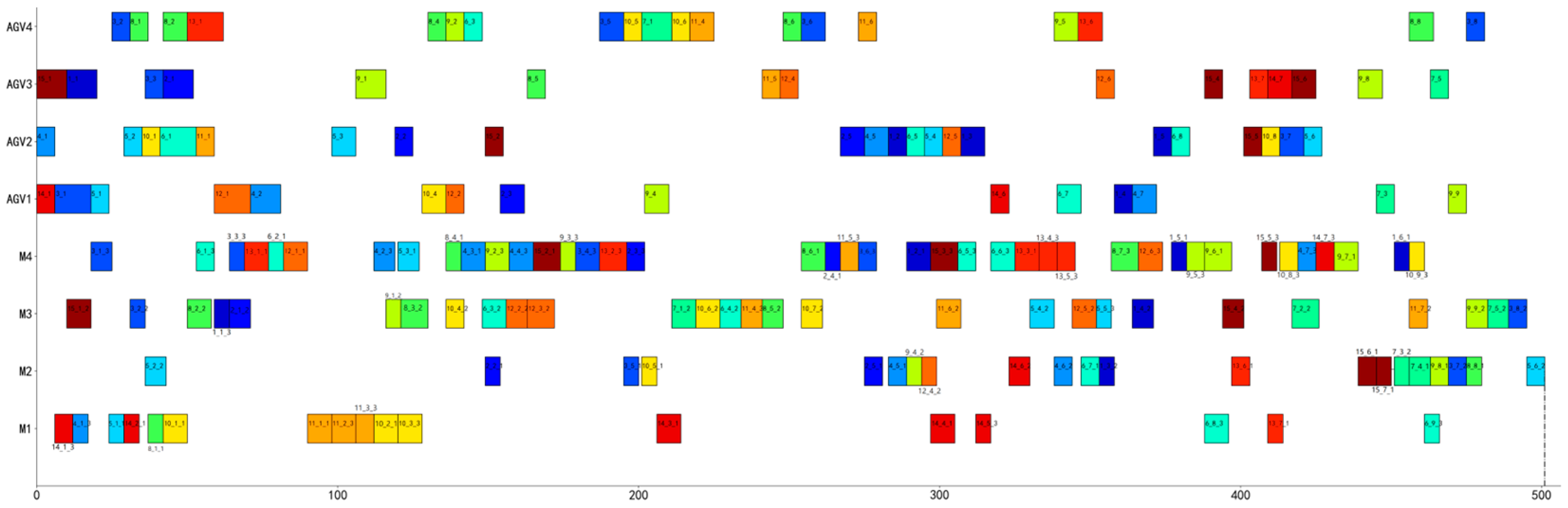
3.6. Examples of Agricultural Machinery and Equipment Production
4. Discussion
5. Conclusions
Author Contributions
Funding
Institutional Review Board Statement
Data Availability Statement
Conflicts of Interest
References
- Huang, Q.H.; He, J. The Core Capability, Function and Strategy of Chinese Manufacturing Industry-Comment on “Chinese Manufacturing 2025”. China Ind. Econ. 2015, 327, 5–17. [Google Scholar]
- Liu, M.Z.; Wang, M.C.; Zhang, M.X. Dynamic just-in-time material distribution system for mixed model assembly lines under uncertainty. Comput. Integr. Manuf. Syst. 2014, 20, 3020–3031. [Google Scholar]
- Brucker, P.; Schlie, R. Job-shop scheduling with multi-purpose machines. Computing 1990, 45, 369–375. [Google Scholar] [CrossRef]
- Mahmoodjanloo, M.; Tavakkoli-moghaddam, R.; Baboli, A.; Bozorgi-Amiri, A. Flexible job shop scheduling problem with reconfigurable machine tools: An improved differential evolution algorithm. Appl. Soft Comput. 2020, 94, 106416. [Google Scholar] [CrossRef]
- Fan, J.; Zhang, C.; Shen, W.; Gao, L. A matheuristic for flexible job shop scheduling problem with lot-streaming and machine reconfigurations. Int. J. Prod. Res. 2023, 61, 6565–6588. [Google Scholar] [CrossRef]
- Guevara, G.; Pereira, A.; Ferreira, A.; Barbosa, J.; Leitão, P. Genetic algorithm for flexible job shop scheduling problem—A case study. AIP Conf. Proc. 2015, 1648, 140006. [Google Scholar]
- Barak, S.; Moghdani, R.; Maghsoudlou, H. Energy-efficient multi-objective flexible manufacturing scheduling. J. Clean. Prod. 2021, 283, 124610. [Google Scholar] [CrossRef]
- Ayyoubzadeh, B.; Ebrahimnejad, S.; Bashiri, M.; Baradaran, V.; Hosseini, S. Modelling and an improved NSGA-II algorithm for sustainable manufacturing systems with energy conservation under environmental uncertainties: A case study. Int. J. Sustain. Eng. 2021, 14, 255–279. [Google Scholar] [CrossRef]
- Xu, J.; Xu, X.; Xie, S.Q. Recent developments in dual resource constrained (DRC) system research. Eur. J. Oper. Res. 2011, 215, 309–318. [Google Scholar] [CrossRef]
- Wu, R.; Li, Y.; Guo, S.; Xu, W. Solving the dual-resource constrained flexible job shop scheduling problem with learning effect by a hybrid genetic algorithm. Adv. Mech. Eng. 2018, 10, 1687814018804096. [Google Scholar] [CrossRef]
- Kress, D.; Müller, D.; Nossack, J. A worker constrained flexible job shop scheduling problem with sequence-dependent setup times. OR Spectr. 2019, 41, 179–217. [Google Scholar] [CrossRef]
- Gong, G.; Deng, Q.; Gong, X.; Liu, W.; Ren, Q. A new double flexible job shop scheduling problem integrating processing time, green production, and human factor indicators. J. Clean. Prod. 2018, 174, 560–576. [Google Scholar] [CrossRef]
- Vital-Soto, A.; Baki, M.F.; Azab, A. A multi-objective mathematical model and evolutionary algorithm for the dual-resource flexible job-shop scheduling problem with sequencing flexibility. Flex. Serv. Manuf. J. 2022, 35, 626–668. [Google Scholar] [CrossRef]
- Raman, N.; Talbot, F.B.; Rachamadugu, R.V. Simultaneous scheduling of machines and material handling devices in automated manufacturing. In Proceedings of the 2nd ORSA/TIMS Conference on FMS: OR Models and Applications, Ann Arbor, MI, USA, 12–15 August 1986. [Google Scholar]
- Yan, J.; Liu, Z.; Zhang, C.; Zhang, T.; Zhang, Y.; Yang, C. Research on flexible job shop scheduling under finite transportation conditions for digital twin workshop. Robot. Comput.-Integr. Manuf. 2021, 72, 102198. [Google Scholar] [CrossRef]
- Hu, H.; Jia, X.; He, Q.; Fu, S.; Liu, K. Deep reinforcement learning based AGVs real-time scheduling with mixed rule for flexible shop floor in Industry 4.0. Comput. Ind. Eng. 2020, 149, 106749. [Google Scholar] [CrossRef]
- Umar, U.A.; Ariffin MK, A.; Ismail, N.; Tang, S. Hybrid multi objective genetic algorithms for integrated dynamic scheduling and routing of jobs and automated-guided vehicle (AGV) in flexible manufacturing systems (FMS) environment. Int. J. Adv. Manuf. Technol. 2015, 81, 2123–2141. [Google Scholar] [CrossRef]
- Tan, W.; Yuan, X.; Huang, G.; Liu, Z. Low-carbon joint scheduling in flexible open-shop environment with constrained automatic guided vehicle by multi-objective particle swarm optimization. Appl. Soft Comput. 2021, 111, 107695. [Google Scholar] [CrossRef]
- Berterottière, L.; Dauzère-Pérès, S.; Yugma, C. Flexible job-shop scheduling with transportation resources. Eur. J. Oper. Res. 2024, 312, 890–909. [Google Scholar] [CrossRef]
- Mirjalili, S.; Mirjalilis, M.; Lewis, A. Grey wolf optimizer. Adv. Eng. Softw. 2014, 69, 46–61. [Google Scholar] [CrossRef]
- Shaheen, M.A.; Hasanien, H.M.; Alkuhayli, A. A novel hybrid GWO-PSO optimization technique for optimal reactive power dispatch problem solution. Ain Shams Eng. J. 2021, 12, 621–630. [Google Scholar] [CrossRef]
- Nadimi-Shahraki, M.H.; Taghian, S.; Mirjalili, S. An improved grey wolf optimizer for solving engineering problems. Expert Syst. Appl. 2021, 166, 113917. [Google Scholar] [CrossRef]
- Li, H.; Lv, T.; Ma, Z.S. An Improved grey wolf optimizer with weighting functions and its application to Unmanned Aerial Vehicles path planning. Comput. Electr. Eng. 2023, 111 Pt A, 108893. [Google Scholar] [CrossRef]
- Liu, X.; Tian, Y.; Lei, X.; Wang, H.; Wang, J. An improved self-adaptive grey wolf optimizer for the daily optimal operation of cascade pumping stations. Appl. Soft Comput. J. 2019, 75, 473–493. [Google Scholar] [CrossRef]
- Ho, N.B.; Tay, J.C. GENACE: An efficient cultural algorithm for solving the flexible job-shop problem. In Proceedings of the 2004 Congress on Evolutionary Computation (IEEE Cat. No. 04TH8753), Portland, OR, USA, 19–23 June 2004; Volume 2, pp. 1759–1766. [Google Scholar]
- Pezzella, F.; Morganti, G.; Ciaschetti, G. A genetic algorithm for the flexible job-shop scheduling problem. Comput. Oper. Res. 2008, 35, 3202–3212. [Google Scholar] [CrossRef]
- Brandimarte, P. Routing and scheduling in a flexible job shop by tabu search. Ann. Oper. Res. 1993, 41, 157–183. [Google Scholar] [CrossRef]
- Kacem, I.; Hammadi, S.; Borne, P. Pareto-optimality approach for flexible jobshop scheduling problems: Hybridization of evolutionary algorithms and fuzzy logic. Math. Comput. Simul. 2014, 60, 245–276. [Google Scholar] [CrossRef]
- Li, J.Q.; Pan, Q.K.; Tasgetiren, M.F. A discrete artificial bee colony algorithm for the multi-objective flexible job-shop scheduling problem with maintenance activities. Appl. Math. Model. 2014, 38, 1111–1132. [Google Scholar] [CrossRef]
- Rao, V.R. Jaya: A simple and new optimization algorithm for solving constrained and unconstrained optimization problems. Int. J. Ind. Eng. Comput. 2016, 7, 19–34. [Google Scholar]
- Rylan, H.; Caldeira, A. Gnanavelbabu. Solving the flexible job shop scheduling problem using an improved Jaya algorithm. Comput. Ind. Eng. 2019, 137, 106064. [Google Scholar]
- Coello, C.A.C.; Cortés, N.C. Solving multiobjective optimization problems using an artificial immune system. Genet. Program. Evolvable Mach. 2005, 6, 163–190. [Google Scholar] [CrossRef]
- Zitzler, E.; Thiele, L. Multiobjective evolutionary algorithms: A comparative case study and the strength pareto approach. IEEE Trans. Evol. Comput. 1999, 3, 257–271. [Google Scholar] [CrossRef]
- Zhang, S.; Du, H.; Borucki, S.; Jin, S.; Hou, T.; Li, Z. Dual resource constrained flexible job shop scheduling based on improved quantum genetic algorithm. Machines 2021, 9, 108. [Google Scholar] [CrossRef]
- Rinaldi, M.; Fera, M.; Bottani, E.; Grosse, E.H. Workforce scheduling incorporating worker skills and ergonomic constraints. Comput. Ind. Eng. 2022, 168, 108107. [Google Scholar] [CrossRef]
- Homayouni, S.M.; Fontes, D.B.M.M. Production and transport scheduling in flexible job shop manufacturing systems. J. Glob. Optim. 2021, 79, 463–502. [Google Scholar] [CrossRef]
- Reddy, N.S.; Ramamurthy, D.V.; Padma Lalitha, M.; Prahlada Rao, K. Integrated simultaneous scheduling of machines automated guided vehicles and tools in multi machine flexible manufacturing system using symbiotic organisms search algorithm. J. Ind. Prod. Eng. 2022, 39, 317–339. [Google Scholar] [CrossRef]
- Jing, Z.; Wang, W.; Xu, X. A hybrid discrete particle swarm optimization for dual-resource constrained job shop scheduling with resource flexibility. J. Intell. Manuf. 2017, 28, 1961–1972. [Google Scholar]
- Rylan, H.; Caldeira, A.; Gnanavelbabu, A. Pareto based discrete Jaya algorithm for multi-objective flexible job shop scheduling problem. Expert Syst. Appl. 2021, 170, 11567. [Google Scholar]
- Ulusoy, G.; Bilge, Ü. Simultaneous scheduling of machines and automated guided vehicles. Int. J. Prod. Res. 1993, 31, 2857–2873. [Google Scholar] [CrossRef]


| Notation | Description |
|---|---|
| Indexes and set | |
| i, i′, h | index of jobs, i, i′, h ∈ {1, 2,…, n} |
| j, j′, g | index of operations, j, j′, g ∈ {1, 2,…, ri} |
| k, q | index of machines, k, q ∈ {1, 2,…, m} |
| s, r | index of workers, s, r ∈ {1, 2,…, l} |
| v | index of AVGs, v ∈ {1, 2,…, w} |
| Ji | The ith job |
| Mk | The kth machine |
| Ws | The sth worker |
| Av | The vth AVG |
| Oij | The jth operation of Ji |
| Ωij | The set of compatible machines of Oij |
| λk | The set of compatible workers of Mk |
| Parameters | |
| n | Number of total jobs |
| ri | Number of operations of Ji |
| m | Number of total machines |
| l | Number of total workers |
| w | Number of total AVGs |
| Pijks | The processing time of Oij on Mk operated by Ws |
| STij | The start time of Oij |
| CTij | The completion time of Oij |
| Ci | The completion time of the last operation of Ji |
| STijv | The start time of AGV Vv when transporting Oij |
| CTijv | The completion time of AGV Vv when transporting Oij |
| tgk | Delivery time of AGV Vv from machine Mg to machine Mk |
| Ts | Maximum continuous working hours for worker Ws |
| L | a sufficiently large positive integer |
| Decision variables | |
| xijk | a binary variable: if Oij is assigned on Mk, xijk = 1, otherwise xijk = 0 |
| xijks | a binary variable: if Oij is assigned on Mk operated by Ws, xijks = 1, otherwise xijks = 0 |
| yiji′j′ks | a binary variable: if Oij is ahead of Oi′j′ assigned on Mk operated by Ws, yiji′j′ks = 1, otherwise yiji′j′ks = 0 |
| ziji′j′k | a binary variable: if Oij is ahead of Oi′j′ assigned on Mk, ziji′j′k = 1, otherwise ziji′j′k = 0 |
| αijv | a binary variable: if Oij is transported by AVG Vv, αijv = 1, otherwise αijv = 0 |
| βiji′j′v | a binary variable: if Oij is ahead of Oi′j′ transported by AVG Vv, βiji′j′v = 1, otherwise βiji′j′v = 0 |
| Job | Operation | Processing Time | ||
|---|---|---|---|---|
| M1 | M2 | M3 | ||
| J1 | O11 | 2 | 3 | - |
| O12 | 2 | - | 1 | |
| O13 | 3 | 4 | 3 | |
| J2 | O21 | 1 | 3 | - |
| O22 | - | 2 | 2 | |
| J3 | O31 | 5 | - | 7 |
| O32 | - | 8 | 6 | |
| W1 | W2 | |
|---|---|---|
| M1 | √ | - |
| M2 | - | √ |
| M3 | √ | √ |
| Instance ID | Scale (n × m) | Number of Workers | Number of AVGs |
|---|---|---|---|
| MK01 | 10 × 6 | 4 | 2, 3, 6 |
| MK02 | 10 × 6 | 4 | 2, 3, 6 |
| MK03 | 15 × 8 | 5 | 3, 4, 8 |
| MK04 | 15 × 8 | 5 | 3, 4, 8 |
| MK05 | 15 × 4 | 3 | 1, 2, 4 |
| MK06 | 10 × 10 | 6 | 3, 5, 10 |
| MK07 | 20 × 5 | 3 | 2, 3, 5 |
| MK08 | 20 × 10 | 6 | 3, 5, 10 |
| MK09 | 20 × 10 | 6 | 3, 5, 10 |
| MK10 | 20 × 15 | 9 | 5, 8, 15 |
| MK11 | 30 × 5 | 3 | 2, 3, 5 |
| MK12 | 30 × 10 | 6 | 3, 5, 10 |
| MK13 | 30 × 10 | 6 | 3, 5, 10 |
| MK14 | 30 × 15 | 9 | 5, 8, 15 |
| MK15 | 30 × 15 | 9 | 5, 8, 15 |
| Instance ID | IGD | HV | ||||
|---|---|---|---|---|---|---|
| MODGWO | RI | WLS | MODGWO | RI | WLS | |
| MK01_4_2 | 0.0919 | 0.1085 | 0.2587 | 0.6601 | 0.6194 | 0.3813 |
| MK01_4_3 | 0.0341 | 0.0258 | 0.1066 | 0.7038 | 0.7255 | 0.3099 |
| MK01_4_6 | 0.0298 | 0.0595 | 0.3416 | 0.7943 | 0.7536 | 0.5588 |
| MK02_4_2 | 0.0249 | 0.0456 | 0.2040 | 0.6404 | 0.7204 | 0.3349 |
| MK02_4_3 | 0.0091 | 0.0146 | 0.1039 | 0.7466 | 0.7176 | 0.5290 |
| MK02_4_6 | 0.0693 | 0.0941 | 0.3108 | 0.7093 | 0.7023 | 0.3623 |
| MK03_5_3 | 0.1085 | 0.0994 | 0.2941 | 0.7244 | 0.7582 | 0.4103 |
| MK03_5_4 | 0.0585 | 0.0672 | 0.3206 | 0.7638 | 0.6609 | 0.3661 |
| MK03_5_8 | 0.0873 | 0.0611 | 0.3032 | 0.7939 | 0.7022 | 0.4098 |
| MK04_5_3 | 0.0838 | 0.1041 | 0.4440 | 0.7756 | 0.7047 | 0.5579 |
| MK04_5_4 | 0.0208 | 0.0385 | 0.2965 | 0.7724 | 0.7018 | 0.4028 |
| MK04_5_8 | 0.0604 | 0.0403 | 0.3118 | 0.6237 | 0.6935 | 0.4174 |
| MK05_3_1 | 0.0496 | 0.0621 | 0.3322 | 0.6158 | 0.5725 | 0.2878 |
| MK05_3_2 | 0.0653 | 0.0586 | 0.4328 | 0.5828 | 0.4430 | 0.3592 |
| MK05_3_4 | 0.0220 | 0.0385 | 0.2061 | 0.6333 | 0.5146 | 0.3680 |
| MK06_6_3 | 0.1065 | 0.1311 | 0.3859 | 0.6906 | 0.6298 | 0.4645 |
| MK06_6_5 | 0.0987 | 0.1197 | 0.4437 | 0.6058 | 0.4608 | 0.2340 |
| MK06_6_10 | 0.0565 | 0.0694 | 0.2122 | 0.7321 | 0.6329 | 0.4171 |
| MK07_3_2 | 0.0926 | 0.1123 | 0.3348 | 0.6305 | 0.5279 | 0.3358 |
| MK07_3_3 | 0.0585 | 0.0670 | 0.3647 | 0.5685 | 0.4399 | 0.2629 |
| MK07_3_5 | 0.0966 | 0.1033 | 0.4429 | 0.7409 | 0.7828 | 0.5083 |
| MK08_6_3 | 0.1008 | 0.1176 | 0.3291 | 0.7952 | 0.7656 | 0.4415 |
| MK08_6_5 | 0.0770 | 0.0977 | 0.2344 | 0.7493 | 0.6188 | 0.3711 |
| MK08_6_10 | 0.0792 | 0.0952 | 0.3526 | 0.6171 | 0.6046 | 0.2311 |
| MK09_6_3 | 0.0457 | 0.0538 | 0.3173 | 0.7160 | 0.6342 | 0.3227 |
| MK09_6_5 | 0.0359 | 0.0412 | 0.3259 | 0.7495 | 0.6690 | 0.4145 |
| MK09_6_10 | 0.0155 | 0.0355 | 0.3259 | 0.7033 | 0.6923 | 0.4733 |
| MK10_9_5 | 0.1242 | 0.1395 | 0.3674 | 0.6663 | 0.6284 | 0.3925 |
| MK10_9_8 | 0.0426 | 0.0680 | 0.2490 | 0.6864 | 0.6599 | 0.3530 |
| MK10_9_15 | 0.0416 | 0.0628 | 0.2571 | 0.6888 | 0.7554 | 0.3711 |
| MK11_3_2 | 0.0171 | 0.0426 | 0.3503 | 0.6513 | 0.6407 | 0.3360 |
| MK11_3_5 | 0.0441 | 0.0513 | 0.4000 | 0.7777 | 0.6842 | 0.5382 |
| MK11_3_3 | 0.0694 | 0.0941 | 0.2872 | 0.7257 | 0.6272 | 0.5121 |
| MK12_6_3 | 0.0785 | 0.0930 | 0.2593 | 0.6782 | 0.5767 | 0.3459 |
| MK12_6_5 | 0.0808 | 0.1079 | 0.4347 | 0.6425 | 0.5650 | 0.4217 |
| MK12_6_10 | 0.1113 | 0.1365 | 0.4819 | 0.7708 | 0.7509 | 0.4145 |
| MK13_6_3 | 0.0533 | 0.0611 | 0.2760 | 0.5823 | 0.6512 | 0.2344 |
| MK13_6_5 | 0.0670 | 0.0943 | 0.3321 | 0.7700 | 0.6634 | 0.5513 |
| MK13_6_10 | 0.0135 | 0.0234 | 0.3950 | 0.7075 | 0.6767 | 0.3673 |
| MK14_9_5 | 0.0080 | 0.0196 | 0.2478 | 0.6811 | 0.5930 | 0.3006 |
| MK14_9_8 | 0.0237 | 0.0390 | 0.2242 | 0.6731 | 0.5487 | 0.4462 |
| MK14_9_15 | 0.0100 | 0.0373 | 0.3446 | 0.6845 | 0.6180 | 0.3912 |
| MK15_9_5 | 0.1029 | 0.1132 | 0.2900 | 0.7163 | 0.7033 | 0.3343 |
| MK15_9_8 | 0.0745 | 0.0859 | 0.2558 | 0.7524 | 0.6647 | 0.4298 |
| MK15_9_15 | 0.0874 | 0.1023 | 0.3954 | 0.6601 | 0.5603 | 0.3834 |
| Instance ID | MOJAYA | MOPSO | NSGA-II | MODGWO | ||||
|---|---|---|---|---|---|---|---|---|
| IGD | HV | IGD | HV | IGD | HV | IGD | HV | |
| MK01_4_2 | 0.2132 | 0.5653 | 0.3544 | 0.4671 | 0.2536 | 0.5295 | 0.0973 | 0.6601 |
| MK01_4_3 | 0.1785 | 0.5690 | 0.3518 | 0.5474 | 0.3222 | 0.6038 | 0.0829 | 0.7038 |
| MK01_4_6 | 0.1640 | 0.7512 | 0.2513 | 0.6470 | 0.2306 | 0.6849 | 0.0231 | 0.7943 |
| MK02_4_2 | 0.1466 | 0.5988 | 0.2687 | 0.4327 | 0.2679 | 0.5365 | 0.0532 | 0.6404 |
| MK02_4_3 | 0.1840 | 0.5989 | 0.3560 | 0.5562 | 0.2893 | 0.6248 | 0.0829 | 0.7466 |
| MK02_4_6 | 0.0953 | 0.7322 | 0.4035 | 0.5626 | 0.2837 | 0.5925 | 0.1083 | 0.7093 |
| MK03_5_3 | 0.0765 | 0.7054 | 0.2851 | 0.5825 | 0.1938 | 0.6067 | 0.0142 | 0.7244 |
| MK03_5_4 | 0.0907 | 0.6745 | 0.2520 | 0.6323 | 0.1835 | 0.6237 | 0.0075 | 0.7638 |
| MK03_5_8 | 0.0726 | 0.7174 | 0.3120 | 0.5879 | 0.2304 | 0.6448 | 0.0143 | 0.7939 |
| MK04_5_3 | 0.1170 | 0.6352 | 0.3066 | 0.6282 | 0.2536 | 0.6404 | 0.0374 | 0.7756 |
| MK04_5_4 | 0.1431 | 0.7325 | 0.3598 | 0.6113 | 0.2431 | 0.6251 | 0.0628 | 0.7724 |
| MK04_5_8 | 0.1822 | 0.6874 | 0.2891 | 0.4046 | 0.3145 | 0.4919 | 0.0812 | 0.6237 |
| MK05_3_1 | 0.0851 | 0.5472 | 0.2400 | 0.4069 | 0.2147 | 0.4681 | 0.0260 | 0.6158 |
| MK05_3_2 | 0.0438 | 0.5199 | 0.2927 | 0.4252 | 0.2233 | 0.4365 | 0.0571 | 0.5828 |
| MK05_3_4 | 0.0844 | 0.5955 | 0.2237 | 0.4312 | 0.2121 | 0.5284 | 0.0220 | 0.6333 |
| MK06_6_3 | 0.1255 | 0.6431 | 0.3127 | 0.5452 | 0.2074 | 0.5504 | 0.0490 | 0.6906 |
| MK06_6_5 | 0.1203 | 0.6384 | 0.3374 | 0.4279 | 0.3816 | 0.4952 | 0.1372 | 0.6058 |
| MK06_6_10 | 0.1263 | 0.7197 | 0.2949 | 0.5633 | 0.3194 | 0.6240 | 0.0700 | 0.7321 |
| MK07_3_2 | 0.0812 | 0.6016 | 0.2850 | 0.4016 | 0.1756 | 0.4938 | 0.0097 | 0.6305 |
| MK07_3_3 | 0.1020 | 0.6207 | 0.2697 | 0.4417 | 0.1989 | 0.4586 | 0.0116 | 0.5685 |
| MK07_3_5 | 0.0893 | 0.6456 | 0.3473 | 0.5429 | 0.3292 | 0.6204 | 0.1033 | 0.7409 |
| MK08_6_3 | 0.1645 | 0.7556 | 0.2837 | 0.5688 | 0.2773 | 0.6824 | 0.0457 | 0.7952 |
| MK08_6_5 | 0.2029 | 0.6224 | 0.3517 | 0.5749 | 0.2783 | 0.6244 | 0.0785 | 0.7493 |
| MK08_6_10 | 0.2067 | 0.5198 | 0.3019 | 0.4323 | 0.3225 | 0.4896 | 0.0787 | 0.6171 |
| MK09_6_3 | 0.0852 | 0.5868 | 0.2973 | 0.5102 | 0.1896 | 0.5907 | 0.0336 | 0.7160 |
| MK09_6_5 | 0.2139 | 0.6444 | 0.3963 | 0.5363 | 0.2742 | 0.6025 | 0.1080 | 0.7495 |
| MK09_6_10 | 0.1990 | 0.5699 | 0.3195 | 0.5767 | 0.2683 | 0.5964 | 0.0918 | 0.7033 |
| MK10_9_5 | 0.1711 | 0.6909 | 0.3173 | 0.5237 | 0.3204 | 0.5457 | 0.1032 | 0.6663 |
| MK10_9_8 | 0.2454 | 0.6700 | 0.3531 | 0.4643 | 0.2680 | 0.5742 | 0.1164 | 0.6864 |
| MK10_9_15 | 0.1575 | 0.6744 | 0.3280 | 0.5062 | 0.2698 | 0.5660 | 0.0805 | 0.6888 |
| MK11_3_2 | 0.1010 | 0.5984 | 0.2786 | 0.5153 | 0.2866 | 0.5125 | 0.0435 | 0.6513 |
| MK11_3_5 | 0.2013 | 0.6342 | 0.3677 | 0.5999 | 0.2878 | 0.6703 | 0.0720 | 0.7777 |
| MK11_3_3 | 0.0638 | 0.6879 | 0.3226 | 0.5954 | 0.2754 | 0.5845 | 0.0909 | 0.7257 |
| MK12_6_3 | 0.1458 | 0.5345 | 0.2969 | 0.4730 | 0.1998 | 0.5669 | 0.0361 | 0.6782 |
| MK12_6_5 | 0.1470 | 0.5558 | 0.2521 | 0.4972 | 0.2236 | 0.4950 | 0.0342 | 0.6425 |
| MK12_6_10 | 0.1055 | 0.6647 | 0.3062 | 0.6239 | 0.2711 | 0.6259 | 0.0295 | 0.7708 |
| MK13_6_3 | 0.1662 | 0.6192 | 0.3400 | 0.4477 | 0.2445 | 0.4810 | 0.0567 | 0.5823 |
| MK13_6_5 | 0.1504 | 0.6436 | 0.2801 | 0.6118 | 0.2972 | 0.6589 | 0.0750 | 0.7700 |
| MK13_6_10 | 0.1830 | 0.6003 | 0.2417 | 0.5868 | 0.2545 | 0.5952 | 0.0392 | 0.7075 |
| MK14_9_5 | 0.0883 | 0.5527 | 0.3827 | 0.5578 | 0.2664 | 0.5641 | 0.0989 | 0.6811 |
| MK14_9_8 | 0.1366 | 0.5366 | 0.2568 | 0.5266 | 0.2056 | 0.5357 | 0.0142 | 0.6731 |
| MK14_9_15 | 0.1614 | 0.6520 | 0.3658 | 0.5071 | 0.3027 | 0.5745 | 0.0995 | 0.6845 |
| MK15_9_5 | 0.1697 | 0.7319 | 0.3046 | 0.5157 | 0.2661 | 0.6026 | 0.0473 | 0.7163 |
| MK15_9_8 | 0.1618 | 0.6735 | 0.3407 | 0.5709 | 0.3061 | 0.6273 | 0.0604 | 0.7524 |
| MK15_9_15 | 0.1838 | 0.6515 | 0.3467 | 0.4704 | 0.2242 | 0.5548 | 0.0639 | 0.6601 |
| Worker Number | The Set of Machines Operated by Workers |
|---|---|
| W1 | {M1, M2, M4} |
| W2 | {M2, M3} |
| W3 | {M1, M3, M4} |
| Machine Name | Machine Number |
|---|---|
| CNC lathe | M1 |
| M2 | |
| Laser cutting machine | M3 |
| Automatic straightening machine | M4 |
| Spray painting robot | M5 |
| M6 | |
| CNC milling machine | M7 |
| CNC grinding machine | M8 |
| High-frequency quenching machine | M9 |
| Forging machine | M10 |
| M11 |
| Job | Operation | Operation Name | Machine | Processing Time |
|---|---|---|---|---|
| Shaftless soil conveyor pig iron roller pin | O11 | Milling | M7 | 50 |
| O12 | Grinding | M8 | 70 | |
| O13 | High-Frequency Hardening | M9 | 120 | |
| Soil-covered guide frame suspension rod | O21 | Cutting | M3 | 150 |
| O22 | Sandblasting | M5/M6 | 80/65 | |
| O23 | Straightening | M4 | 40 | |
| Extinguisher Traction Column | O31 | Forging | M10/M11 | 50/40 |
| O32 | Turning | M1/M2 | 130/110 | |
| O33 | Grinding | M8 | 70 | |
| O34 | Sandblasting | M5/M6 | 75/60 | |
| Short Wheel tail pin | O41 | Forging | M10/M11 | 20/10 |
| O42 | CNC Turning | M1/M2 | 90/70 | |
| O43 | CNC Grinding | M8 | 65 | |
| O44 | Sandblasting | M5/M6 | 50/35 | |
| Long four-bar linkage pin | O51 | Forging | M10/M11 | 35/25 |
| O52 | Rough Machining | M1/M2 | 80/60 | |
| O53 | Fine Machining | M1/M2 | 60/40 | |
| O54 | High-Frequency Hardening | M9 | 100 |
| LU | M1 | M2 | M3 | M4 | M5 | M6 | M7 | M8 | M9 | M10 | M11 | |
|---|---|---|---|---|---|---|---|---|---|---|---|---|
| LU | 0 | 10 | 20 | 30 | 25 | 35 | 45 | 15 | 25 | 35 | 30 | 40 |
| M1 | 10 | 0 | 5 | 30 | 50 | 60 | 70 | 40 | 50 | 60 | 100 | 110 |
| M2 | 20 | 5 | 0 | 30 | 50 | 60 | 70 | 40 | 50 | 60 | 100 | 110 |
| M3 | 30 | 30 | 30 | 0 | 20 | 10 | 20 | 50 | 60 | 70 | 110 | 120 |
| M4 | 25 | 50 | 50 | 20 | 0 | 30 | 40 | 70 | 80 | 90 | 130 | 140 |
| M5 | 35 | 60 | 60 | 10 | 30 | 0 | 5 | 80 | 90 | 100 | 140 | 150 |
| M6 | 45 | 70 | 70 | 20 | 40 | 5 | 0 | 90 | 100 | 110 | 150 | 160 |
| M7 | 15 | 40 | 40 | 50 | 70 | 80 | 90 | 0 | 10 | 20 | 60 | 70 |
| M8 | 25 | 50 | 50 | 60 | 80 | 90 | 100 | 10 | 0 | 10 | 70 | 80 |
| M9 | 35 | 60 | 60 | 70 | 90 | 100 | 110 | 20 | 10 | 0 | 80 | 90 |
| M10 | 30 | 100 | 100 | 110 | 130 | 140 | 150 | 60 | 70 | 80 | 0 | 5 |
| M11 | 40 | 110 | 110 | 120 | 140 | 150 | 160 | 70 | 80 | 90 | 5 | 0 |
| Worker Number | The Set of Machines Operated by Workers |
|---|---|
| W1 | {M1, M2, M5, M6, M10, M11} |
| W2 | {M1, M2, M5, M6, M7} |
| W3 | {M1, M2, M3, M4, M5, M6} |
| W4 | {M3, M4, M8, M10, M11} |
| W5 | {M3, M4, M9, M10, M11} |
| W6 | {M1, M2, M4, M8, M10, M11} |
| W7 | {M1, M2, M5, M6, M9} |
| Algorithms | IGD | HV |
|---|---|---|
| MODGWO | 0.0824 | 0.6457 |
| MOJAYA | 0.1513 | 0.6011 |
| NSGA-II | 0.2932 | 0.5246 |
| MOPSO | 0.3828 | 0.4876 |
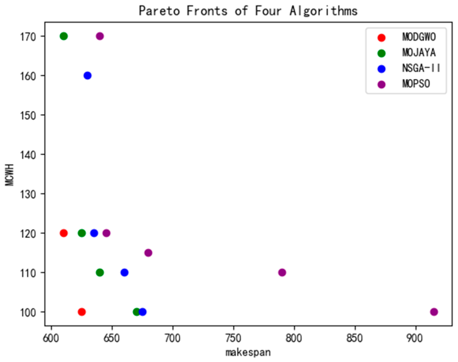
| Algorithms | Number of Solutions | Pareto Solutions |
|---|---|---|
| MODGWO | 2 | [610, 120], [625, 100] |
| MOJAYA | 4 | [610, 170], [625, 120], [640, 110], [670, 100] |
| NSGA-II | 4 | [635, 120], [630, 160], [660, 110], [675, 100] |
| MOPSO | 5 | [645, 120], [640, 170], [680, 115], [790, 110], [915, 100] |
Disclaimer/Publisher’s Note: The statements, opinions and data contained in all publications are solely those of the individual author(s) and contributor(s) and not of MDPI and/or the editor(s). MDPI and/or the editor(s) disclaim responsibility for any injury to people or property resulting from any ideas, methods, instructions or products referred to in the content. |
© 2025 by the authors. Licensee MDPI, Basel, Switzerland. This article is an open access article distributed under the terms and conditions of the Creative Commons Attribution (CC BY) license (https://creativecommons.org/licenses/by/4.0/).
Share and Cite
Wei, Z.; Yu, Z.; Niu, R.; Zhao, Q.; Li, Z. Research on Flexible Job Shop Scheduling Method for Agricultural Equipment Considering Multi-Resource Constraints. Agriculture 2025, 15, 442. https://doi.org/10.3390/agriculture15040442
Wei Z, Yu Z, Niu R, Zhao Q, Li Z. Research on Flexible Job Shop Scheduling Method for Agricultural Equipment Considering Multi-Resource Constraints. Agriculture. 2025; 15(4):442. https://doi.org/10.3390/agriculture15040442
Chicago/Turabian StyleWei, Zhangliang, Zipeng Yu, Renzhong Niu, Qilong Zhao, and Zhigang Li. 2025. "Research on Flexible Job Shop Scheduling Method for Agricultural Equipment Considering Multi-Resource Constraints" Agriculture 15, no. 4: 442. https://doi.org/10.3390/agriculture15040442
APA StyleWei, Z., Yu, Z., Niu, R., Zhao, Q., & Li, Z. (2025). Research on Flexible Job Shop Scheduling Method for Agricultural Equipment Considering Multi-Resource Constraints. Agriculture, 15(4), 442. https://doi.org/10.3390/agriculture15040442