Field Ridge Segmentation and Navigation Line Coordinate Extraction of Paddy Field Images Based on Machine Vision Fused with GNSS

Abstract

Farmland boundaries distinguish agricultural areas from non-agricultural areas, providing limits for field operations and navigation paths of agricultural machinery. However, in hilly regions, the irregularity of paddy field boundaries complicates the extraction of boundary information, hindering the widespread use of GNSS-based navigation systems in agricultural machinery. This paper focuses on the paddy field border prior to rice planting and utilizes machine vision and GNSS fusion technology to extract navigation line coordinates. First, the BiSeNet semantic segmentation network was employed to extract paddy field ridges. Second, the camera’s 3D attitude was obtained in real time using an Attitude and Heading Reference System (AHRS). A method and device based on the hydraulic profiling system were proposed to measure the camera’s height relative to the paddy field, providing a dynamic external reference. An improved inverse perspective transformation was applied to generate a bird’s-eye view of the paddy field ridges. Finally, a homogeneous coordinate transformation method was used to extract the navigation line coordinates, with the model and algorithms deployed on the Jetson AGX Xavier platform Field tests demonstrated a real-time segmentation speed of 26.31 fps, pixel segmentation accuracy of 92.43%, and an average intersection ratio of 90.62%. The average distance error of the extracted navigation line was 0.071 m, with a standard deviation of 0.039 m. The coordinate extraction took approximately 100 ms, meeting the accuracy and real-time requirements for navigation line extraction at the rice transplanter’s speed of 0.7 m s⁻¹, providing path information for subsequent autonomous navigation.

1. Introduction

Intelligent agricultural machinery, as the core component of modern agriculture, has shown revolutionary potential in alleviating labor shortages while enhancing operational precision and efficiency. It has become an essential technology for ensuring global food security and promoting sustainable agricultural development [1,2,3,4]. In recent years, GNSS (Global Navigation Satellite System)-based agricultural machinery navigation systems have successfully enabled autonomous operations in large-scale farmlands. These systems have been validated in typical agricultural applications, such as plowing, planting, and harvesting, in the plains of developed nations, where they have demonstrated significant technological advantages, with operational quality far surpassing traditional manual methods [5,6]. Agricultural machinery navigation technology, as a key and ubiquitous technology for intelligent agricultural machinery, directly impacts the modernization process of agricultural production [7].

Although GNSS navigation systems perform excellently in flat and regular farmlands, their application in hilly paddy fields faces significant technical challenges. The fundamental issue lies in the dependence of traditional operational modes on pre-established field boundary mapping conditions [8,9], which contradicts the complex terrain typical of hilly regions. Geographic fragmentation leads to small, high-curvature, and irregular spatial distributions of fields [10]. This exposes two key technical flaws of the GNSS system: (1) The discrete point path generation mechanism is inadequate for complex boundary topologies, and (2) the manual data collection method suffers from efficiency bottlenecks and cumulative errors. The combined impact of these deficiencies significantly increases the overall operational costs in hilly paddy fields and forms a critical bottleneck in the technology deployment [11]. To address the limitations of relying on a single positioning technology in particular environments, there is a pressing need to develop a multi-source perception fusion approach. Machine vision technology, with its real-time environmental perception and multi-dimensional feature fusion capabilities, can effectively address the gaps in GNSS system boundary information sensing [12]. By constructing a machine vision-GNSS multi-sensor fusion framework, the system’s environmental perception and boundary information accuracy are significantly improved [13], providing a reliable technical foundation for achieving high-precision autonomous navigation in intelligent agricultural machinery [14].

In the field of autonomous navigation for rice transplanters, the achievement of stable locomotion relies heavily on the accurate extraction of the navigation baseline [15]. As the initial step in environmental perception, farmland area segmentation methods can be classified into two categories: traditional algorithms based on manual feature selection and intelligent algorithms based on machine learning [16]. Among these, the Otsu thresholding algorithm maximizes inter-class variance in the image histogram, effectively separating the foreground from the background in simple scenarios [17]. The row-based grayscale transition feature rule proposed by Wang et al. [18] identifies headland boundaries through grayscale gradient analysis; however, it tends to produce segmentation errors in scenarios with uniform grayscale distributions in the field [19]. To enhance feature recognition, researchers commonly adopt color space transformation strategies (such as RGB to HSV conversion) or the Excess Green Index (ExG) for feature enhancement. Li et al. [20] constructed a high-dimensional feature space by combining color and texture features, integrating support vector machines (SVM) and superpixel segmentation techniques, thereby enabling high-precision identification of complex headland regions. However, traditional image processing methods have two major limitations: (1) they depend on manually designed local feature descriptors (such as color, texture, and shape) [21]; (2) they are highly complex in parameter tuning and lack environmental adaptability, particularly in unstructured farmland environments, where terrain fluctuations, weed interference, meteorological changes, and lighting anomalies, such as specular reflection and hot spots, severely limit the algorithm’s generalization capability [22]. In contrast, Convolutional Neural Networks (CNNs), through an end-to-end learning process, can directly extract multi-level spatial features from raw data, significantly enhancing algorithm adaptability and generalization ability [23]. With the iterative development of deep learning technologies, the application of neural networks in agricultural perception continues to deepen. For instance, He et al. [24] achieved precise extraction of ridge structures through semantic segmentation models, while Liu et al. [25] introduced elevation difference information to develop a multi-source data fusion model, effectively enhancing the stability of headland boundary detection.

The results of farmland area segmentation provide essential spatial information for navigation line extraction. Currently, the extraction of navigation lines primarily relies on line detection and fitting methods: Keun et al. [26] proposed a line intersection detection method based on the Hough transform, which can generate crop row guidance lines; however, it has high computational complexity and faces challenges in detecting peaks in multi-line scenarios [27]. The region-growing sequence clustering and RANSAC (Random Sample Consensus) combined algorithm proposed by Fu et al. [28] can fit seedling row centerlines, but its parameter sensitivity and computational complexity limit its practical applicability [29]. The least squares method, known for its computational efficiency and fitting accuracy, has been widely applied in visual navigation line extraction. For example, Diao et al. [30] employed an improved vertical projection method to obtain crop row feature points, followed by least squares fitting to extract navigation lines in complex farmland environments. It is important to note that existing research primarily focuses on linear fitting for farmland boundary or centerline detection, with a notable lack of studies on the path generation mechanisms for curved lines [31]. This gap hinders the ability to meet the navigation challenges posed by irregular boundaries in hilly rice fields.

The conversion of the navigation line into the executable path for agricultural machinery is fundamentally reliant on the achievement of high-precision coordinate positioning and mapping. The predominant methodologies in this domain include: (1) stereo vision-based 3D reconstruction; (2) LiDAR point cloud modeling; and (3) inverse perspective mapping (IPM) correction. The binocular stereo-matching algorithm developed by Hong et al. [32] facilitates the recognition and distance measurement of field ridge boundaries; however, its computational complexity limits its real-time applicability [33]. Ji et al. [34] employed LiDAR to construct terrain elevation models; nevertheless, this approach is constrained by high equipment costs and the cumulative errors arising from point cloud registration [35]. Liu et al. [36] enhanced the sliding window algorithm to improve adaptability within agricultural contexts, yet the design of fixed viewpoint transformation parameters fails to account for the dynamic coupling between terrain variations and camera pose. The three-dimensional reconstruction method based on stereo cameras, as proposed by S. Zhang et al. [37], exhibits a strong dependency on initial calibration parameters. Collectively, these methods are characterized by an implicit reliance on the assumption of flat terrain, which gives rise to two significant systemic limitations in more complex environments, such as hilly paddy fields: (1) Dynamic Projection Distortion: The coordinate mapping model, based on fixed parameters, is unable to accommodate variations in camera pose induced by terrain undulations, leading to the accumulation of path tracking errors. (2) Coordinate System Mapping Deficiencies: Existing research primarily focuses on the extraction of navigation lines within the image coordinate system, thereby inhibiting the integration with global coordinate systems (e.g., GNSS), which is necessary for the generation of absolute path coordinates capable of directly guiding autonomous agricultural machinery.

In response to the aforementioned technical challenges, the present study makes several significant contributions:

(1)

Embedded Real-time Semantic Segmentation System: A bilateral semantic segmentation network model (BiSeNet) is utilized to detect paddy field ridges. The system is optimized and deployed on the Jetson AGX Xavier platform, employing the TensorRT inference engine to facilitate the real-time detection of paddy field ridges.

(2)

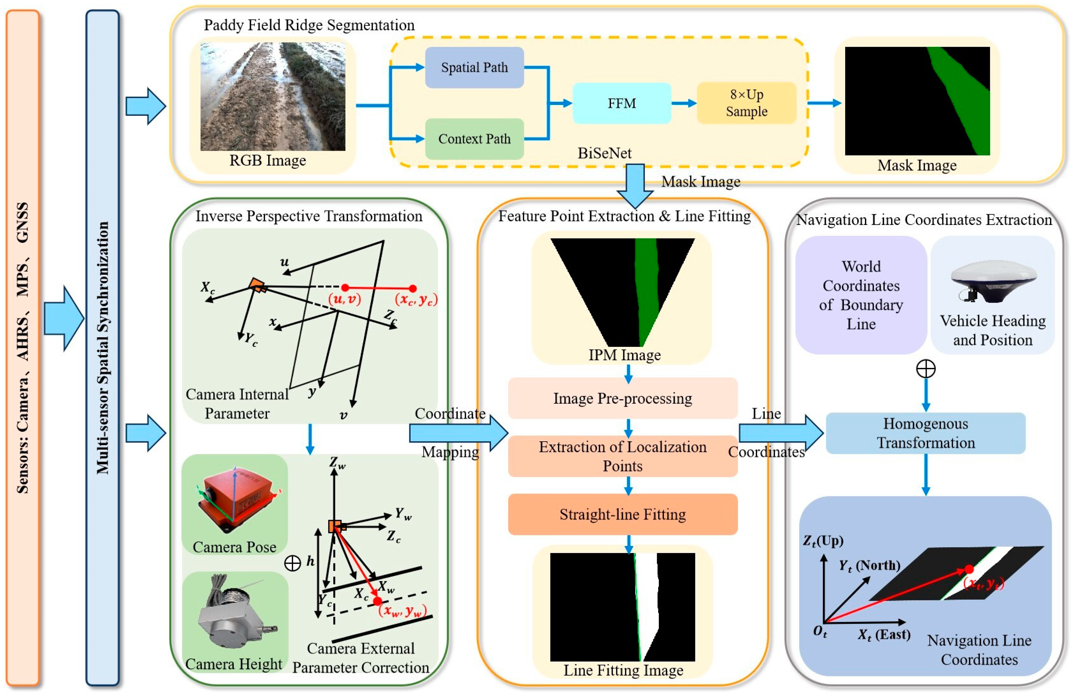
Multi-sensor Dynamic Perception Architecture: By integrating machine vision, GNSS, and AHRS (Attitude and Heading Reference System), a dynamic measurement model for the camera’s height above the ground is developed. An advanced, comprehensive inverse perspective mapping (IPM) algorithm is formulated to enable real-time transformation from image coordinates to navigation coordinates, irrespective of the camera’s pose.

(3)

Comprehensive Terrain Validation and Systematic Evaluation: A visual navigation testing platform for the rice transplanter is established, and field experiments are performed without prior boundary information. The results of these experiments validate the system’s accuracy, real-time performance, and stability in autonomously acquiring navigation and positioning data for paddy field ridges.

2. Materials and Methods

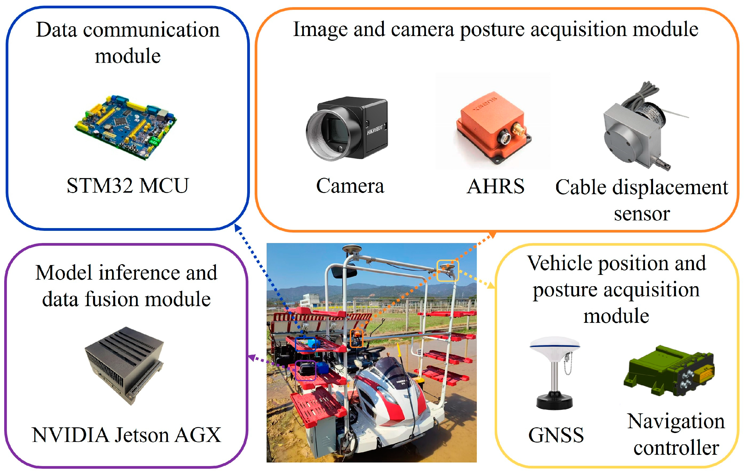
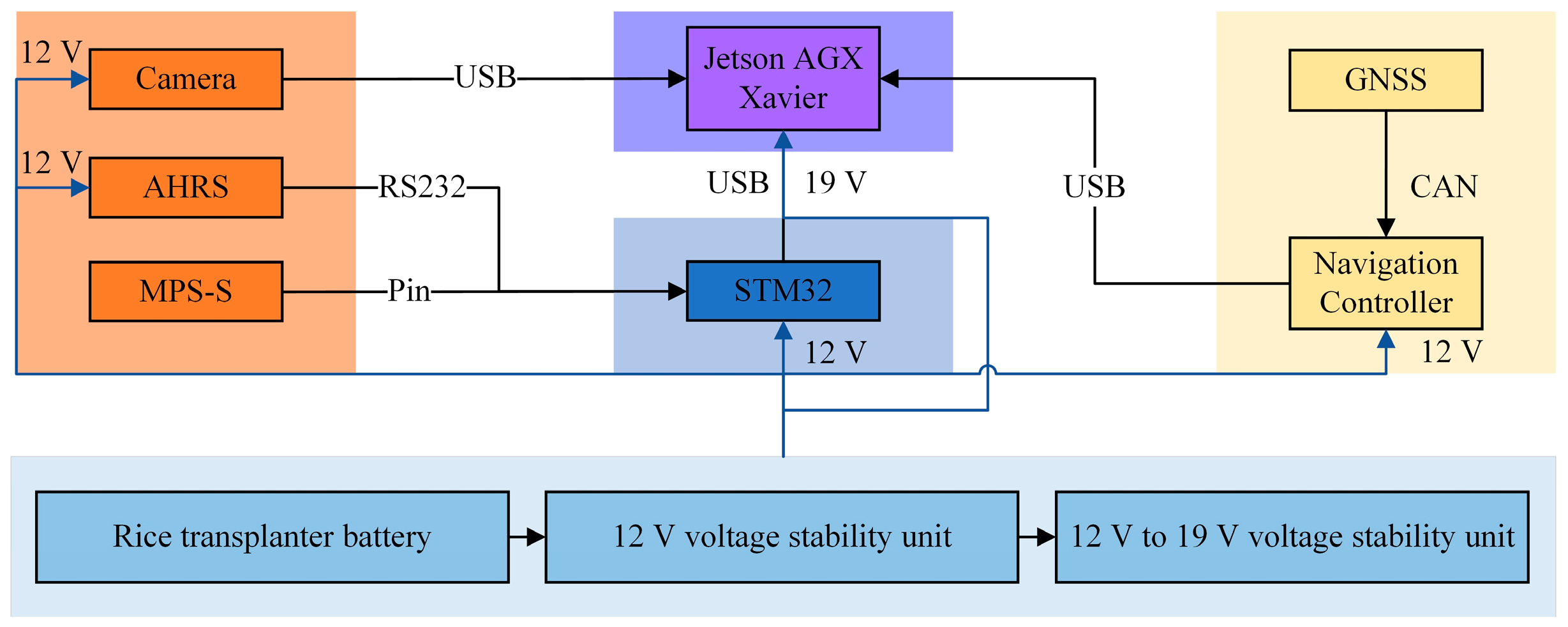
2.1. Platform Configuration

The model’s training and testing procedures were conducted on a workstation running the Ubuntu 18.04 operating system. The key specifications of the workstation were as follows: an NVIDIA RTX 5000 (with 16 GB of video memory) GPU and a CPU with the Intel Xeon 6142 processor. The model was developed using the Python 3.6 programming language within the PyTorch 1.8.0 deep learning framework. In addition, the semantic segmentation algorithm was executed on the GPU equipped with the CUDA 10.2 parallel programming platform and the cuDNN 7.6.5 acceleration package.

The schematic diagram of the data acquisition platform is shown in Figure 1. This platform is integrated into the Yanmar YR70D rice transplanter and comprises four primary modules: image and camera attitude acquisition, vehicle position and attitude acquisition, data communication, and model inference and data fusion. The system architecture is shown in Figure 2. All modules are interconnected through industrial-grade wired communication interfaces, including USB 3.0, RS-232, CAN bus, and pin connectors. The GNSS positioning system employs network RTK (Real-Time Kinematic) differential positioning technology, which receives correction data from a reference station via 4G LTE networks, thereby facilitating centimeter-level precision. In terms of the power supply design, the system is powered by the transplanter’s 12 V battery, which is subsequently converted to a stable 19 V operating voltage via a 12 V to 19 V DC-DC boost converter.

The image and camera attitude acquisition module incorporated a camera (MV-CA016-10UC, Hikvision, Hangzhou, China) positioned at the front end of the rice transplanter, enabling efficient one-time image acquisition. The AHRS (Mti-300, Xsens, Enschede, The Netherlands) provided camera poses, which could be represented by Euler angles, normalized quaternions, or rotation matrices. In addition, a pull cord displacement sensor (MPS-S-1000-V2, MILONT, Shenzhen, China) indirectly measured the camera height from the paddy field through calibration, with output values as the voltage.

The vehicle position and attitude acquisition module featured a GNSS receiver and navigation controller. A GNSS base station (CHCNAV I60, CHC Navigation, Shanghai, China) transmitted position deviation data via radio, while a GNSS mobile station with dual positioning antennas (UM982, Unicore Communications, Beijing, China) provided RTK position and heading information.

The data communication module used an STM32 microcontroller to package and transmit sensor data frames to the embedded development platform via a customized communication protocol.

The model inference and data fusion module comprised an embedded development platform (Jetson AGX Xavier, Nvidia, Santa Clara, CA, USA) responsible for deploying the model in the real environment. This platform also facilitated communication with all sensors. Specific models and parameters of the sensors used in the system are detailed in

Table 1. Sensor-specific models and parameters. Parameters are sourced from the official user manuals and product documentation.

Sensors	Models	Parameters
Camera	MV-CA016-10UC	Sensor model: IMX273
		Sensor type: CMOS
		Resolution: 1440 × 1080
		Maximum frame rate: 249.1 fps
		Connector: USB3.0
AHRS	MTi-300 (Xsens)	Roll (RMS): 0.2°
		Pitch (RMS): 0.2°
		Yaw (RMS): 1.0°
Cable displacement sensor	MPS-S-1000-V2	Sensor range (mm): 100–2500 mm
		Signal output (V): 0–10 V
GNSS	UM982	Channels: 1408
		Satellite: BDS/GPS/GLONASS/Galileo/QZSS
		Orientation Accuracy: 0.1°/1 m Baseline
		RTK(RMS): 0.8 cm ± 1 ppm (horizontal), 1.5 cm ± 1 ppm (vertical)
		Output frequency: 20 Hz

.

2.2. Image Acquisition and Dataset Construction

(1)

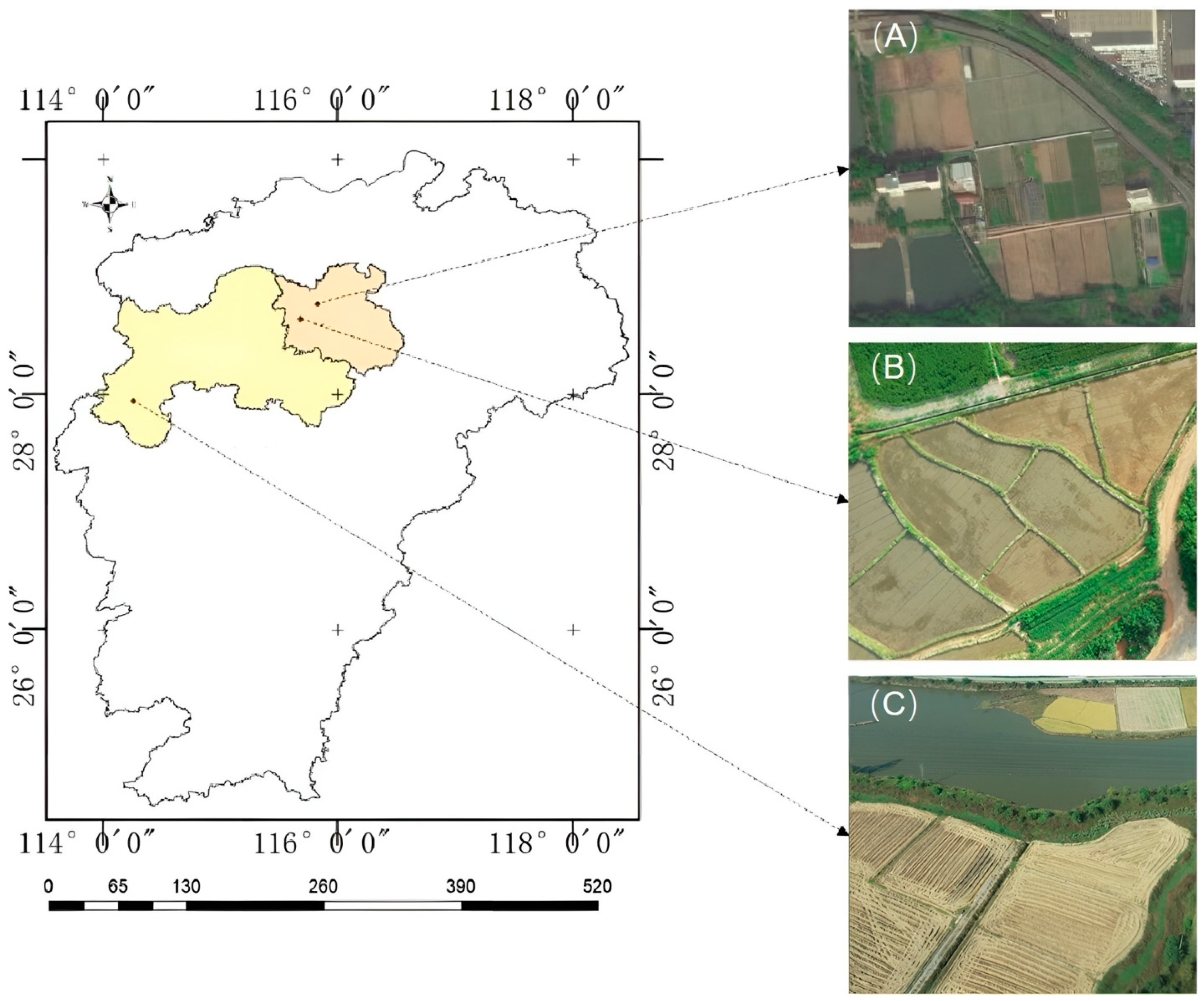
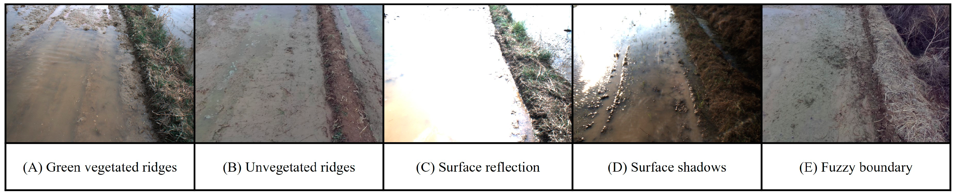
Image Acquisition

A Yanmar rice transplanter was used as the base platform to collect RGB images from the rice field. An industrial camera (MV-CA016-10UC, Hikvision, Hangzhou, China) was mounted on the right side of the crossbar, 1.5 m above the rice transplanter head. The front-view distance of the industrial camera is about 5 m, and the elevation angle is 35°. The camera takes images in JPG format, with a resolution of 1440 × 1080 pixels. The rice transplanter traveled along the edge of the field at a constant speed in automatic operating gear, the video stream was acquired in real time using the SDK provided by the Hikvon industrial camera, and the paddy field ridge images were intercepted every 10 frames of the video stream. The acquisition time of the paddy field ridge images was divided into four stages (18 January 2020; 5 March 2020; 18 April 2021; and 5 June 2021); the acquisition time period was from 7:00 a.m. to 11:00 a.m. and 2:00 p.m. to 5:00 p.m., which included three time periods of morning and noon; and the weather included cloudy and sunny days. The image acquisition sites were the North Experimental Field of Jiangxi Agricultural University (latitude 28°77′ N, longitude 115°83′ E); Ganzhu Farm in Yuanzhou District, Yichun City (latitude 114°26′ N, longitude 27°94′ E); and Kelicun Farm in Xinjian County, Nanchang City (latitude 115°68′ N, longitude 28°64′ E), as shown in Figure 3. The fields in the North Experimental Field are standardized fields, which are rectangular in shape and arranged in an orderly manner. Most of the fields in Ganzhu Farm are irregular and have different sizes and height differences, while those in Kelicun Farm are mainly plains in terms of terrain distribution, and the fields are flat but with mostly curved ridges.

Due to the complex environment of the paddy fields, data acquisition in the plowed fields was carried out in the early, middle, and late rice cultivation periods. The paddy field ridge images acquired in the early and middle rice cultivation periods were mainly of five types, as shown in Figure 4: scenes of green vegetation cover, no vegetation cover, water surface reflections, water surface shadows, and fuzzy boundary. The green vegetation cover images were collected in early June, with a large amount of green vegetation on the surface of the fields, typical of a paddy field after plowing and before rice transplanting. Images of fields without a vegetation cover were collected in early January (i.e., in the winter), with withered vegetation covering the surface of the fields and a small amount of water frozen on the field surface, along with some rice stubble stalks, which is typical of a fallow paddy field after harvesting in the winter. Water surface reflections were associated with the outdoor light intensity and caused a loss in imaging performance due to localized whitening of the paddy field content’s reflective region; this phenomenon mostly occurred in the summer at around midday. Shadow blocking due to oblique illumination from the sun, causing shadows on the fields, was mostly distributed in the morning and afternoon hours. Boundary blurring was caused by the brightness and color texture of dense weeds similar to that of paddy field ridges. After paddy field ridge images of the three rice-growing areas were obtained, we removed abnormal images and finally obtained a total of 1365 images.

(2)

Dataset construction

Paddy field ridge images were randomly selected to create a dataset, and the size of each image was 1440 × 1080 pixels. The dataset was labeled using the Labelme program, which uses polygon labels to train the BiSeNet image segmentation model, as depicted in Figure 5. The images were divided into a training set and a test set, with 956 images allocated for training and 409 images reserved for testing purposes.

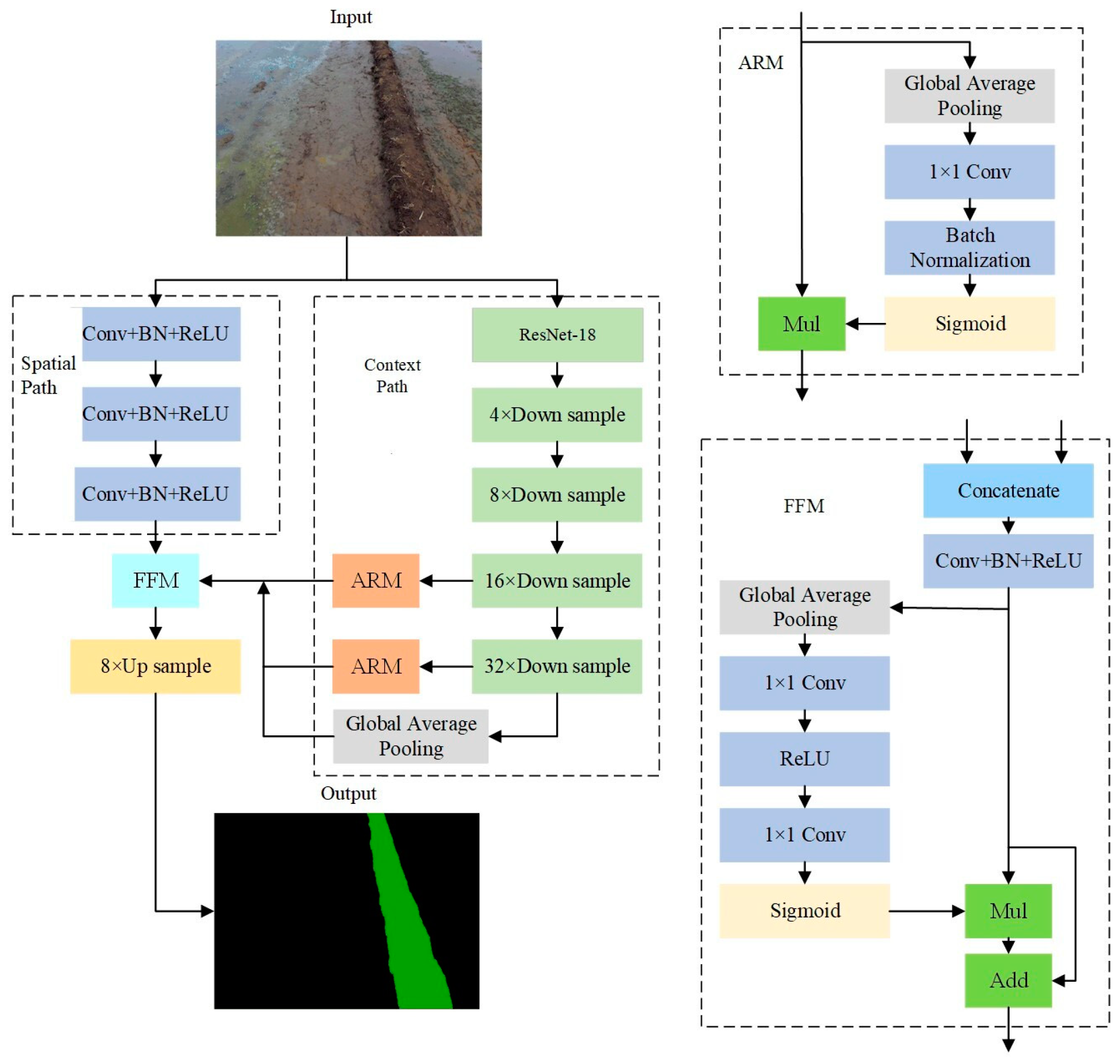
2.3. BiSeNet Network Model

To address the dual challenges of real-time processing demands and segmentation accuracy in agricultural applications, this study employed the Bilateral Segmentation Network (BiSeNet) [38]. This network achieves an effective balance between accuracy and efficiency by employing a spatial-context dual-path heterogeneous architecture. The spatial path preserves high-resolution spatial information, whereas the context path, through the implementation of lightweight context modeling, enhances both accuracy and efficiency.

Spatial Path (SP): This component is designed to maintain the spatial resolution of the input image and to encode high-resolution spatial features. The architecture of the network comprises three stages, each containing 3 × 3 convolutional kernels with a stride of 2, followed by batch normalization (BN) and a ReLU activation function. Following three down-sampling operations with a stride of 2, the spatial resolution of the feature maps is reduced to one-eighth of the original input. These high-resolution feature maps, encoded through a dense spatial feature encoding mechanism, considerably improve the representation of edge details within the paddy field ridge regions.

Context Path (CP): A lightweight ResNet-18 [39] architecture serves as the backbone for the context branch, effectively capturing high-level semantic context information through hierarchical down-sampling, which exponentially expands the receptive field. Stage 3 and Stage 4 output feature maps with 16× and 32× down-sampling, respectively, and further extract global semantic prior information via global average pooling (GAP).

Attention Refinement Module (ARM): To enhance the discriminability of features in the context branch, an ARM module is introduced. This module first generates a channel attention vector through global average pooling, subsequently compressing the channel dimension using a 1 × 1 convolutional layer. The resulting vector undergoes batch normalization and is processed through a Sigmoid activation function to generate channel attention weights. These weights are then applied to the feature maps of Stage 3 and Stage 4 through a channel-wise multiplication operation, facilitating collaborative optimization that suppresses noisy channels and accentuates target-related features.

Feature Fusion Module (FFM): The spatial and context branches extract low-level geometric details and high-level semantic context features, respectively. These features exhibit significant differences in terms of abstraction levels and information density. A direct addition of these features would result in the loss of detailed information due to semantic ambiguity. Consequently, the FFM module employs a channel-space dual-attention mechanism to adaptively combine features from both branches. The high-resolution features from the spatial path enhance the accuracy of boundary localization, while the broader receptive field features from the context path provide semantic consistency constraints. The fused features effectively preserve both pixel-level detail fidelity and object-level semantic integrity. The structure of the BiSeNet network is depicted in Figure 6.

2.4. Navigation Line Fitting for Paddy Field Ridges

The semantic segmentation network developed in Section 2.3 conducted pixel-level segmentation on paddy field ridge images (corresponding to Module: Paddy Field Ridge Segmentation in Figure 7), producing a mask image as the primary input data. To mitigate coordinate mapping discrepancies induced by terrain variations, the enhanced full-factor inverse perspective mapping (IPM) algorithm, introduced in Section 2.5 (corresponding to Module: Inverse Perspective Transformation in Figure 7), was implemented. This algorithm dynamically compensated for camera tilt and ground curvature, thereby establishing a precise geometric projection model that facilitated the transformation of coordinates from the pixel coordinate system to the world coordinate system.

Subsequently, the mask image and transformation matrix were processed within the Feature Point Extraction & Line Fitting module (corresponding to Module: Feature Point Extraction & Line Fitting in Figure 7). Utilizing the internal boundary localization and line fitting methodology delineated in Section 2.6, morphological operations and contour optimization algorithms were applied to the IPM-transformed image to extract critical feature points along the inner ridge boundary. The least squares method was then employed to determine the parametric equation of the boundary line, ultimately yielding the world coordinate parameters of the ridge geometry.

During the navigation line coordinate transformation stage (corresponding to Module: Navigation Line Coordinates Extraction in Figure 7), the homogeneous coordinate transformation method outlined in Section 2.7 was utilized to integrate the extracted boundary coordinates with GNSS positioning data and dual-antenna heading information, thereby mapping these elements to the global navigation coordinate system of the agricultural machine.

More specifically, the inverse perspective mapping established the geometric projection relationship between the pixel plane and the world plane, while the homogeneous coordinate transformation applied an affine matrix to achieve scale normalization and coordinate adaptation within the agricultural machine’s navigation system. The final output consisted of an absolute coordinate sequence optimized for autonomous agricultural navigation.

The directional arrows in Figure 7 explicitly depict the sequential data flow from the raw image input to the navigation coordinate output, illustrating the modular interaction within a cascaded framework to ensure functional integration and coherence.

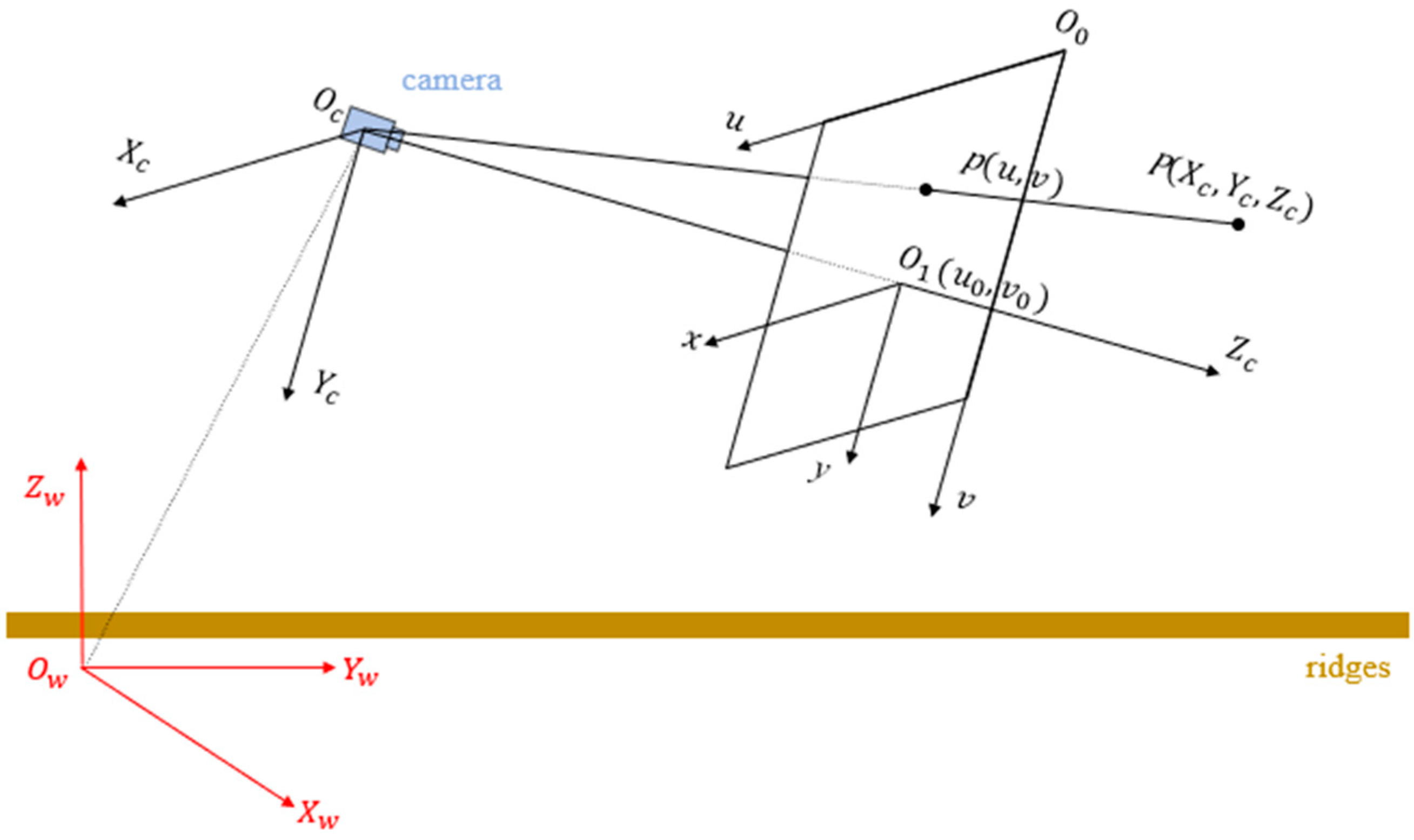
2.5. Acquisition of an Aerial View of Paddy Field Ridges Based on Inverse Perspective Transformation

After applying BiSeNet semantic segmentation, the mask images of paddy field ridges exhibited a perspective effect, with objects appearing larger when they were nearer and smaller when they were farther away, due to the camera’s imaging principle. To accurately represent the actual positional relationship between the rice transplanter and the field ridges and to calculate the distance between them, it was necessary to eliminate the perspective effect from the paddy field ridge images captured by the camera by using an inverse perspective transformation. This process allowed obtaining a bird’s-eye view of the paddy field ridges.

(1)

Inverse perspective transformation

The purpose of inverse perspective transformation is to restore the camera’s image pixel coordinates back to the physical world coordinate system, thereby obtaining a bird’s-eye view of the image. The fundamental principle of camera imaging involves mapping physical coordinate points from the physical world coordinate system to the pixel coordinate system, essentially reversing the process of camera imaging. This inverse perspective transformation process is illustrated in Figure 8.

The inverse perspective transformation of the camera involves the conversion of four coordinate systems: the world coordinate system to the camera coordinate system, the camera coordinate system to the image coordinate system, and the image coordinate system to the pixel coordinate system.

The conversion from the world coordinate system $O_w$-$X_w{Y}_w{Z}_w$ to the camera coordinate system $O_c$-$X_c{Y}_c{Z}_c$ can be represented as follows:

$$\left[\begin{array}{c}\begin{array}{c}{x}_c\\ y_c\\ z_c\end{array}\\ 1\end{array}\right]=\left[\begin{array}{ccc}{R}_{3\times 3}& ⋮& T_{3\times 1}\\ \cdots & ⋮& \cdots \\ 0& ⋮& 1\end{array}\right]\cdot \left[\begin{array}{c}\begin{array}{c}{x}_w\\ y_w\\ z_w\end{array}\\ 1\end{array}\right]$$

(1)

where $(x_c,y_c,z_c)$ are the coordinates under the camera coordinate system, $R$ denotes the rotation matrix, $T$ denotes the displacement matrix, and $(x_w,y_w,z_w)$ are the coordinates under the world coordinate system.

The conversion from the camera coordinate system $O_c$-$X_c{Y}_c{Z}_c$ to the image coordinate system $O_1$-$xy$ can be represented as follows:

$$z_c\left[\begin{array}{c}x\\ y\\ 1\end{array}\right]=\left[\begin{array}{c} f \\ 0\\ 0\end{array}\begin{array}{c} 0\\ f\\ 0\end{array}\begin{array}{c} 0\\ 0\\ 1\end{array}\begin{array}{c} 0\\ 0 \\ 0\end{array}\right]\cdot \left[\begin{array}{c}\begin{array}{c}{x}_c\\ y_c\\ z_c\end{array}\\ 1\end{array}\right]$$

(2)

where $(x,y)$ are the coordinates under the image coordinate system and $f$ is the camera’s focal length.

The conversion from the image coordinate system $O_1$-$xy$ to the pixel coordinate system $O_0$-$uv$ can be represented as follows:

$$\left[\begin{array}{c}u\\ v\\ 1\end{array}\right]=\left[\begin{array}{ccc}{\displaystyle \frac{1}{dx}}& 0& c_x\\ 0& {\displaystyle \frac{1}{dy}}& c_y\\ 0& 0& 1\end{array}\right]\cdot \left[\begin{array}{c}x\\ y\\ 1\end{array}\right]$$

(3)

where $(u,v)$ are the coordinates under the pixel coordinate system, $dx$ is the physical dimensions of the pixel in the $X$-axis direction, $dy$ is the physical dimensions of the pixel in the $Y$-axis direction, and $(c_x,c_y)$ is the camera’s optical center.

According to Equations (1)–(3), the expression for converting coordinates $(x_w,y_w,z_w)$ in the world coordinate system to coordinates $\left(u,v\right)$ in the pixel coordinate system is given by Equation (4), which represents the camera’s inverse perspective transformation:

$$Z_c\left[\begin{array}{c}u\\ v\\ 1\end{array}\right]=\left[\begin{array}{ccc}{\displaystyle \frac{1}{dx}}& 0& u_0\\ 0& {\displaystyle \frac{1}{dy}}& v_0\\ 0& 0& 1\end{array}\right]\cdot \left[\begin{array}{cccc}\begin{array}{c}f\\ 0\\ 0\end{array}& \begin{array}{c}0\\ f\\ 0\end{array}& \begin{array}{c}0\\ 0\\ 1\end{array}& \begin{array}{c}0\\ 0\\ 0\end{array}\end{array}\right]\cdot \left[\begin{array}{cc}R& T\\ 0& 1\end{array}\right]\cdot \left[\begin{array}{c}{x}_w\\ y_w\\ z_w\\ 1\end{array}\right]$$

(4)

Aly et al. [40] introduced a robust and real-time inverse perspective transformation method for lane-marking detection on urban streets. This method generates a 2D top-view that accurately reflects the relationship with the actual position of the camera. The proposed inverse perspective transformation formula is presented in Equation (5):

$$\left[\begin{array}{c}{x}_w\\ y_w\\ -h\\ 1\end{array}\right]=h\left[\begin{array}{cccc}-c_2{\displaystyle \frac{1}{f_u}}& s_1{s}_2{\displaystyle \frac{1}{f_v}}& c_u{c}_2{\displaystyle \frac{1}{f_u}}-c_v{s}_1{s}_2{\displaystyle \frac{1}{f_v}}-c_1{s}_2& 0\\ s_2{\displaystyle \frac{1}{f_u}}& s_1{c}_1{\displaystyle \frac{1}{f_v}}& -c_u{c}_2{\displaystyle \frac{1}{f_u}}-c_v{s}_1{c}_2{\displaystyle \frac{1}{f_v}}-c_1{s}_2& 0\\ 0& c_1{\displaystyle \frac{1}{f_v}}& -c_v{c}_1{\displaystyle \frac{1}{f_v}}+s_1& 0\\ 0& -c_1{\displaystyle \frac{1}{h{f}_v}}& c_v{c}_1{\displaystyle \frac{1}{h{f}_v}}& 0\end{array}\right]\cdot \left[\begin{array}{c}u\\ v\\ 1\\ 1\end{array}\right]$$

(5)

where $c_1=\mathit{cos}\alpha$, $c_2=\mathit{cos}\beta$, $s_1=\mathit{sin}\alpha$, $s_2=\mathit{sin}\beta$, $\alpha$ is the pitch angle of the camera, $\beta$ is the yaw angle of the camera, f_u and f_v denote the focal lengths of the camera, and c_u and c_v denote the optical center points of the camera. These parameters are determined through the calibration of the camera [41]. This inverse perspective transformation formula establishes the origin of the world coordinates at the camera origin and the Z_c-axis of the camera coordinate system at the camera’s optical axis but only considers the case where the camera exists in pitch and yaw angles.

(2)

Camera roll attitude correction

Unlike the scenario on a relatively flat highway, where only the pitch and yaw angles of the camera are considered, in the paddy field environment, the roll angle of the camera also becomes significant. This study used and improved upon the inverse perspective transformation matrix proposed in Equation (5) for application in paddy field environments where rice transplanters operate. To incorporate the camera’s roll attitude, the method involved measuring the camera’s 3D attitude angle using an AHRS attitude sensor. The camera’s traverse roll attitude was then added, and the correction method involved rotating the camera’s imaging picture around its optical center. The rotation transformation matrix M for the image around the camera’s optical center can be obtained using the cv2.getRotationMatrix2D() function in OpenCV, and then applied through affine transformation using the cv2.warpAffine() function. As shown in Equation (6), the affine-transformed image is used to replace the captured camera image in Equation (5).

$$\left[\begin{array}{c}u\\ v\end{array}\right]=M\cdot \left[\begin{array}{c}{u}_0\\ v_0\\ 1\end{array}\right]=\left[\begin{array}{ccc}\begin{array}{c}\mathit{cos}\gamma \\ \mathit{sin}\gamma \end{array}& \begin{array}{c}-\mathit{sin}\gamma \\ \mathit{cos}\gamma \end{array}& \begin{array}{c}{c}_u\left(1-\mathit{cos}\gamma \right)+c_v\mathit{sin}\gamma \\ c_v\left(1-\mathit{cos}\gamma \right)-c_u\mathit{sin}\gamma \end{array}\end{array}\right]·\left[\begin{array}{c}{u}_0\\ v_0\\ 1\end{array}\right]$$

(6)

where $\gamma$ represents the inverse of the camera’s roll angle, $c_u$ and $c_v$ represent the camera’s optical center points, $M$ represents the transformation matrix, $(u_0,v_0)$ are the initial pixel coordinates of the camera image capture, and $\left(u,v\right)$ represent the pixel coordinates after affine transformation.

(3)

Camera height parameter correction

In waterlogged paddy fields characterized by uneven terrain and variable depths of soft mud, the significant jolting of agricultural machinery induced continuous fluctuations in the camera’s height relative to the field surface. Consequently, the projection parameters within the inverse perspective transformation matrix (Equation (5)) became misaligned, resulting in coordinate mapping errors. To improve the real-time correction of these parameters, this study introduced an onboard camera height-sensing system based on a hydraulic profiling mechanism, as shown in Figure 9A. By incorporating a closed-loop control framework that accounted for terrain fluctuations through mechanical adaptation, parameter calibration, and error mitigation, the proposed system enhanced mapping accuracy.

The Yanmar rice transplanter platform was equipped with an automatic transplanting profiling control system. Within this system, the floating plate (Component 6) functioned as a contact-based terrain sensing unit, mechanically linked to a hydraulic control valve assembly via a rigid linkage mechanism. Variations in the paddy field surface induced vertical displacement of the floating plate, leading to its physical deformation, which is subsequently transmitted through a lever mechanism. This process activated the proportional directional valve, thereby regulating hydraulic circuit pressure and driving the extension or retraction of the hydraulic cylinder’s piston rod (Component 2). The hydraulic cylinder, in turn, actuated a parallel four-bar linkage mechanism (Component 4), transforming the cylinder’s displacement into vertical movement of the transplanting platform (Component 5). Owing to its geometric constraints, this mechanism effectively eliminated lateral displacement, ensuring that the platform moves strictly along the vertical axis while maintaining the horizontal stability of the camera installation.

Given that the camera’s installation position remains rigidly fixed, a linear relationship between its displacement and variations in platform height was established through calibration experiments, as formulated in Equation (7).

$$\left\{\begin{array}{c}∆h=k\times l+b\\ h=h_0-∆h\end{array}\right.$$

(7)

where $∆h$ represents the variation in the height of the transplanting platform, $l$ represents the extension of the hydraulic cylinder, $k$ and $b$ are calibration coefficients, $h_0$ represents the initial installation height of the camera, and $h$ represents the camera’s height relative to the paddy field surface. This information was utilized to correct the height parameters in Equation (5) of the proposed perspective transformation matrix.

Therefore, this study adopted the method of measuring the extension of the hydraulic cylinder to obtain the camera’s height above ground level. The chosen sensor for measuring the extension of the hydraulic cylinder was the MPS-S-1000-V2 draw-wire displacement sensor, as shown in Figure 9B.

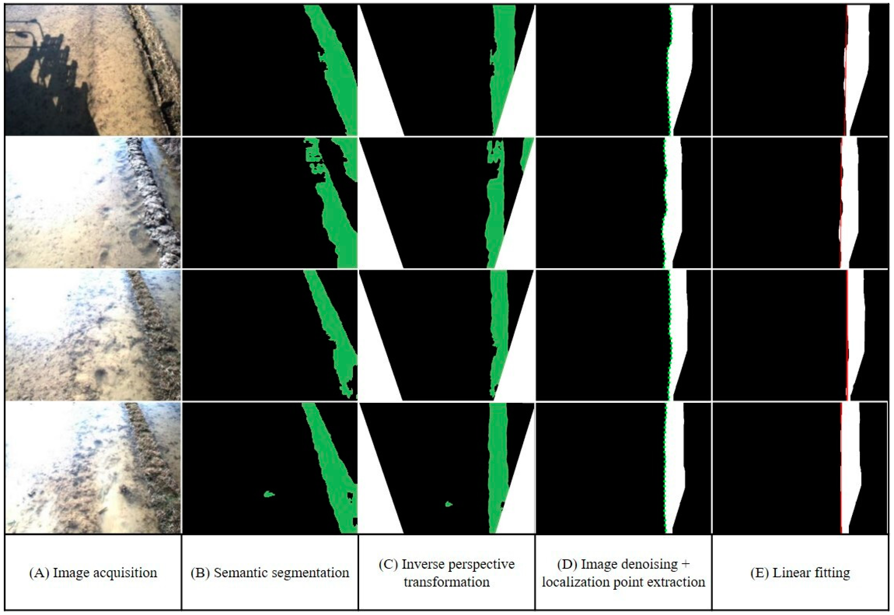
2.6. Straight-Line Fitting of Paddy Field Ridges Based on Distance Transformation

Inverse perspective transformation effectively generated an inverse perspective image of the segmented paddy field ridges, accurately reflecting their positional relationship in the real world. Building upon this, the inverse perspective image underwent denoising using digital image processing. Subsequently, positioning points along the paddy field ridge line were extracted and fitted. The resulting fitted ridge line served as the navigation data line for guiding the subsequent operation of the rice transplanter.

(1)

Image pre-processing

In the complex environment of paddy fields, noise interference may persist in the images of paddy field edge rows, even after semantic segmentation and inverse perspective transformation. This can lead to incorrect recognition of the exposed soil on the paddy field surface as edge rows or contaminants on the edge rows, resulting in segmentation omissions. To address these challenges, our study used several image processing techniques. First, we binarized the images post-inverse perspective transformation and eliminated connected regions with an area below a specified threshold. This process helped remove mis-segmented regions from the images. In addition, we used morphological closure operations, initially expanding and then eroding the images, to eliminate cavity noise in the binarized images of the paddy field ridges. This operation enhanced the boundary of the ridges, resulting in smoother ridge curves. These pre-processing steps are crucial for improving the accuracy and reliability of segmentation results in the challenging paddy field environment.

(2)

Extraction of localization points for paddy field ridges

After the denoising process, this study used distance transformation to extract the pixel coordinates of the paddy field ridges’ inner contour. Distance transformation calculates the distance from each non-zero pixel point (representing the foreground target, typically labeled as 1) to the nearest zero pixel point (background, labeled as 0) in the binary map. Therefore, in the binary map of paddy field ridges, distance transformation computed the shortest distance between each pixel point on the ridges and the background. This calculation provided position information about the inner boundary points of the ridges, allowing for their precise extraction and localization.

(3)

Straight-line fitting of paddy field ridges

When the camera is installed with a pitch angle of 30°, the camera’s field of view can cover approximately 4 m of the paddy field ridge length. Therefore, the paddy field ridge boundary in each frame of the image can be approximated as a straight line. As the camera continuously updates the images, the fitted straight line dynamically adjusts and gradually accumulates the overall irregularity of the paddy field ridge boundary. This method represents the paddy field ridge boundary as a curve composed of interconnected line segments. In this study, the inner boundary points of the paddy field ridge were extracted from a single frame image, followed by linear fitting. The coordinate mapping relationship was then used to obtain the boundary line’s world coordinates, laying the foundation for the subsequent generation of navigation lines.

Considering the relatively simple shape type of paddy field ridges, this study used the least squares method for straight-line fitting. This method offers advantages such as a low time complexity for fitting straight lines and a fast processing speed, and it meets the real-time requirements of agricultural machinery navigation. The resulting fitted straight line was plotted in the inverse perspective transformed images of the paddy field ridges, depicted with a red line in Figure 10. This line served as a reference for guiding the navigation of the rice transplanter along the edges of the paddy field ridges.

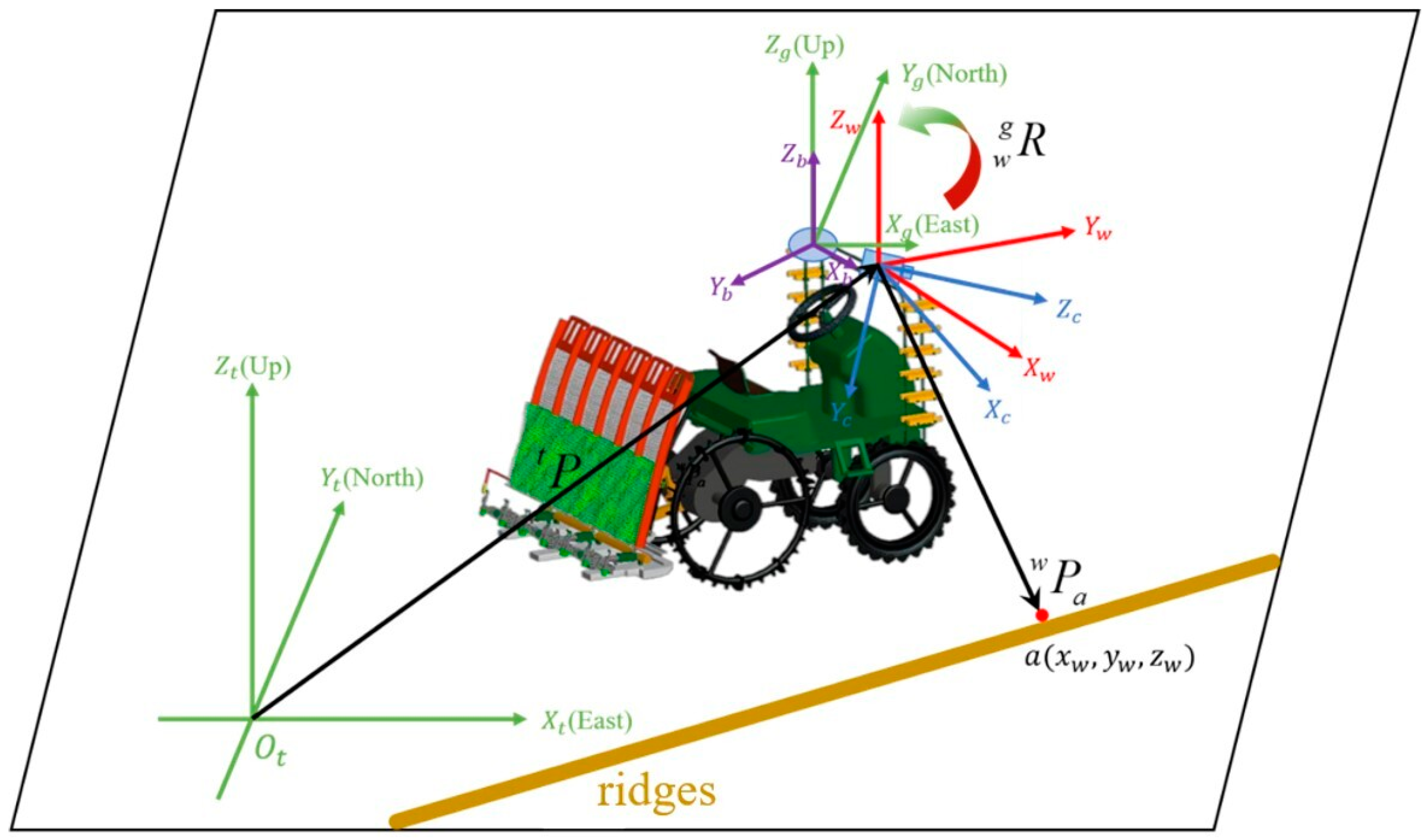
2.7. Coordinate Extraction of Navigation Lines of Paddy Field Ridges Based on Homogeneous Coordinate Transformation

By using semantic segmentation and inverse perspective transformation on paddy field ridges, as well as extracting and fitting them, this study enabled the acquisition of world coordinates for paddy field ridges. Building on this foundation, we proceeded to convert the position coordinates of the paddy field ridgeline from a local coordinate system to a global coordinate system using homogeneous coordinate transformation. This process involves four coordinate systems: the camera coordinate system$O_c$-$X_c{Y}_c{Z}_c$, the world coordinate system $O_w$-$X_w{Y}_w{Z}_w$, the vehicle body coordinate system$O_b$-$X_b{Y}_b{Z}_b$, and the navigation coordinate system${ O}_t$-$X_t{Y}_t{Z}_t$. The transformation relationship between these coordinate systems is illustrated in Figure 11. The transformation from the world coordinate system to the navigation coordinate system requires real-time position and attitude data. Moreover, the accuracy of the sidetrack position coordinate and positioning data may be compromised due to attitude changes caused by the uneven surface of the farmland. To address this, this study collected traverse and pitch data provided by the AHRS and heading data provided by the dual-antenna GNSS, aiming to compensate for the bias in the positioning information.

The process of converting the pixel coordinates of the paddy field ridges’ fitted straight line to the coordinates in the navigation coordinate system through the fusion of positional multi-sensor information and homogeneous coordinate transformation via inverse perspective transformation can be outlined as follows: The position coordinates of the camera in the $t$ system are obtained through homogeneous coordinate transformation. The camera is rigidly attached to the rice transplanter and moves along with it in the field, experiencing displacement and rotation relative to the $t$ system in the navigation coordinate system. This can be represented as the spatial vector ${}_{ }{}^b{p}_c$, which describes the displacement and rotation in the $t$ system. According to the $g$ and$b$ systems defined herein, the displacement vector is the coordinate of the antenna position in the $t$ system, denoted by${}_{ }{}^t{p}_{bO}$; since the $g$ system is parallel to the $t$ system, the rotation vector can be described as the orientation of the $b$system in the $g$system (or the $t$ system) ${}_b{}^{g}R$ (or ${}_b{}^{t}R$). According to this description and homogeneous coordinate transformation, the coordinates of the camera position in the $t$ system, which is solidly connected to the rice transplanter, are denoted by ${}_{ }{}^t{p}_{cO}$, which can be obtained with Equation (8):

$$\left[\begin{array}{c}{}_{ }{}^t{p}_{cO}\\ \cdots \\ 1\end{array}\right]=\left[\begin{array}{ccc}{}_b{}^{t}R& ⋮& {}_{ }{}^t{p}_{bO}\\ \cdots & ⋮& \cdots \\ 0 0 0& ⋮& 1\end{array}\right]\cdot \left[\begin{array}{c}{}_{ }{}^b{p}_c\\ \cdots \\ 1\end{array}\right]$$

(8)

where ${}_b{}^{t}R$ is a rotation transformation matrix constructed based on the Euler angle orientation description of the $b$system with respect to the $t$ system. Its physical meaning is the coordinate value of a vector whose three-axis coordinates on the $t$ system is 1 under the $b$coordinate system when the $t$ system is made to coincide with the $b$system by rotating a certain angle along the three coordinate axes sequentially.

In this paper, the orientation of the rice transplanter in the $b$ system is described based on the attitude angles $(\phi ,\theta ,\psi )$, the roll angle of the vehicle body around the $x$-axis of the $b$system, the pitch angle of the $y$-axis, and the heading angle of the $z$-axis. In addition, the attitude angle itself describes the orientation of the coordinate system resulting from the angle of rotation of the $b$ system in the $t$ system state along that particular sequential process of X-Y-Z, and the roll, pitch, and heading angles measured and output by the navigation controller are the attitude angles of the body. Therefore, the construction method of the rotation matrix,${}_b{}^{t}R$ is obtained using Equation (9), left-multiplying the rotation matrix of the corresponding axes sequentially in the order of rotation.

$$\begin{array}{l}{}_b{}^{t}R={}_{\psi }{}^{z}R\cdot {}_{\theta }{}^{y}R\cdot {}_{\phi }{}^{x}R\\ =\left[\begin{array}{ccc}cos\psi & -sin\psi & 0\\ sin\psi & cos\psi & 0\\ 0& 0& 1\end{array}\right]\cdot \left[\begin{array}{ccc}cos\theta & 0& sin\theta \\ 0& 1& 0\\ -sin\theta & 0& cos\theta \end{array}\right]\cdot \left[\begin{array}{ccc}1& 0& 0\\ 0& cos\phi & -sin\phi \\ 0& sin\phi & cos\phi \end{array}\right]\\ =\left[\begin{array}{ccc}cos\theta cos\psi & sin\phi sin\theta cos\psi -cos\phi sin\psi & cos\phi sin\theta cos\psi +sin\phi sin\psi \\ cos\theta sin\psi & sin\phi sin\theta sin\psi +cos\phi cos\psi & cos\phi sin\theta sin\psi -sin\phi cos\psi \\ -sin\theta & sin\phi cos\theta & cos\phi cos\theta \end{array}\right]\end{array}$$

(9)

Here, ${}_b{}^{t}R$ is a rotation transformation matrix constructed based on the Euler angle orientation description of the vehicle body coordinate system with respect to the navigation coordinate system, ${}_{\phi }{}^{x}R$, ${}_{\theta }{}^{y}R$, and ${}_{\psi }{}^{z}R$ are rotation matrices describing the vehicle body coordinate system orientation formed by rotating the vehicle body coordinate system by the angle of rotation along the corresponding coordinate axes in the state of the geographic coordinate system; $\phi$is the roll angle of the vehicle body about the $x$-axis of the vehicle body coordinate system; $\theta$is the pitch angle of the vehicle body about the $y$-axis of the vehicle body coordinate system; and $\psi$ is the heading angle of the vehicle body about the $z$-axis of the vehicle body coordinate system.

The world coordinates of the fitted straight line of the paddy field ridges were obtained based on the inverse perspective transformation fusion of positional multi-sensors in Section 2.5 and Section 2.6, and then, the coordinates of the navigation line of the paddy ridges were extracted using Equation (10) based on homogeneous coordinate transformation.

$$\left[\begin{array}{c}{}_{ }{}^t{p}_a\\ \cdots \\ 1\end{array}\right]=\left[\begin{array}{ccc}{}_w{}^{t}R& ⋮& {}_{ }{}^t{p}_{cO}\\ \cdots & ⋮& \cdots \\ 0 0 0& ⋮& 1\end{array}\right]\cdot \left[\begin{array}{c}{}_{ }{}^w{p}_a\\ \cdots \\ 1\end{array}\right]$$

(10)

Here, ${}_{ }{}^w{p}_a$is a space vector describing any vector point$\left(x_w,y_w,z_w\right)$of the field line, ${}_{ }{}^t{p}_a$ refers to the coordinates of the corresponding vector point of the field line in the navigational coordinate system, and the displacement vector ${}_{ }{}^t{p}_{cO}$ refers to the positional coordinates of the camera in the $t$ system, which is obtained using Equation (8). The rotation vector is described as the orientation ${}_w{}^{g}R$(or ${}_w{}^{t}R$) of the $w$ system in the $g$ system (or $t$ system).

3. Results and Analysis

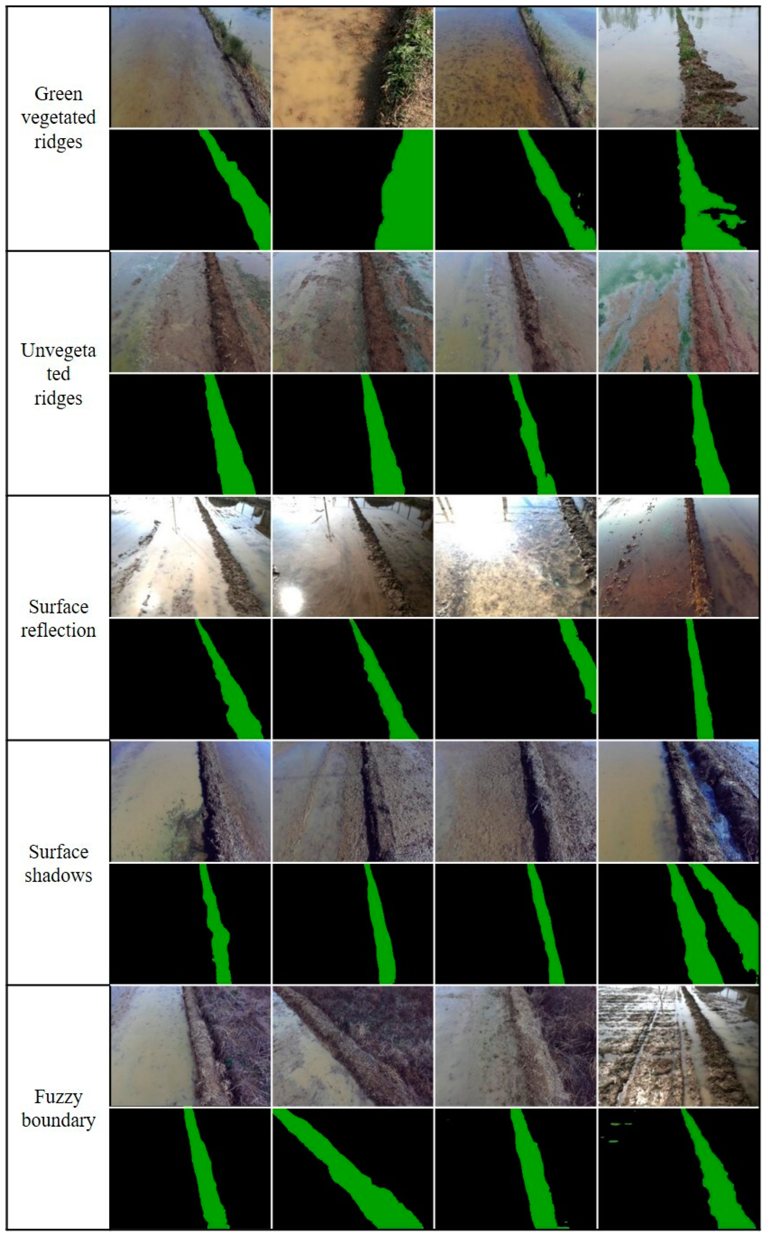
3.1. Recognition of Paddy Field Ridges

(1)

Model training

The proposed model was initialized with pre-trained ResNet18 weights from the Cityscapes dataset. Model optimization was performed using the stochastic gradient descent (SGD) algorithm, with specific parameters set as follows: initial learning rate of 0.0025, momentum factor of 0.9, weight decay coefficient of 0.0001, and dynamic adjustment of the learning rate using the Poly method. The batch size was set to 4, and the maximum number of iterations was set to 16 × 10⁴. The cross-entropy loss function was used during training, and the model was saved every 4000 iterations. The training process of the BiSeNet paddy field ridge segmentation model is illustrated in Figure 12, showing the change in iteration loss over training iterations. The loss curve gradually converged and stabilized around 14 × 10⁴ iterations, with the final model achieving a loss value of 0.124.

The pixel accuracy (Acc), mean intersection over union (mIoU), and segmentation speed (fps) were used to evaluate the final trained model and compare it with popular semantic segmentation models from recent years, such as PSPNet, UNet, and Deeplabv3+. The evaluation results are presented in

Table 2. Comparison results of model segmentation.

Model	Acc (%)	mIoU (%)	Segmentation Speed (fps)
PSPNet	89.39	82.89	6.67
UNet	89.86	84.24	6.81
Deeplabv3+	93.12	86.41	6.46
BiSeNet	92.61	90.88	18.87

. The model underwent testing for inference using 409 test images, and the average processing time per segmentation was calculated to determine the model’s segmentation speed. The results from the BiSeNet model’s segmentation indicated a pixel accuracy of 92.61%, an average intersection and merger ratio of 90.88%, and a segmentation speed of 18.87 fps, effectively balancing segmentation accuracy and inference speed.

Figure 13 shows a graph demonstrating the test segmentation results of the BiSeNet model for various types of paddy field ridges.

(2)

Model deployment

In this study, the BiSeNet paddy field ridge segmentation model was deployed and tested on Jetson AGX Xavier using TensorRT for model deployment, with three different data accuracies: FP32, FP16, and INT8. In addition, two different image input sizes were considered: 1024 × 1024 and 512 × 1024. The model performance was evaluated, and the test results are presented in

Table 3. BiSeNet model optimized for deployment testing using TensorRT.

Model	Performance Indicator	Image Resolution
		1024 × 1024	512 × 1024
PyTorch-FP32	fps	5.4933	5.6395
	MB	102.55	102.55
	mIoU	90.8403%	88.9504%
	Acc	92.5697%	90.1361%
TensorRT-FP32	fps	11.2456	20.3995
	MB	130.56	128.84
	mIoU	90.6256%	81.7504%
	Acc	92.4321%	86.1361%
TensorRT-FP16	fps	26.31269	38.6020
	MB	26.76	26.91
	mIoU	90.6245%	81.7621%
	Acc	92.4313%	86.1439%
TensorRT-INT8	fps	34.8101	42.6858
	MB	16.02	14.54
	mIoU	86.5943%	78.0418%
	Acc	88.4083%	82.3285%

.

Table 3 shows that the model segmentation speed reached 11.2456 fps, which is roughly twice as fast as the unoptimized model’s segmentation speed when the model was optimally deployed using TensorRT without changing the data accuracy at an image input resolution of 1024 × 1024. By reducing the data accuracy to FP16 and INT8, the model segmentation speed increased to 4.8 times and 6.3 times the original speed, respectively, after optimization. This resulted in speeds exceeding 25 fps, meeting real-time requirements and reducing the model size by 74% and 84%, respectively, compared to that of the original model. At FP32 and FP16 data accuracy levels, the model’s mean intersection over union (mIoU) and pixel accuracy (Acc) metrics remained largely unchanged compared to those of the unoptimized model. However, at INT8 data accuracy, compared to the optimized model, the mIoU decreased by 4.25 percentage points and the Acc decreased by 4.16 percentage points. This indicates that while INT8 data accuracy significantly reduces the model size and improves the segmentation speed, it also results in a notable loss of segmentation accuracy. Under FP16 data accuracy, TensorRT optimizes the model effectively, enhancing the segmentation speed without compromising model accuracy. When optimizing the model deployment using TensorRT at half the image input size, the segmentation speed increased by 9.15 fps, 12.28 fps, and 7.87 fps over the 1024 × 1024 image input size for FP32, FP16, and INT8 data accuracies, respectively. However, this comes at the cost of reducing the segmentation accuracy by more than 6 percentage points.

Taking these findings into account, with the optimized model deployed using TensorRT at FP16 data accuracy and a model image input size of 1024 × 1024, the real-time segmentation speed of the model reached 26.31 fps. In addition, the average intersection and merger ratio of the model was as high as 90.62%, and the model’s pixel segmentation accuracy was 92.43%. This demonstrates a successful balance between segmentation speed, model accuracy, and computational efficiency, making it suitable for real-time applications in paddy field ridge segmentation.

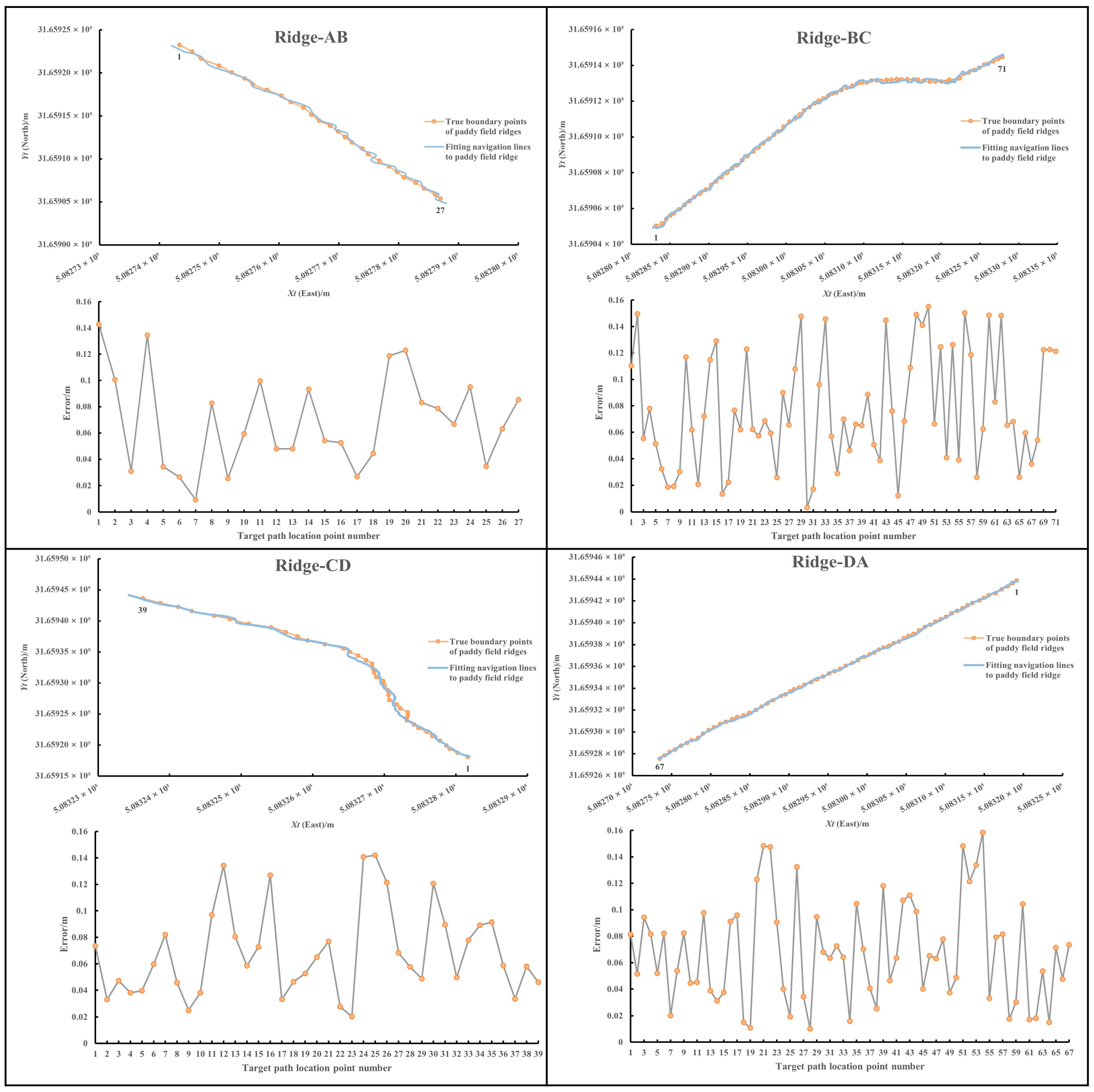
3.2. Navigation Line Coordinate Extraction

In order to verify the accuracy and real-time performance of semantic segmentation and inverse perspective transformation for extracting navigation line coordinates of paddy field ridges, a visual navigation platform for the rice transplanter was built in an actual field for field test verification. The field test environment was a farm paddy field in Shibu Town, Xinjian County, Nanchang City.

The field test process: The rice transplanter traveled along the paddy field ridges. During the test, the rice transplanter was manually operated and kept traveling along the edge rows as much as possible. We ran the program on the Jetson AGX Xavier and acquired the image of the side row in real time using an industrial camera, as shown in Figure 14a,e, and the mask map after model inference, as shown in Figure 14b,f. The AHRS was solidly connected to the industrial camera to obtain camera attitude information, and the MPS-S-1000-V2 was solidly connected to the hydraulic cylinder to obtain camera height information. The communication protocol was customized in STM32, and the AHRS and MPS-S-1000-V2 data frames were packed and sent to AGX so as to carry out inverse perspective transformation and straight-line fitting on the paddy field ridges’ segmented images, as shown in Figure 14c,d,g,h. At the same time, the GNSS acquired the antenna’s positioning information and sent it to the AGX, finally extracted the fitted navigation lines and coordinates of the paddy field ridges using homogeneous coordinate transformation, and printed the process data to the screen and saved it to a Microsoft Excel file.

As shown in Figure 14i, in this study, the manual handheld Sinan’s T300 RTK-GNSS was used to acquire the coordinates of actual paddy field boundary points with an RTK planimetric accuracy of (±8 + 1 × 10⁻⁶ × D) mm, where D represents the distance. Along the paddy field ridges, true boundary points were collected at approximately 1-meter intervals, resulting in a total of 230 boundary points. After the experiment, the extracted navigation line coordinates of the paddy field ridges and the field boundary coordinates measured by RTK-GNSS were plotted in Figure 14.

To verify the accuracy of the extraction of navigation line coordinates of paddy field ridges, the extraction error of navigation line coordinates was analyzed by experimentally comparing the fitted navigation line coordinates of four segments of paddy field ridges (segments AB, BC, CD, and DA, respectively) with the actual field boundary coordinates measured by RTK-GNSS. The error calculation method is as follows: find the nearest point in the extracted navigation line coordinates to the RTK-GNSS-measured field boundary coordinates, and calculate the distance between the two points by the Euclidean distance formula, which is the navigation line coordinate extraction error [42]. The analysis results of the navigation line coordinate extraction error are shown in Figure 15 and

Table 4. Distance error of extracted navigation lines of paddy field ridges.

Ridge	Distance Error (m)
	Maximum	Minimum	Average	Standard Deviation
AB	0.143	0.009	0.069	0.036
BC	0.155	0.003	0.077	0.043
CD	0.142	0.020	0.068	0.033
DA	0.158	0.010	0.068	0.039
Total	0.158	0.003	0.071	0.039

.

The results indicated that the system’s overall average distance error was 0.071 m, with a minimum error of 0.003 m, a maximum error of 0.158 m, and a standard deviation of 0.039 m. The total time required for navigation line extraction was approximately 100 ms.

4. Discussion

This study addressed critical technical challenges associated with autonomous navigation in hilly paddy field environments, including complex topographical variations, irregular boundary distributions, and the limited adaptability of conventional GNSS-based agricultural navigation systems. To mitigate these challenges, a machine vision and GNSS fusion approach was developed for paddy field ridge semantic segmentation and navigation line coordinate extraction. To systematically evaluate the effectiveness of the proposed method in unstructured environments, a comparative analysis was conducted against three representative technical frameworks: (1) a monocular vision-inertial measurement unit (IMU) fusion strategy (inertial-aided); (2) a monocular vision-LiDAR fusion strategy (active perception-driven); and (3) a stereo vision-based strategy (three-dimensional reconstruction-driven).

Wu et al. [14] proposed a monocular vision-IMU fusion framework that integrates the transplanting machine’s pose parameters with navigation parameters through joint calibration, employing an Extended Kalman Filter (EKF) to facilitate vision-inertial data fusion. This approach leverages a lightweight semantic segmentation network to extract the navigation baseline, achieving an average pixel accuracy of 0.984, with a CPU inference time of 0.240 s and a per-frame processing time of 0.392 s. In comparison, although the semantic segmentation model utilized in this study demonstrated a slightly lower average pixel accuracy of 0.924, its deployment was optimized via the TensorRT framework, reducing GPU inference time to 0.038 s and per-frame processing time to 0.1 s, thereby significantly improving real-time performance. Previous studies reported a lateral deviation of 0.044 ± 0.040 m in flat paddy field environments; however, they did not account for deviations in uneven terrain or along curved paths and relied on a fixed camera height parameter. To overcome these limitations, the present study integrates a hydraulic elevation profiling system to dynamically acquire camera height parameters. When combined with a fully calibrated inverse perspective transformation algorithm, this approach enables real-time compensation for both terrain undulations and path curvature variations, ultimately achieving a lateral deviation of 0.071 m. Furthermore, the EKF-based camera pose calibration strategy employed in Wu’s study provided a theoretical foundation for refining the accuracy of navigation line extraction in this research.

He Jing et al. [42] introduced a monocular camera-LiDAR fusion method to facilitate the high-precision extraction of rice row navigation lines through the spatial registration of camera and LiDAR coordinate systems. This method accounts for the influence of an uneven hardpan in paddy fields as well as dynamic variations in vehicle pose, ultimately achieving a maximum lateral deviation of 0.143 m with a standard deviation of 0.043 m. In contrast, the approach presented in this study, which utilized only a monocular camera in conjunction with an inverse perspective transformation technique, achieves a maximum lateral deviation of 0.158 m with a standard deviation of 0.039 m. Nevertheless, in comparison to the machine vision-LiDAR fusion method, the proposed approach demonstrated advantages in terms of lower hardware costs and reduced implementation complexity [40].

Yun et al. [41] developed a binocular stereo-vision system that utilized a stereo camera to capture the three-dimensional structure of the field surface. The system employs a disparity algorithm to dynamically compensate for disturbances in pitch and roll, while also incorporating optical artifact correction to mitigate the effects of environmental light interference. This approach achieves a lateral positioning error of 0.024 m on flat terrain. However, the authors also highlighted that the method relies on conventional image processing workflows, which render the binocular camera vulnerable to strong light reflections and motion-induced jitter, thereby increasing the failure rate of feature matching. Furthermore, the high computational complexity and limited real-time performance [42] restrict the operational speed of the experimental vehicle to 0.25 m/s. In contrast, the current study integrated a lightweight semantic segmentation model, an enhanced, noise-resistant dataset, and an adaptive inverse perspective mapping (IPM) correction algorithm to effectively mitigate the coupled disturbances arising from uneven terrain and nonlinear boundaries. Additionally, by incorporating GNSS absolute positioning data, the proposed system significantly enhances overall robustness, while demonstrating considerable advantages in terms of computational efficiency, cost-effectiveness, and adaptability.

Regarding technical applicability, the multi-sensor fusion framework developed in this study demonstrates a significant capacity for cross-scenario adaptation, thereby rendering it suitable for deployment in various agricultural environments, such as dryland fields and orchards. In dryland contexts, despite the high coverage of GNSS signals and the method’s ability to adapt to variations in soil texture, factors such as humidity gradients, crop residue, and lighting heterogeneity may lead to a decline in the performance of semantic segmentation, thus necessitating further optimization of the visual feature extraction module. In orchard environments, the challenges posed by GNSS signal obstruction due to tree canopies and multipath interference [13] are mitigated by utilizing deep learning-driven relative positioning and comprehensive inverse perspective mapping (IPM) correction. This combination provides high-precision coordinate references for the integration of visual SLAM (Simultaneous Localization and Mapping) and odometry, thereby ensuring stable navigation performance in signal-constrained environments.

However, the study is subject to certain limitations:

(1)

Constraints in Data-Driven Generalization: The limited availability of open benchmark datasets for agricultural environments presents a substantial challenge. The self-constructed paddy field dataset exhibits constraints in both sample size and environmental diversity [32]. To address these limitations, future research will focus on developing a heterogeneous agricultural scene dataset through data acquisition across multiple regions and climatic conditions. Furthermore, the integration of self-supervised learning and domain adaptation techniques will be explored to minimize dependence on manual annotations and enhance the model’s generalization capabilities.

(2)

Navigation Integrity in Complex Environments: Effective field path planning and autonomous navigation for rice transplanters necessitate improved detection and localization of field headlands, facilitating precise distance estimation between the transplanter and the headland to enable automated turning maneuvers. Achieving this objective requires the refinement of the transplanter-to-headland distance estimation model, the development of autonomous steering control algorithms, and the online calibration of system parameters. Future investigations will integrate an extended Kalman filter (EKF) within a multi-sensor data fusion framework, with the system’s performance validated through autonomous field navigation experiments.

(3)

Challenges in Energy-Efficiency Optimization: The high computational demands of the Jetson AGX Xavier platform are accompanied by substantial energy consumption, constraining its deployment in resource-limited agricultural machinery. To mitigate this issue, subsequent research will prioritize algorithm optimization for computational efficiency, hardware acceleration (e.g., NVIDIA Jetson Xavier NX), and dynamic load scheduling strategies to achieve a balanced trade-off between system performance and energy efficiency across diverse operational scenarios.

5. Conclusions

In this study, we proposed a method for extracting the navigation line coordinates of paddy field ridges based on machine vision fused with GNSS. First, we constructed a real-time semantic segmentation model for extracting the mask map of paddy field ridges. Second, we designed a multi-sensor fusion method combining the AHRS and a hydraulic elevation profiling device to dynamically acquire the camera’s external parameters to improve inverse perspective transformation and obtain a bird’ s-eye view. Finally, we used homogeneous coordinate transformation to obtain navigation line coordinate information and deployed the model and algorithm on the Jetson AGX Xavier embedded development board to realize the real-time segmentation and extraction of navigation line coordinates of paddy field ridges, which provided important navigation coordinate information for the rice transplanter’s navigation control system. The main research conclusions are as follows:

(1)

To overcome the difficulty in extracting complex paddy field boundary information in hilly areas and the limitation in applying GNSS agricultural navigation, a semantic segmentation network was used to extract the paddy field boundary, and a paddy field ridge image dataset and a BiSeNet semantic segmentation model were constructed. The model training and testing results showed that the model’s pixel accuracy is 92.61%, the average intersection and merger ratio is 90.88%, and the model segmentation speed is up to 18.87 fps. In addition, we deployed the model on the Jetson AGX Xavier embedded development platform and optimized the BiSeNet model deployment using the TensorRT model inference framework. The experimental data showed that the optimized model deployment using TensorRT with FP16 data accuracy and a 1024 × 1024 model image input size had the best performance, with a real-time model segmentation speed of 26.31 fps, an average intersection and merger ratio of 90.62%, and a model pixel segmentation accuracy of 92.43%, which meets the requirements of the real-time segmentation of paddy field ridges in terms of speed and accuracy.

(2)

Since existing navigation line extraction techniques lack high-precision coordinate localization to support global path planning, we proposed a method that combines inverse perspective transformation and homogeneous coordinate transformation to accurately and reliably extract the navigation line coordinates of paddy field ridges. As inverse perspective transformation is not applicable to the unevenness of the hard bottom layer of paddy fields, we obtained the camera’s 3D attitude angle through the AHRS and designed a method and device to measure the height of the rice transplanter’s on-board camera from paddy fields based on a hydraulic profiling system so as to obtain the camera’s dynamic external parameter and improve the inverse perspective transformation.

(3)

The proposed method was realized on a rice transplanter, and tests were carried out in the actual field. The accuracy and real-time performance of the method for paddy field segmentation and navigation line coordinate extraction were verified by calculating the distance error between the fitted navigation line of the paddy field ridges and their real boundary. The test results showed that the average distance error is 0.071 m, the standard deviation is 0.039 m, and the overall time consumed is about 100 ms, which basically meets the accuracy and real-time requirements of navigation line extraction under a rice transplanter operation speed of 0.7 m s⁻¹.

References

- Khadatkar, A.; Mathur, S.M.; Dubey, K.; BhusanaBabu, V. Development of Embedded Automatic Transplanting System in Seedling Transplanters for Precision Agriculture. Artif. Intell. Agric. 2021, 5, 175–184. [Google Scholar] [CrossRef]
- Duckett, T.; Pearson, S.; Blackmore, S.; Grieve, B.; Chen, W.-H.; Cielniak, G.; Cleaversmith, J.; Dai, J.; Davis, S.; Fox, C.; et al. Agricultural Robotics: The Future of Robotic Agriculture. arXiv 2018, arXiv:1806.06762. Available online: https://arxiv.org/abs/1806.06762 (accessed on 18 January 2024).
- Reddy Maddikunta, P.K.; Hakak, S.; Alazab, M.; Bhattacharya, S.; Gadekallu, T.R.; Khan, W.Z.; Pham, Q.-V. Unmanned Aerial Vehicles in Smart Agriculture: Applications, Requirements, and Challenges. IEEE Sens. J. 2021, 21, 17608–17619. [Google Scholar] [CrossRef]
- Varotsos, C.A.; Cracknell, A.P. Remote Sensing Letters Contribution to the Success of the Sustainable Development Goals—N 2030 Agenda. Remote Sens. Lett. 2020, 11, 715–719. [Google Scholar] [CrossRef]
- Idoje, G.; Dagiuklas, T.; Iqbal, M. Survey for Smart Farming Technologies: Challenges and Issues. Comput. Electr. Eng. 2021, 92, 107104. [Google Scholar] [CrossRef]
- Bechar, A.; Vigneault, C. Agricultural Robots for Field Operations. Part 2: Operations and Systems. Biosyst. Eng. 2017, 153, 110–128. [Google Scholar] [CrossRef]
- dos Santos, A.F.; da Silva, R.P.; Zerbato, C.; de Menezes, P.C.; Kazama, E.H.; Paixão, C.S.S.; Voltarelli, M.A. Use of Real-Time Extend GNSS for Planting and Inverting Peanuts. Precis. Agric. 2019, 20, 840–856. [Google Scholar] [CrossRef]
- Meng, Z.; Wang, H.; Fu, W.; Liu, M.; Yin, Y.; Zhao, C. Research Status and Prospects of Agricultural Machinery Autonomous Driving. Trans. Chin. Soc. Agric. Mach. 2023, 54, 1–24. [Google Scholar] [CrossRef]
- Zhou, J.; He, Y. Research Progress on Navigation Path Planning of Agricultural Machinery. Trans. Chin. Soc. Agric. Mach. 2021, 52, 1–14. [Google Scholar] [CrossRef]
- Zhang, H.; He, B.; Xing, J. Mapping Paddy Rice in Complex Landscapes with Landsat Time Series Data and Superpixel-Based Deep Learning Method. Remote Sens. 2022, 14, 3721. [Google Scholar] [CrossRef]
- Xie, B.; Jin, Y.; Faheem, M.; Gao, W.; Liu, J.; Jiang, H.; Cai, L.; Li, Y. Research Progress of Autonomous Navigation Technology for Multi-Agricultural Scenes. Comput. Electron. Agric. 2023, 211, 107963. [Google Scholar] [CrossRef]
- Bai, Y.; Zhang, B.; Xu, N.; Zhou, J.; Shi, J.; Diao, Z. Vision-Based Navigation and Guidance for Agricultural Autonomous Vehicles and Robots: A Review. Comput. Electron. Agric. 2023, 205, 107584. [Google Scholar] [CrossRef]
- Wu, W.; Zhang, Z.; Zhang, X.; He, Y.; Fang, H. Application of Visual Inertia Fusion Technology in Rice Transplanter Operation. Comput. Electron. Agric. 2024, 221, 108990. [Google Scholar] [CrossRef]
- Alsalam, B.H.Y.; Morton, K.; Campbell, D.; Gonzalez, F. Autonomous UAV with Vision Based On-Board Decision Making for Remote Sensing and Precision Agriculture. In Proceedings of the 2017 IEEE Aerospace Conference, Big Sky, MT, USA, 4–11 March 2017; pp. 1–12. [Google Scholar]
- Adhikari, S.P.; Kim, G.; Kim, H. Deep Neural Network-Based System for Autonomous Navigation in Paddy Field. IEEE Access 2020, 8, 71272–71278. [Google Scholar] [CrossRef]
- Sevak, J.S.; Kapadia, A.D.; Chavda, J.B.; Shah, A.; Rahevar, M. Survey on Semantic Image Segmentation Techniques. In Proceedings of the 2017 International Conference on Intelligent Sustainable Systems (ICISS), Palladam, Thirupur, India, 7–8 December 2017; pp. 306–313. [Google Scholar]
- Alsaeed, D.; Bouridane, A.; El-Zaart, A. A Novel Fast Otsu Digital Image Segmentation Method. Int. Arab. J. Inf. Technol. 2016, 13, 427–434. [Google Scholar]
- Wang, Q.; Liu, H.; Yang, P.; Meng, Z. Detection Method of Headland Boundary Line Based on Machine Vision. Trans. Chin. Soc. Agric. Mach. 2020, 51, 18–27. [Google Scholar]
- Pandey, R.; Lalchhanhima, R. Segmentation Techniques for Complex Image: Review. In Proceedings of the 2020 International Conference on Computational Performance Evaluation (ComPE), Shillong, India, 2–4 July 2020; pp. 804–808. [Google Scholar]
- Li, Y.; Hong, Z.; Cai, D.; Huang, Y.; Gong, L.; Liu, C. A SVM and SLIC Based Detection Method for Paddy Field Boundary Line. Sensors 2020, 20, 2610. [Google Scholar] [CrossRef]
- Jafari, M.H.; Samavi, S. Iterative Semi-Supervised Learning Approach for Color Image Segmentation. In Proceedings of the 2015 9th Iranian Conference on Machine Vision and Image Processing (MVIP), Tehran, Iran, 18–19 November 2015; pp. 76–79. [Google Scholar]
- Jiang, Q.; Fang, S.; Peng, Y.; Gong, Y.; Zhu, R.; Wu, X.; Ma, Y.; Duan, B.; Liu, J. UAV-Based Biomass Estimation for Rice-Combining Spectral, TIN-Based Structural and Meteorological Features. Remote Sens. 2019, 11, 890. [Google Scholar] [CrossRef]
- Trebing, K.; Staǹczyk, T.; Mehrkanoon, S. SmaAt-UNet: Precipitation Nowcasting Using a Small Attention-UNet Architecture. Pattern Recognit. Lett. 2021, 145, 178–186. [Google Scholar] [CrossRef]
- He, Y.; Zhang, X.; Zhang, Z.; Fang, H. Automated Detection of Boundary Line in Paddy Field Using MobileV2-UNet and RANSAC. Comput. Electron. Agric. 2022, 194, 106697. [Google Scholar] [CrossRef]
- Liu, X.; Qi, J.; Zhang, W.; Bao, Z.; Wang, K.; Li, N. Recognition Method of Maize Crop Rows at the Seedling Stage Based on MS-ERFNet Model. Comput. Electron. Agric. 2023, 211, 107964. [Google Scholar] [CrossRef]
- Choi, K.H.; Han, S.K.; Han, S.H.; Park, K.-H.; Kim, K.-S.; Kim, S. Morphology-Based Guidance Line Extraction for an Autonomous Weeding Robot in Paddy Fields. Comput. Electron. Agric. 2015, 113, 266–274. [Google Scholar] [CrossRef]
- Chen, J.; Qiang, H.; Wu, J.; Xu, G.; Wang, Z. Navigation Path Extraction for Greenhouse Cucumber-Picking Robots Using the Prediction-Point Hough Transform. Comput. Electron. Agric. 2021, 180, 105911. [Google Scholar] [CrossRef]
- Fu, D.; Jiang, Q.; Qi, L.; Xing, H.; Chen, Z.; Yang, X. Detection of the centerline of rice seedling belts based on region growth sequential clustering-RANSAC. Trans. CSAE 2023, 39, 47–57. [Google Scholar] [CrossRef]
- Fragoso, V.; Sweeney, C.; Sen, P.; Turk, M. ANSAC: Adaptive Non-Minimal Sample and Consensus. arXiv 2017, arXiv:1709.09559. Available online: https://arxiv.org/abs/1709.09559 (accessed on 21 November 2024).
- Diao, Z.; Guo, P.; Zhang, B.; Zhang, D.; Yan, J.; He, Z.; Zhao, S.; Zhao, C. Maize Crop Row Recognition Algorithm Based on Improved UNet Network. Comput. Electron. Agric. 2023, 210, 107940. [Google Scholar] [CrossRef]
- Wang, T.; Chen, B.; Zhang, Z.; Li, H.; Zhang, M. Applications of Machine Vision in Agricultural Robot Navigation: A Review. Comput. Electron. Agric. 2022, 198, 107085. [Google Scholar] [CrossRef]
- Hong, Z.; Li, Y.; Lin, H.; Gong, L.; Liu, C. Field Boundary Distance Detection Method in Early Stage of Planting Based on Binocular Vision. Field Boundary Distance Detection Method. in Early Stage of Plantin Based on Binocular Vision. Trans. Chin. Soc. Agric. Mach. 2022, 53, 27–33+56. [Google Scholar]
- Masiero, A.; Sofia, G.; Tarolli, P. Quick 3D With UAV and TOF Camera For Geomorphometric Assessment. In Proceedings of the The International Archives of the Photogrammetry, Remote Sensing and Spatial Information Sciences, Nice, France, 31 August–2 September 2020; XLIII-B1. pp. 259–264. [Google Scholar] [CrossRef]
- Ji, Y.; Xu, H.; Zhang, M.; Li, S.; Cao, R.; Li, H. Design of Point Cloud Acquisition System for Farmland Environment Based on LiDAR. Trans. Chin. Soc. Agric. Mach. 2019, 50, 1–7. [Google Scholar]
- Wang, S.; Song, J.; Qi, P.; Yuan, C.; Wu, H.; Zhang, L.; Liu, W.; Liu, Y.; He, X. Design and Development of Orchard Autonomous Navigation Spray System. Front. Plant Sci. 2022, 13, 960686. [Google Scholar] [CrossRef]
- Liu, H.; Li, Y.; Liu, Z.; Huang, F.; Liu, C. Rice Rows Detection and Navigation Information Extraction Method—Based on Camera Pose. J. Agric. Mech. Res. 2024, 46, 15–21. [Google Scholar] [CrossRef]
- Zhang, S.; Wang, Y.; Zhu, Z.; Li, Z.; Du, Y.; Mao, E. Tractor Path Tracking Control Based on Binocular Vision. Inf. Process. Agric. 2018, 5, 422–432. [Google Scholar] [CrossRef]
- Yu, C.; Wang, J.; Peng, C.; Gao, C.; Yu, G.; Sang, N. BiSeNet: Bilateral Segmentation Network for Real-Time Semantic Segmentation. In Proceedings of the European Conference on Computer Vision (ECCV), Munich, Germany, 8–14 September 2018; pp. 325–341. [Google Scholar] [CrossRef]
- He, K.; Zhang, X.; Ren, S.; Sun, J. Deep Residual Learning for Image Recognition. In Proceedings of the 2016 IEEE Conference on Computer Vision and Pattern Recognition (CVPR), Las Vegas, NV, USA, 27–30 June 2016; pp. 770–778. [Google Scholar]
- Aly, M. Real Time Detection of Lane Markers in Urban Streets. In Proceedings of the 2008 IEEE Intelligent Vehicles Symposium, Eindhoven, The Netherlands, 4–6 June 2008; pp. 7–12. [Google Scholar]
- Zhang, Z. A Flexible New Technique for Camera Calibration. IEEE Trans. Pattern Anal. Mach. Intell. 2000, 22, 1330–1334. [Google Scholar] [CrossRef]
- He, J.; He, J.; Luo, X.; Li, W.; Man, Z.; Feng, D. Rice Row Recognition and Navigation Control Based on Multi-sensor Fusion. Trans. Chin. Soc. Agric. Mach. 2022, 53, 18–26+137. [Google Scholar] [CrossRef]