Soybean–Corn Seedling Crop Row Detection for Agricultural Autonomous Navigation Based on GD-YOLOv10n-Seg

Abstract

Accurate crop row detection is an important foundation for agricultural machinery to realize autonomous operation. Existing methods often compromise between real-time performance and detection accuracy, limiting their practical field applicability. This study develops a high-precision, efficient crop row detection algorithm specifically optimized for soybean–corn compound planting conditions, addressing both computational efficiency and recognition accuracy. In this paper, a real-time soybean–corn crop row detection method based on GD-YOLOv10n-seg with principal component analysis (PCA) fitting was proposed. Firstly, the dataset of soybean–corn seedling crop rows was established, and the images were labeled with line labels. Then, an improved model GD-YOLOv10n-seg model was constructed by integrating GhostModule and DynamicConv into the YOLOv10n-segmentation model. The experimental results showed that the improved model performed better in MPA and MIoU, and the model size was reduced by 18.3%. The crop row center lines of the segmentation results were fitted by PCA, where the fitting accuracy reached 95.08%, the angle deviation was 1.75°, and the overall processing speed was 61.47 FPS. This study can provide an efficient and reliable solution for agricultural autonomous navigation operations such as weeding and pesticide application under a soybean–corn compound planting mode.

1. Introduction

In 2022, China began to promote soybean–corn compound planting. Soybean–corn compound planting can effectively alleviate the pressure of soybean and corn production shortage [1]. It is of great significance to develop autonomous agricultural machinery suitable for the soybean–corn compound planting mode to improve field work efficiency and reduce labor demand and the production cost. The autonomous navigation of agricultural machinery is an important part of agricultural autonomous operation, which has always been a concern in the field of intelligent agriculture. The research on the autonomous navigation of agricultural machinery can be traced back to the 1980s [2]. Autonomous navigation has the potential to reduce the reliance on manual labor in field work and enhance work precision according to the authors of [3]. In recent years, intelligent agriculture has witnessed notable development. However, autonomous navigation in agricultural machinery remains at an early stage of development and many issues relating to it remain unresolved [4]. The main challenge is to strike a balance between ensuring navigation accuracy and maintaining timeliness.

The global navigation satellite system (GNSS) is widely used in autonomous navigation of agricultural machinery [5]. The GNSS provides centimeter-level positioning accuracy, which is sufficient for many agricultural operations. However, its application requires machinery to follow predefined paths and record absolute coordinates during operation. This approach does not support real-time acquisition of the relative position between the machinery and the crop rows, thereby limiting the flexibility of steering control. At the same time, as the actual growth position of crops sometimes changes in a semi-structured environment, operating according to a fixed path may cause some crops to be crushed [6]. In addition, as field management operations such as weeding and spraying are developing in a precise direction, it will be more necessary to obtain the relative posture between the machine and the crop [7].

In order to solve the problem that the GNSS cannot obtain the relative position between machines and crops, cameras and lidars have been widely applied to obtain the position information of farmland crops and support the autonomous navigation of agricultural machinery. The working principle of lidar is to send a signal to the target, compare the returned target echo with the transmitted signal to obtain more target information, and use this information to directly calculate the distance between the lidar and the reflecting target [8]. Lidar can provide a three-dimensional environmental awareness, providing not only the distance to the target but also the height and shape information of the target which can help the agricultural machinery accurately perceive and identify obstacles, plants, and terrain in farmland [9]. Although lidar has the advantages of high precision and reliability in farmland navigation, it also has some disadvantages, such as a high use cost and complex data processing [10,11].

A visual processing system can be used to acquire the images of the crop rows, calculate the course deviation between the agricultural machinery and crop rows through algorithms, and convert it into real-time steering control signals. Compared to the GNSS, using the visual processing system eliminates the need for pre-acquiring the travel path. An increasing number of studies recognize the importance of the vision processing system in autonomous navigation due to its low cost, high flexibility, and strong data processing capabilities [12]. As a result, the vision processing system has gradually become one of the main technical solutions for the autonomous navigation of agricultural machinery [13,14]. For example, the AgBot II [15] intelligent weeding robot developed by Queensland University of Science and Technology in Australia, the Dino15 robot developed in France, the AVO [16] weeding robot developed by the Swiss company ecoRobotix, and the HortiBot [17] weeding robot developed by the Agricultural Research Institute of Aarhus University in Denmark. These robots all adopt a vision processing system to accurately identify crops and weeds, thus realizing navigation control and weeding operations. Although the unstructured field environment usually has a negative impact on the information collected by cameras, the vision-based navigation system has great advantages in terms of its low cost, timeliness, information processing richness, and expandability [18]. The vision-based navigation technologies are mainly divided into two categories: traditional image processing methods and deep learning-based image processing methods. Among the traditional methods, improved color threshold segmentation techniques are widely used for crop and soil background segmentation [19,20,21], and then the feature extraction is carried out to identify the navigation lines. In order to identify the corn seedlings and the weeds effectively in the field, Montalvo et al. (2012) adopted a dual-threshold segmentation method, significantly reducing the impact of weeds on crop row segmentation and achieving accurate crop row detection [22]. Yue Yu et al. (2021) applied a triple classification method to segment rice seedlings and a two-dimensional adaptive clustering method to eliminate misleading crop feature points [23]. The experimental results demonstrated that this method could obtain a satisfactory extraction effect for navigation lines even in a complex paddy field environment where weeds were overgrown. Leemans et al. (2006) enhanced the applicability of the classical Hough transform, enabling effective background segmentation and crop row extraction even in extremely noisy environments where some crop rows are a lack of plants [24]. Although these traditional image processing methods are effective in certain cases, they are easily affected by the noise from lighting conditions and weeds, resulting in poor anti-interference capabilities. This may lead to a decrease in the detection accuracy and robustness in semi-structured field environments.

In recent years, deep learning has made great progress across various domains, including autonomous driving, image processing, speech recognition, etc. Notably, the application of transfer learning has addressed the critical challenge of limited domain-specific datasets in the agricultural sector [25,26,27]. It is most commonly used in crop identification [28], weed identification [29], plant pest detection [30], and agricultural robot navigation in the field of agricultural engineering. In order to reduce the complexity of traditional image segmentation, many researchers use semantic segmentation technology to detect crop rows [31]. Adhikari SP et al. (2020) established a rice rows segmentation method based on the ES-Net network model and used the sliding window algorithm to cluster and fit crop rows in the region of interest (ROI) [32]. The geometric median line formed by the last two crop rows was used as the navigation line. In order to adapt to the different row spacing of strawberries, Ponnambalam et al. (2020) used SegNet to identify and segment strawberry crop rows, and used an adaptive ROI algorithm to realize the autonomous navigation of strawberries with different row spacing [33]. Bah et al. (2020) proposed a CRowNet model composed of SegNet and Hough transform which was used to detect the crop rows in the images taken by unmanned aerial vehicles and realized the effective extraction of crop rows [34]. In addition to segmentation algorithms, target detection algorithms based on deep learning are also used to extract crop rows. These algorithms generally detect the target crops and then process them according to their position information to generate crop rows. Ruan et al. (2023) used the YOLO-R algorithm to detect crops in the field and used the DBSCAN clustering algorithm to generate crop rows, thus accurately estimating the number of crop rows in an image and the number of crops in each row [35]. Gong et al. (2024) used the YOLOX algorithm to detect corn in a field and used the least square method to fit crop rows [36]. The existing research on crop row detection shows that the traditional computer vision technology is insufficient in accurately predicting crop rows under different field conditions, and the methods based on deep learning have been proven to produce robust crop row detection methods under different field conditions. Crop row detection serves as the foundational step toward achieving autonomous navigation. Following the acquisition of the crop row mask, post-processing is required to extract precise information regarding the crop row lines. Although the deep learning algorithm can generate reliable crop row mask or crop position information based on the input image, it still needs a robust algorithm to generate the crop row lines.

At present, semantic segmentation and target detection algorithms have been widely used in the research work of crop row detection, and they have achieved good detection results which provides guidance for the work of this paper. The aim of this study is to further develop the intelligent detection of crop rows by using an improved YOLOv10n-segmentation algorithm to synchronize the generation of crop row masks as well as positional information, thus enabling the fast fitting of crop row lines while reducing the model parameters. The main work is as follows:

(1)

Establishing a field crop row image dataset under the soybean–corn compound planting mode;

(2)

Establishing a crop row segmentation model of soybean–corn crop rows based on the improved YOLOv10n-segmentation algorithm;

(3)

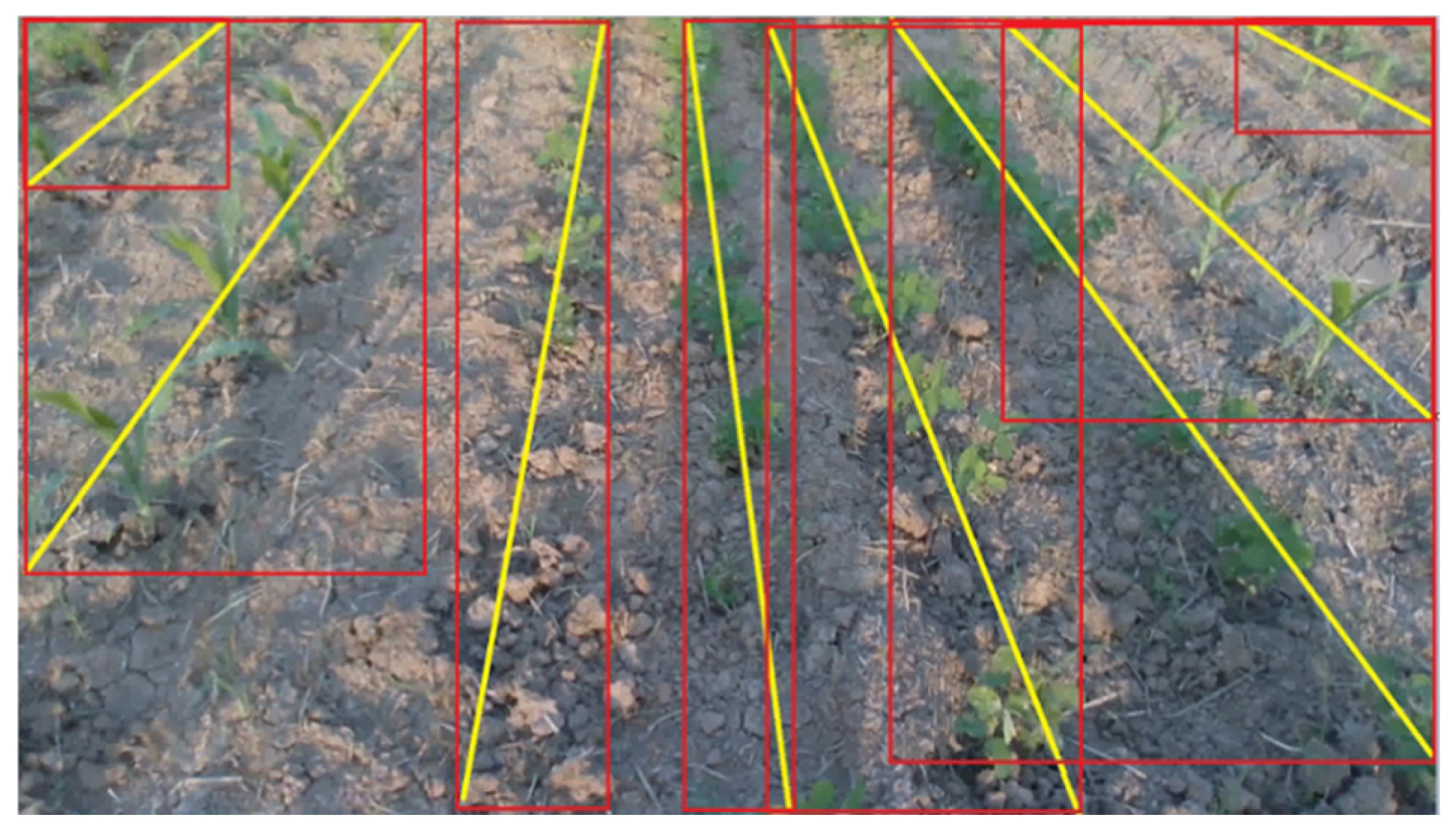
Generating the crop row lines based on the segmentation results;

(4)

Testing the accuracy of the crop row line generation results.

2. Materials and Methods

This study proposes a method for extracting soybean–corn crop row lines using a two-step process: (1) crop row detection and (2) crop row line fitting. Detection is performed using an improved segmentation model named GD-YOLOv10n-seg, which operates at the pixel level to generate segmentation masks of each crop row. These masks are then processed using a PCA-based algorithm to fit straight crop row lines. The overall workflow is illustrated in Figure 1.

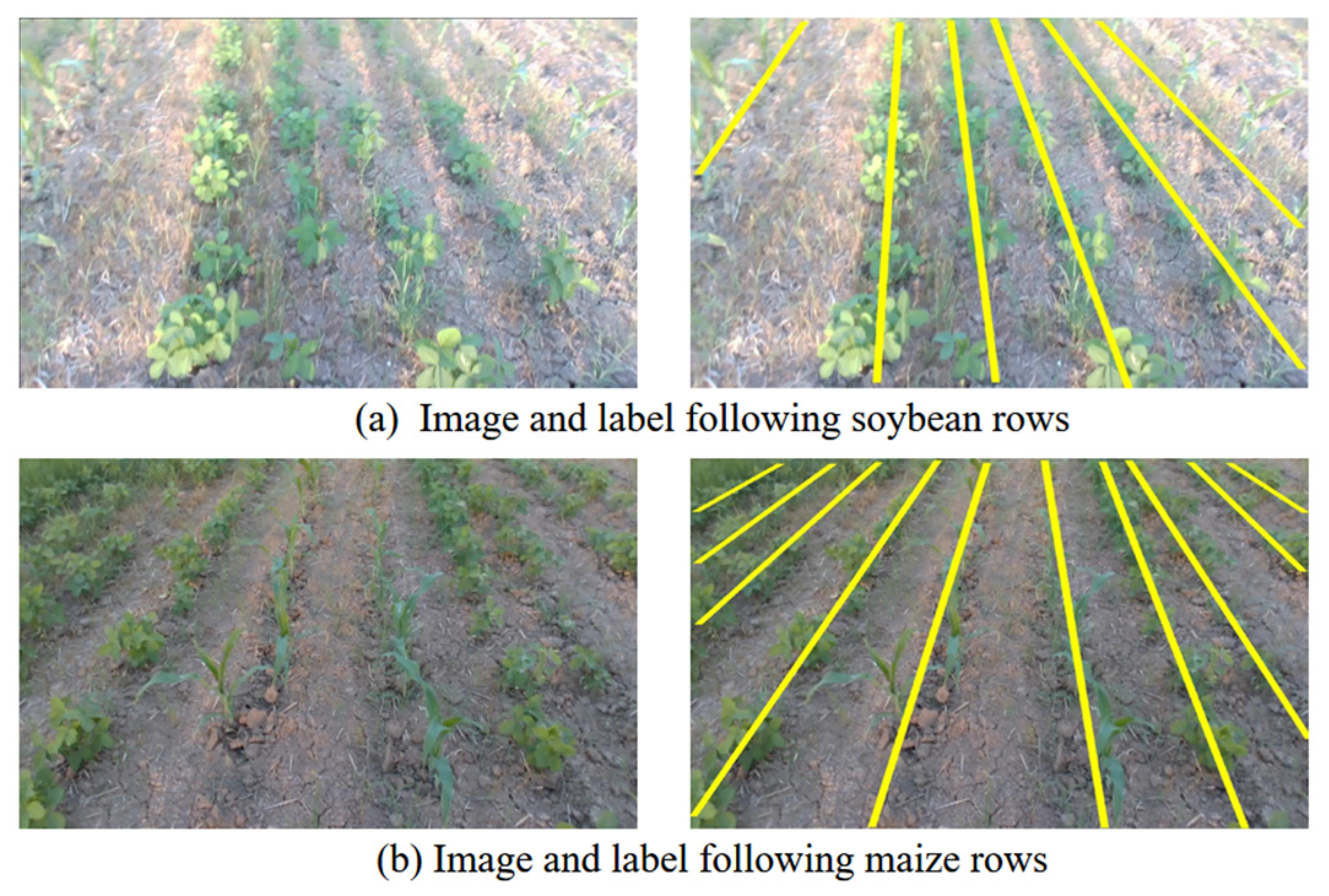
2.1. Image Acquisition and Dataset Construction

A custom image dataset was constructed to capture soybean–corn compound planting at the seedling stage. Images were acquired using the NJS-4D4S field management robotic platform (NIAM, Nanjing, China), equipped with an Intel RealSense D435i depth camera (Microsoft, Redmond, WA, USA). The camera was mounted at 150 cm height with a 30° downward angle and captured RGB images with a resolution of 1920 × 720 pixels.

The first part of the dataset was collected on 25 June 2023 in Gunnan County, Lianyungang City, Jiangsu Province, China, and the second part of the dataset was collected on 5 July 2023 in Suining County, Xuzhou City, Jiangsu Province, China. A total of 1500 images of crop rows under different weather conditions, different environmental backgrounds, and different light intensities were collected, and the dataset included images traveling along the corn crop rows as well as those traveling along the soybean crop rows, which were used to simulate the conditions during the actual field operation. We selected the seedling stage for dataset collection and model development because the crop rows are clearly distinguishable during this period. In later growth stages, corn and soybean plants tend to overlap and canopy closure occurs, making it more difficult to accurately identify individual crop rows.

LabelMe (v3.16.7, MIT CSAIL) was used for manual annotation. Instead of traditional polygon masks, we employed line-based labeling with a fixed line width of 24 pixels to approximate the real crop row width. All crop rows, regardless of crop type, were uniformly labeled as “croprow.” Figure 2 shows an example of the raw and annotated images. The dataset was split 8:2 into a training set (1200 images) and a validation set (300 images).

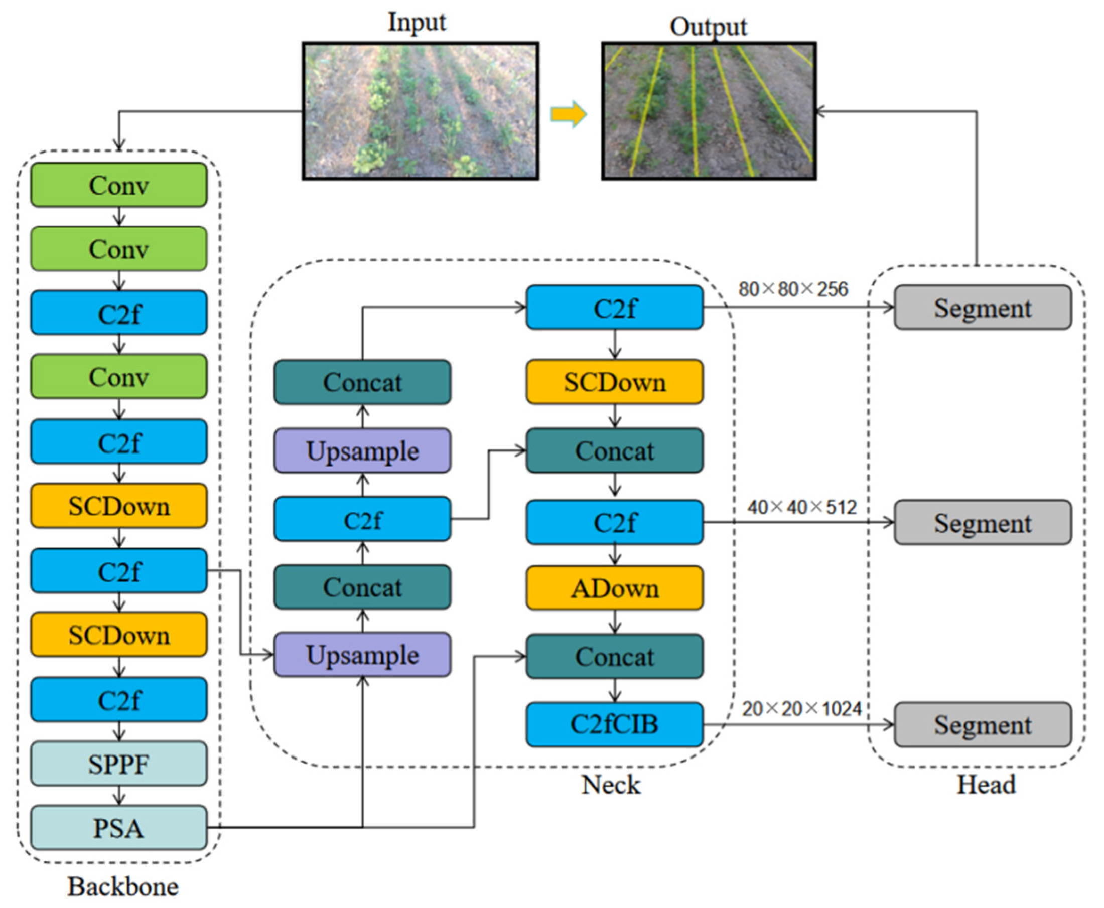
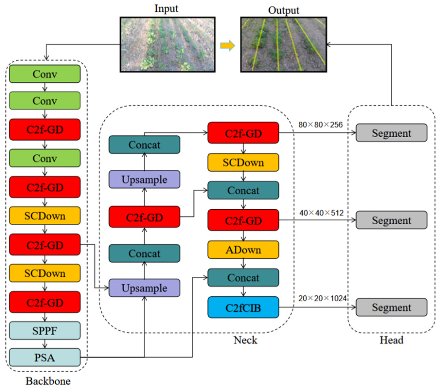
2.2. Crop Row Detection Model

Real-time performance is critical for crop row extraction, which mainly depends on the fast detection of crop rows. Commonly used deep learning-based crop row detection methods can be divided into two methods, semantic segmentation and target detection, both of which have their own advantages. The semantic segmentation-based crop row detection method can directly identify the outline of the crop row and be used for subsequent crop row line fitting operations, while the target detection-based crop row detection method mainly identifies the crop plants and generates the crop row line by connecting the centroid of the plants in post-processing. The former method can detect crop rows with high accuracy and the extraction of crop row lines is also direct and simple, whilst the latter has a higher detection speed but needs to process the results to obtain the crop row lines: both algorithms have a wide range of applications.

In agricultural applications, especially crop row detection and mechanical navigation systems, the real-time performance is extremely critical. Instance segmentation algorithms, while providing more detailed object recognition and segmentation, tend to require more computational resources and processing time due to their higher complexity [37]. These algorithms require the independent prediction of boundaries and masks for each detected object, which undoubtedly increases the computational effort. The processor arithmetic power carried by the agricultural machinery tends to be low and requires longer processing time when running complex models, and the use of instance segmentation algorithms for crop row detection can adversely affect the real-time performance. Therefore, few instance segmentation algorithms have been used for applications in agriculture.

The YOLO algorithm, as a classical target detection algorithm with high detection speed, has made a major breakthrough in real-time performance whilst ensuring detection accuracy. With the development of the algorithm, the network structure and performance of YOLO are increasingly enhanced. In YOLOv5 and later versions, the instance segmentation function is added to the output layer of YOLO, which makes YOLO not only be used to perform target detection but also achieve high-speed instance segmentation.

YOLOv10n-seg was selected as the baseline due to the following advantages:

(1)

Real-time performance: YOLOv10 is a new real-time target detection method developed by researchers at Tsinghua University that addresses the shortcomings of previous versions of YOLO in terms of post-processing and model architecture. By eliminating non-maximum suppression (NMS) and optimizing various model components, YOLOv10 achieves high recognition performance while significantly reducing computational consumption [38].

(2)

Lightweight design: Considering the requirement of reducing computational consumption in resource-constrained environments, we chose YOLOv10n-segmentation (YOLOv10n-seg) as the baseline algorithm. This model has the smallest number of parameters and GFlops among the YOLOv10 algorithms, allowing it to significantly reduce computational consumption while maintaining high performance.

(3)

Segmentation capability: YOLOv10n-seg integrates instance segmentation functionality, allowing for the direct generation of crop row masks without additional post-processing steps. When performing instance segmentation operations, YOLOv10n-seg first detects objects using a target detector and then passes the detected objects to the instance segmentation detector to generate a segmentation mask for each object. This approach not only identifies the location of the objects but also obtains their exact shapes, which effectively improves the speed of the segmentation, resulting in a high real-time performance.

The network structure and basic modules of YOLOv10n-seg are shown in Figure 3. The network structure, the backbone, and the neck module of YOLOv10n-seg are identical to the YOLOv10n target detection algorithm, and an extra detector for segmentation is added alongside the original detector.

2.2.1. Label Visualization

After line labeling was completed, the labeled images input into the YOLOv10n-seg model were subjected to both segmentation and object detection operations, with the label for segmentation being a straight line along the crop row and the label for object detection being the smallest outer quadrilateral of the segment label, as shown in Figure 4. From the labeling diagram, we can find that the crop rows in the image are not parallel to each other due to the camera’s perspective principle [39].

The labels were saved in txt format, which contained the numerical labels of crow rows and the normalized values of the contour vertex coordinates of each line with respect to the size of the original image.

Object detection labels were automatically generated as minimal bounding rectangles enclosing the 24-pixel-wide line annotations, serving dual purposes:

(1)

Providing region proposals for the segmentation head;

(2)

Constraining mask predictions within biologically plausible areas.

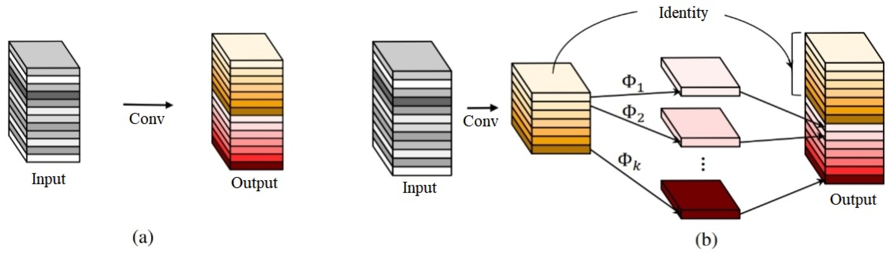
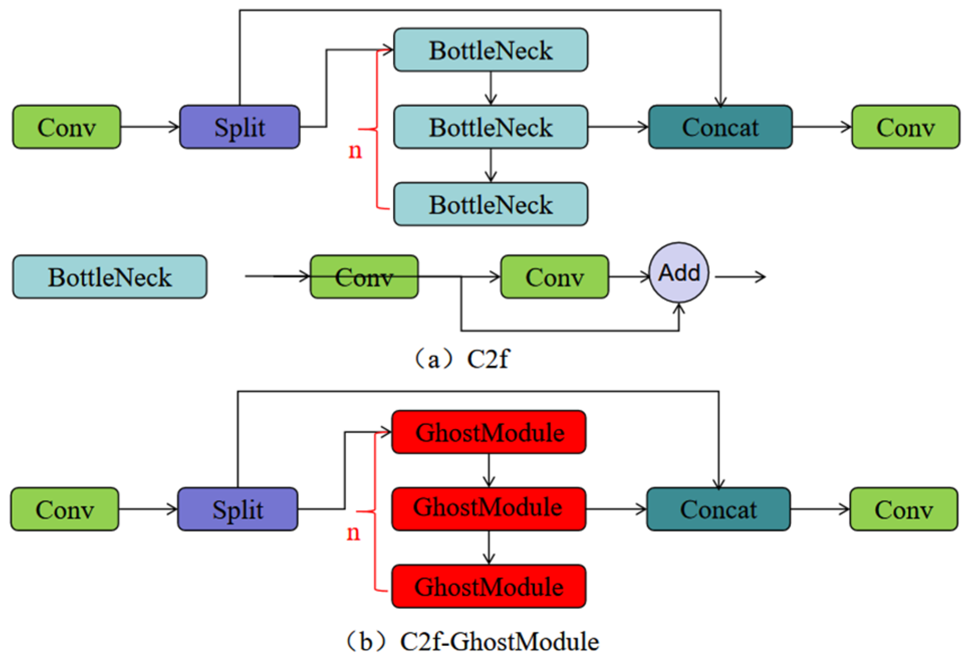
2.2.2. C2f Improvements Based on GhostModule

YOLOv10, like the YOLOv8 algorithm, uses the C2f module (faster implementation of CSP Bottleneck with 2 convolutions). The C2f module improves the multi-scale information extraction by combining convolutions and multiple bottlenecks. As the number of network layers increases, the number of feature maps per channel also increases. When processing feature maps for multiple channels, each channel may contain similar or identical information, leading to a potential redundancy. There are multiple C2f modules in YOLOv10n-seg, and lightweight improvements to these modules can reduce the computational burden and thus enhance the deployment capability of the model.

GhostModule, a lightweight module proposed by GhostNet [40], is widely used in various deep learning models [41,42,43]. The main goal of GhostModule is to use less computational resources to generate the same number of feature maps as the traditional convolutional operations. In GhostModule (Figure 5), the standard convolution operation is first performed using fewer convolution kernels, which generates fewer feature maps. From the base feature maps generated in the first step, GhostModule applies a cheap operation to generate more ghost feature maps. Ghost feature maps are designed to increase the number of feature maps by copying or slightly modifying them from the base feature maps through cheap operations rather than by performing a complete convolution. Finally, the two parts of the feature maps are stitched into a complete feature map through the concat operation. These operations are computationally inexpensive but effective in increasing the number of feature maps and thus enhancing the expressive power of the network.

The equation for the flops of the ordinary convolution is $\mathrm{h}\prime \times \mathrm{w}\prime \times \mathrm{n}\times \mathrm{c}\times \mathrm{k}\times \mathrm{k}$. The equation for the flops of GhostModule is $\mathrm{n}/\mathrm{s}\times \mathrm{h}\prime \times \mathrm{w}\prime \times \mathrm{n}\times \mathrm{c}\times \mathrm{k}\times \mathrm{k}+(\mathrm{s}-1)\mathrm{h}\prime \times \mathrm{w}\prime \times \mathrm{d}\times \mathrm{d}$, where $\mathrm{d}\times \mathrm{d}$ is the average size of the convolution kernel used for the linear transformation, and the theoretical ratio of the flops of the GhostModule to those of the normal convolution can be calculated as in Equation (1). It can be seen that the computation of the GhostModule is only $1/\mathrm{s}$ of the ordinary convolution. Equation (1) is as follows:

$$\begin{array}{c}{\mathrm{r}}_{\mathrm{s}}={\displaystyle \frac{\mathrm{h}\prime \times \mathrm{w}\prime \times \mathrm{n}\times \mathrm{c}\times \mathrm{k}\times \mathrm{k}}{\frac{\mathrm{n}}{\mathrm{s}}\times \mathrm{h}\prime \times \mathrm{w}\prime \times \mathrm{n}\times \mathrm{c}\times \mathrm{k}\times \mathrm{k}+\left(\mathrm{s}-1\right)\mathrm{h}\prime \times \mathrm{w}\prime \times \mathrm{d}\times \mathrm{d}}}={\displaystyle \frac{\mathrm{c}\times \mathrm{k}\times \mathrm{k}}{\frac{1}{\mathrm{s}}\times \mathrm{c}\times \mathrm{k}\times \mathrm{k}+\frac{1}{\mathrm{s}-1}\times \mathrm{d}\times \mathrm{d}}}\approx {\displaystyle \frac{\mathrm{s}\times \mathrm{c}}{\mathrm{s}+\mathrm{c}-1}}\approx s\end{array}$$

(1)

In the YOLOv10n-seg model, the C2f module is mainly used to extract features. Its structure is shown in Figure 6a. Each C2f has n bottlenecks, and two standard convolutions are used in each bottleneck, which take up a lot of parameters and floating-point operations. To reduce complexity, we replaced the standard bottleneck with GhostModule, a lightweight structure that generates feature maps using fewer convolutions followed by cheap linear operations. This improvement reduced the number of parameters and floating-point operations of the module. C2f-GhostModule is shown in Figure 6b.

2.2.3. Improved GhostModule Based on DynamicConv

The number of model parameters and GFlops was significantly reduced by replacing the bottleneck of the original C2f module with the GhostModule. However, this may result in a reduction in model precision, a phenomenon known as the low flops pitfall [44]. This is mainly due to the fact that GhostModule uses fewer original convolutional operations and a larger number of cheap operations to reduce the computational burden. While this design offers high computational efficiency, it may result in the inability to capture and process the same amount of information as the original convolution operation, particularly in dealing with intricate features or fine-grained tasks. To overcome this limitation, this paper employed the DynamicConv [45] as a replacement for GhostModule’s traditional convolution operation. The aim is to enhance the network’s complexity without increasing its depth and width, thereby improving the expressiveness and overall performance of the convolution operation.

The main distinction between DynamicConv (Figure 7) and traditional convolution lies in the generation of weight matrices. In traditional convolution, the weights are obtained during training and remain fixed during inference, whereas in the case of DynamicConv, the weights are calculated dynamically at each forward pass based on the input data. DynamicConv enhances the performance of a model by aggregating multiple convolutional layers rather than simply increasing the depth or width of the network. These convolutional layers have the same kernel size and input and output dimensions. The aggregated result is typically processed and aggregated through a complete dynamic convolutional layer. This method allows each layer’s convolutional parameters to be dynamically adjusted according to the input, providing a more flexible and adaptive model structure. The goal of DynamicConv is to enhance the model’s ability to adapt to the input rather than merely increasing the model’s complexity. This approach allows the model to maintain its computational efficiency while also improving its capacity to process complex data.

For a feature map x generated by the convolution process in DynamicConv, the feature map is first operated several times to generate k parameter ${\pi }_k$ with a sum of 1, and then this convolution kernel parameter is linearly summed to achieve the convolution kernel with the change in inputs. The specific formula is shown in Equations (2)–(5):

$$\begin{array}{c}y=g\left({\tilde{W}}^T\left(x\right)x+\tilde{b}\left(x\right)\right)\end{array}$$

(2)

$$\begin{array}{c}{\tilde{W}}^T\left(x\right)=\sum _{k=1}^K{\pi }_k\left(x\right)\widetilde{W_k}\end{array}$$

(3)

$$\begin{array}{c}\tilde{b}\left(x\right)={\displaystyle \sum _{k=1}^K}{\pi }_k\left(x\right)\tilde{b}\left(x\right)\end{array}$$

(4)

$$\begin{array}{c}{\displaystyle \sum _{k=1}^K}{\pi }_k\left(x\right)=\mathrm{1,0}\le {\pi }_k\left(x\right)\le 1\end{array}$$

(5)

where ${\pi }_k\left(x\right)$ represents the attention weight of the k-th linear function ${\widetilde{W_k}}^{T}x+\widetilde{b_k}$. This weight is different for different inputs x. Thus, for a given input, DynamicConv represents the best combination of linear functions for that input. Because the model is non-linear, DynamicConv has more powerful representation capabilities.

The original GhostModule consists of two parts, one is the main convolution, which uses fewer convolution kernels to process the input feature maps and generate some output features, and the other is a cheap operation, which further processes the output of the main convolution to increase the number of output features but maintains a low computational cost. In the process of optimizing this structure, we use DynamicConv to replace the main convolution. This enables the main convolution layer to dynamically adjust its convolution kernel according to the input, which improves the adaptability and expressiveness of the model to the input data. The improved C2f module is referred to as C2f-GD. The structure of the improved YOLOv10n-seg (GD-YOLOv10n-seg) model is shown in Figure 8.

2.2.4. Model Performance Evaluation Indices

In order to calculate the degree of conformity between the predicted crop rows and the actual crop rows, we used the mean pixel accuracy (MPA), the mean intersection over union (MIoU), and the mean recall (MRecall) for evaluation. The interaction between predicted and true results is shown in Figure 9. Among them, FP (false positive) denotes the part that is predicted to be positive but is actually negative, TP (true positive) denotes the part that is predicted to be and is actually positive, FN denotes the part that is actually positive but is predicted to be negative, and TN (true negative) denotes the part that is predicted to be and is actually negative.

CPA denotes the percentage of correctly predicted results out of all the results predicted by the model as positive instances, and MPA is the average of the sum of the pixel accuracies of all the categories, in this paper only the accuracy of a single category of crop row is computed, and the formula for the MPA is shown in the following Equation (6) where N is the total number of instances:

$$\begin{array}{c}\begin{array}{c}CPA={\displaystyle \frac{TP}{TP+FP}}\\ MPA={\displaystyle \frac{1}{N}}{\displaystyle \sum _{i=1}^N}CPA={\displaystyle \frac{1}{N}}{\displaystyle \sum _{i=1}^N}{\displaystyle \frac{TP}{TP+FP}}\end{array}\end{array}$$

(6)

IoU (intersection over union) is the intersection-over-union ratio of the predicted results and the real results, MIoU is the average of the IoUs of all the categories. In this paper, only the intersection-over-union ratio of a single category of crop row is computed, and the formula is shown in Equation (7):

$$\begin{array}{c}\begin{array}{c}IoU={\displaystyle \frac{TP}{TP+FN+FP}}\\ MIoU={\displaystyle \frac{1}{N}}{\displaystyle \sum _{i=1}^N}IoU={\displaystyle \frac{1}{N}}{\displaystyle \sum _{i=1}^N}{\displaystyle \frac{TP}{TP+FN+FP}}\end{array}\end{array}$$

(7)

Recall is a measure of the degree to which the model can correctly identify the actual crop rows, and MRecall is the average of the recalls of all the categories. The formula for this is shown in Equation (8):

$$\begin{array}{c}\begin{array}{c}Recall={\displaystyle \frac{TP}{TP+FN}}\\ MRecall={\displaystyle \frac{1}{N}}{\displaystyle \sum _{i=1}^N}Recall={\displaystyle \frac{1}{N}}{\displaystyle \sum _{i=1}^N}{\displaystyle \frac{TP}{TP+FN}}\end{array}\end{array}$$

(8)

2.3. Crop Row Line Fitting and Test

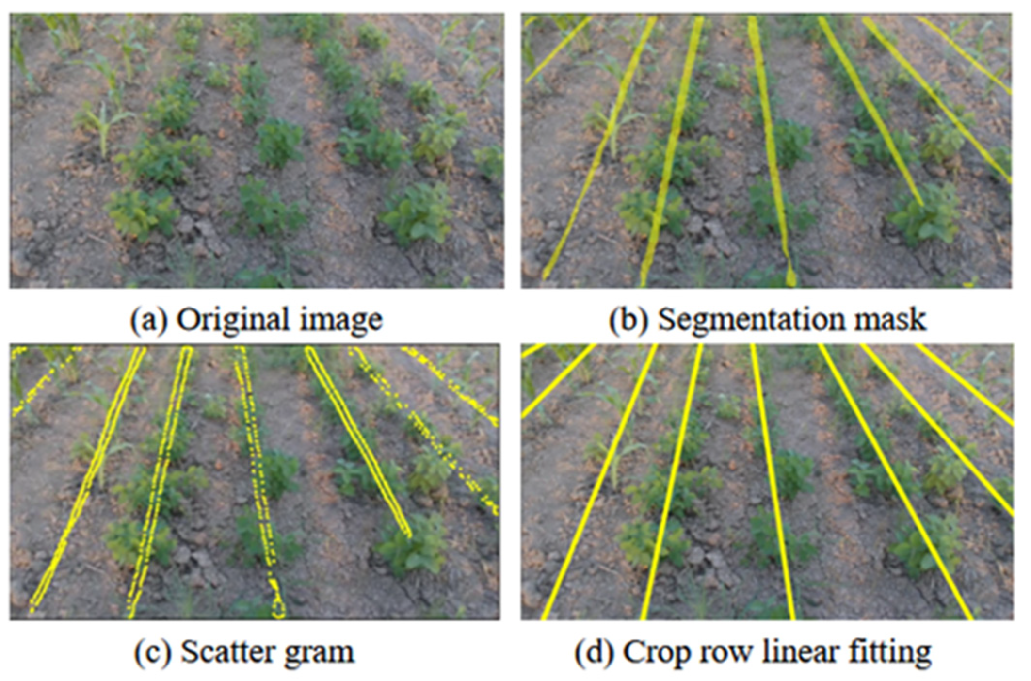
2.3.1. Crop Row Line Fitting

After completing the instance segmentation of crop rows and generating masks through GD-YOLOv10n-seg, the recognition results of each crop row were in the form of scattered points, as shown in Figure 10, which needed to be transformed morphologically to form the crop row lines. Through observation, it was found that the scatter masks of the crop rows were distributed in the shape of long strips and already had basic linear morphological characteristics (the predicted masks were shown as the yellow masks in Figure 10b. In order to quickly and effectively extract the crop row lines, principal component analysis (PCA) was used to fit a straight line through each mask based on its dominant orientation. The basic idea of PCA is to identify the main direction of the distribution of data points (the yellow points in Figure 10c and then find a straight line that minimizes the sum of the squares of the perpendicular distances from all data points to this line(the yellow lines in Figure 10d. The specific steps are as follows:

(1)

Data pre-processing: centering the mask data of all crop row scattergrams and subtracting each coordinate point from the average value of all points to ensure that the data are centered at the origin;

(2)

Construct covariance matrix: after calculating the covariance matrix of the centered data, this matrix reflects the magnitude of variance in each direction;

(3)

Solve for eigenvalues and eigenvectors: calculating the eigenvalues of the covariance matrix and the corresponding eigenvectors, which point out the main direction of the data distribution;

(4)

Extract the principal component straight line: Choosing the eigenvector corresponding to the largest eigenvalue as the direction of the fitted straight line. The straight line leading to this direction through the data center point is the required fitted straight line;

(5)

Calculate and plot the result: according to the direction of the obtained fitted straight line and the original center point, plot the straight line and calculate the projection of each scatter point to the straight line so as to verify the fitting effect of the straight line.

The advantage of the PCA is that it is very sensitive to the main trends in the data, and it is especially suitable for cases where the scatters have been arranged in a roughly straight line. This method is not only computationally efficient but also very suitable for occasions where the number of points is large or where there is a high demand for real-time performance, allowing rapid processing of large amounts of image data to identify crop rows. In addition, PCA shows strong robustness in processing noise-containing data and can effectively resist the influence of outliers. As the mask scatters have a basic straight line form, it is a reasonable and effective choice to use PCA for straight line fitting.

2.3.2. Test of Crop Row Line Extraction Effect

Under the soybean–corn compound planting mode, soybean and corn are planted by the same planting equipment at the same time and so the crop rows are parallel to each other. In the camera view, these crop rows converge to the top center of the image attachment position due to the principle of perspective [38]. Generally, the central part of the crop rows has obvious row spacing, while maintaining a high definition, and the spacing of the edge part is small as the adjacent crop rows are easily disturbed, which leads to false detection and missed detection in the recognition process. Therefore, after completing the acquisition of crop rows, it is necessary to select suitable crop rows for the generation of navigation lines. On the camera screen, which generally contains multiple crop rows, it is not necessary to use all the crop rows in the actual navigation lines generation [13,46], so the four crop rows in the center of the image are selected as the target crop rows. In order to judge the accuracy of the target row line extraction, the center line of the crop rows generated based on the labels is used as the reference row line, and the angle between the row line extracted based on the labels and the row line extracted by the algorithm in this paper is defined as the error angle for evaluating the accuracy of the target row line. When the error angle is greater than 5° [46], the crop row line extraction is considered invalid. Other evaluation metrics include the fitting time of the crop row center line.

The hardware and software environments for model training and testing are shown in

Table 1. Test platform.

Configuration	Parameter
Operation System	Windows 10 Professional Workstation Edition
CPU	Intel i5 13600KF (Intel, Santa Clara, CA, USA)
GPU	NVIDIA GTX4070ti 12GB (Nvidia, Santa Clara, CA, USA)
Acceletate Environment	Window 10 Profession
Python	3.8
Pytorch	2.0.1
Cuda	11.8
Cudnn	8.9.1
Data Annotation Tools	Labelme

.

3. Results

3.1. Performance of Segmentation Model

3.1.1. Performance of YOLOv10n-Seg Model

After dividing the dataset, the YOLOv10n-seg model was used as the baseline for training. The momentum factor was set to 0.937, with an initial learning rate of 0.01 and a batch size of 16. To prevent overfitting, an early stopping strategy was employed with a patience value of 100. The model was trained for up to 600 epochs, and the results are summarized in

Table 2. Performance comparison of YOLOv10n-seg and its improved versions.

Model	MPA /%	MIoU /%	MRecall /%	Speed /FPS	GFlops	Parameters /Million	Model Size /mb	Remarks
YOLOv10n -seg	58.18	42.04	59.00	149.54	11.7	2.84	5.75	Baseline
G-YOLO-v10n -seg	58.71	41.11	56.82	147.45	9.7	2.21	4.58	+GhostModule
GD-YOLO-v10n -seg	60.76	43.04	58.63	120.19	9.6	2.28	4.70	+GhostModule +DynamicConv

.

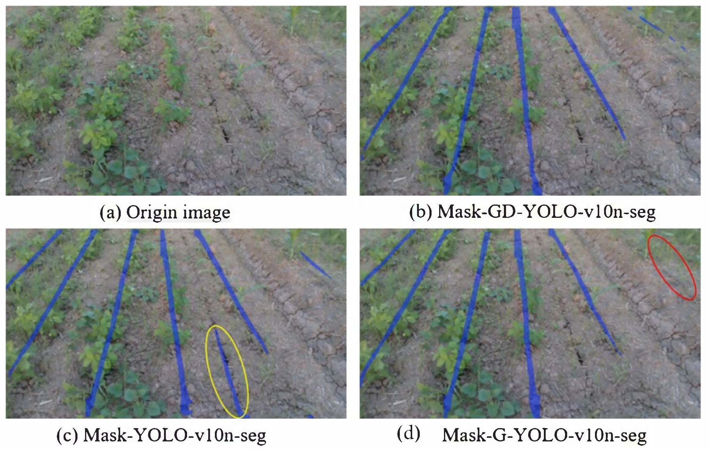
3.1.2. Performance of the Improved Model Based on GhostModule

To verify the impact of GhostModule on the detection performance of this model, this study trained with the improved model (G-YOLOv10n-seg) while ensuring that the hyperparameters, the number of iterations, and the training method remained unchanged during training.

After improving the original YOLOv10n-seg model with the GhostModule, the new model obtained a significant reduction in GFlops and the number of parameters, while the size of the model was reduced from the original 5.75 mb to 4.58 mb. Due to the lightweight nature of GhostModule, it achieved an improved computational efficiency by reducing the redundant convolutional operations, which in turn reduced the size of the model.

In terms of accuracy metrics, G-YOLOv10n-seg remained consistent with the baseline in terms of the MPA, but its decrease in MIoU implied that the model’s ability to differentiate between the boundaries of the crop rows is reduced. Specifically, MIoU measured the overlap between predicted and actual areas, and the decrease in MIoU suggested that the model may be more unclear in identifying the target area and so the match between predicted and actual areas has been weakened. Therefore, although the MPA remained basically unchanged, it may not be as accurate as the original YOLOv10-seg in terms of the precise location of areas and the definition of boundaries. The introduction of GhostModule significantly reduced the complexity and size of the model, but this came at a cost in that the model’s ability to capture detail was weakened for specific detection tasks, resulting in a small performance degradation. This drop in accuracy may stem from the fact that GhostModule reduced the redundant information in a portion of the feature maps in order to reduce the amount of computation and number of parameters, making the model exhibit slight instability in some complex scenes. This is especially true in scenes with more complex or detailed targets as the model may fail to adequately capture critical detail information, which in turn affects the MIoU. At the same time, the MRecall also showed a significant decrease, which meant that the model missed a portion of the real target when detecting and recognizing the target area. This further suggested that although G-YOLOv10n-seg was optimized in terms of model complexity and size, it did not perform as well as the original YOLOv10n-seg model in terms of the complete capture and accurate identification of target regions.

3.1.3. Performance of the Improved Model Based on DynamicConv-GhostModule

In order to further improve the model representation ability and reduce the accuracy degradation, DynamicConv was introduced on the basis of G-YOLOv10n-seg to form an improved version of the model based on DynamicConv-GhostModule (GD-YOLOv10n-seg). The introduction of DynamicConv enabled the convolution kernel to dynamically adjust the weights according to the input data, which enhanced the non-linear representation of the model and made up for the shortcomings of GhostModule in capturing complex features. With this improvement, the model could better adapt to the feature changes in the input image, which was expected to further improve the detection accuracy while keeping the model lightweight.

To verify the effectiveness of this improvement scheme, this study trained and tested the GD-YOLOv10n-seg model under the same dataset and hyperparameter conditions.

When DynamicConv was introduced, the GD-YOLOv10n-seg model further improved its accuracy while still being lightweight. The MIoU improved 1.93% compared to G-YOLO-v10n-seg and 1.00% compared to baseline. The MPA improved 2.05% compared to G-YOLO-v10n-seg and 2.58% compared to baseline.

The slight decrease in processing speed (from 149.54 FPS to 120.19 FPS) in GD-YOLOv10n-seg compared to the baseline YOLOv10n-seg was primarily due to the following:

(1)

DynamicConv operations: the introduced dynamic convolution adapted kernel weights per input, adding minor computational overhead.

(2)

Enhanced feature representation: while GhostModule reduced parameters, DynamicConv increased the model adaptability, trading off some speed for improved accuracy.

Despite the decrease in speed (FPS), its GFlops and model size were still significantly lower than the baseline. The introduction of DynamicConv effectively enhanced the model’s ability to capture the target area and boundary fineness and made up for the previous shortcomings of G-YOLOv10n-seg in precise positioning and detail capturing, which ultimately led to the optimization of the overall detection performance. In summary, GhostModule significantly reduced the complexity of the model, making it more suitable for resource-constrained scenarios such as mobile devices, and by introducing DynamicConv, GD-YOLOv10n-seg improved the overall accuracy of the model while keeping it lightweight.

As shown in Figure 11, the qualitative comparison of segmentation masks demonstrated the improvements achieved by GD-YOLOv10n-seg: GD-YOLOv10n-seg (Figure 11b) maintained complete detection of both central and edge crop rows, with accurate mask continuity. This validated the combined benefits of GhostModule’s efficiency and DynamicConv’s adaptive feature extraction. Baseline YOLOv10n-seg (Figure 11c) exhibited false positives, notably misidentifying field furrows as crop rows (yellow circle in Figure 11c), which would lead to navigation errors in practice. G-YOLOv10n-seg (Figure 11d) showed partial failures at field edges (red circle in Figure 11d), confirming that GhostModule alone could not address complex edge features. The comparison underscores that DynamicConv’s kernel adaptation was essential for distinguishing crops from similar-looking soil features.

3.1.4. Comparison with Other Segmentation Algorithms

The GD-YOLOv10n-seg model was compared with other commonly used instance segmentation models, including YOLOv5n-seg, YOLOv6n-seg, YOLOv8n-seg, YOLOv9t-seg, YOLOv11n-seg, and YOLOv12n-seg. The input parameters were strictly controlled, including uniform input size, the same dataset, and the training parameters. In addition to the instance segmentation, semantic segmentation algorithms are also often used in crop row generation and so U-Net algorithm [47] and DeepLabv3+ [48] algorithms were tested as comparison models. The comparison results are shown in

Table 3. Recognition performance of different models.

Model	MPA/%	MIoU/%	MRecall/%	Speed/FPS	Model Size/mb
GD-YOLO-v10n-seg	60.76	43.04	58.63	120.19	4.70
YOLOv10n-seg	58.18	42.04	59.00	149.54	5.75
YOLOv12n-seg	56.71	41.29	59.11	110.43	5.81
YOLOv11n-seg	57.98	41.55	58.41	134.05	5.76
YOLOv9t-seg	57.15	41.75	59.34	103.67	6.61
YOLOv8n-seg	56.50	41.50	59.52	158.42	6.48
YOLOv6n-seg	55.26	40.43	58.87	172.83	8.65
YOLOv5n-seg	57.35	41.32	58.35	164.41	5.55
U-Net	54.49	37.39	52.81	8.58	94.9
DeepLabv3+	53.65	40.31	60.42	7.91	22.4

.

By comparing the data in Table 3, it can be seen that the improved GD-YOLO-v10n-seg model demonstrated superior performance in the crop row detection task, especially in the MPA and MIoU, which were higher than those of the other models. Although DeepLabv3+ was slightly ahead in MRecall, its processing speed was only 7.91 FPS, which was significantly lower than the YOLO-series models, limiting its applicability in real-time application scenarios.

Among the instance segmentation algorithms of the YOLO series, GD-YOLO-v 10 n-seg not only performed well in recognition accuracy but also had a model size of only 4.70 mb, which made it the smallest among all the compared models. This means that GD-YOLO-v10n-seg can be deployed more flexibly in resource-constrained environments while maintaining efficient performance. In addition, GD-YOLO-v10n-seg suffered less loss in processing speed at 120.19 FPS, which ensured a fast response in applications.

In summary, the balance between high recognition accuracy, small model size, and good processing speed of the GD-YOLO-v10n-seg model made it particularly suitable for the crop row detection tasks. This characteristic made the GD-YOLO-v10n-seg an ideal choice in scenarios where fast and accurate image analysis is required.

3.2. Crop Row Line Fitting Results

When applying deep learning algorithms for crop row detection, we observed that detection performance was noticeably poorer at the edges of the camera view compared to the center. This discrepancy is primarily attributed to the uneven distribution of crop rows in the training data; rows in the central region appeared more frequently, allowing the model to learn their features more effectively. In contrast, fewer samples from the edge regions resulted in limited feature learning, thereby reducing detection accuracy in those areas. We chose the four crop rows in the center of the image to be the target rows. We used the ordinary least squares (OLSs) [35] and the random sample consistency algorithm (RANSAC) [49] to fit the crop row lines and compare them with the PCA. The evaluation metrics were line fitting speed v (FPS), crop row line angular deviation θ, and crop row line recognition accuracy P. Here, the fitting speed included the process of recognition processing of the original input image using GD-YOLO-v10n-seg, which was calculated as shown in Equation (9):

$$\begin{array}{c}\begin{array}{c}\begin{array}{cc}t={\displaystyle \frac{1}{N}}{\displaystyle \sum _{i=1}^N}{t}_i& v={\displaystyle \frac{1000}{t}}\end{array}\\ \theta ={\displaystyle \frac{1}{N}}{\displaystyle \sum _{i=1}^N}\left({\displaystyle \frac{1}{q}}{\displaystyle \sum _{j=1}^q}arctan\left|{\displaystyle \frac{k_{1j}-k_{2j}}{1+k_{1j}{k}_{2j}}}\right|\right)\end{array}\end{array}$$

(9)

where j is the jth line in the crop row image, q is the total number of lines in the image, N is the number of images in the test set, t_i is the line fitting time of the ith image (ms), k_1j is the slope of the true line of the jth crop row in the image (labeled crop row lines), and k_2j is the slope of the algorithmically fitted line of the jth crop row in the image. When the angle between the true line and the corresponding fitted line is less than 5°, it indicates that the crop row line fitting is valid, and the line recognition accuracy P is the ratio of the number of fitted valid lines to the number of actual crop rows. The results of crop row line detection for different algorithms are shown in

Table 4. Crop row line evaluation indicators.

Algorithms	Accuracy/%	Line Angular Deviation/°	Speed/FPS
PCA	95.08	1.75	61.47
OLSs	94.67	1.88	61.31
RANSAC	93.83	1.99	34.65

.

Compared with the RANSAC and the OLSs algorithm, the PCA algorithm showed a higher detection accuracy of 95.08% in the crop row line detection results, as well as a relatively low average crop row angular deviation (1.75°), which suggested that the PCA algorithm was able to better maintain the angular consistency of the crop row lines while ensuring the detection accuracy. Although PCA was slightly slower than the OLSs algorithm in terms of overall processing speed, its advantages in detection accuracy and angular deviation made PCA a better choice. Combined with these indicators, the PCA algorithm not only provides more accurate detection results but also ensures the processing speed and efficiency, which makes it suitable for application in agricultural operations.

4. Discussion

In this study, we proposed a crop row detection and line fitting method based on the improved YOLOv10n-seg algorithm for autonomous agricultural robots operating in the soybean and corn compound planting mode. Firstly, we chose the YOLOv10n-seg as the baseline and used DynamicConv and GhostModule to reduce the size and improve the baseline. The size of the improved GD-YOLO-v10n-seg was reduced by 1.05 mb compared to the baseline, and at the same time, the MPA and MIoU are improved by 2.48% and 0.86%, respectively. Unlike the currently used semantic segmentation algorithms [50,51] and target detection algorithms [36,52], GD-YOLO-v10n-seg, as an instance segmentation algorithm, was able to differentiate each crop row mask while segmenting the crop rows without the need for post-processing for target crop row extraction. This operation enabled the GD-YOLO-v10n-seg to significantly improve the speed of crop row detection (

Table 5. Crop row detection and processing speed under different algorithms.

Algorithm	Target Crop	Speed/FPS	Reference
GD-YOLOv10n-seg	soybean, corn	61.47 (total)	ours
U-Net-based	potato	1.9 (total)	[50]
E-Net-based	sugar beet	17 (recognition)	[51]
YOLOX-based	corn	23.8 (total)	[36]
YOLO-based	paddy	≤25 (total)	[52]
RGB-based	paddy	5 (total)	[53]

), which was of great importance for field navigation with high real-time requirements.

On the other hand, dataset construction and label processing remain critical components of deep learning-based crop row detection as they directly influence the overall model accuracy and the precision of crop row line extraction [50]. In the task of the label processing, the conventional semantic segmentation algorithms need to stroke the crop rows [50,51] which undoubtedly increases the workload of data preparation, especially in the face of a large number of datasets, and so the line labeling form is used in the preparation of dataset labeling in this study. This operation only requires delineation according to the distribution of the crop rows, which is less difficult and less workload than the conventional process. Although the mask accuracy was lower than the semantic segmentation algorithms [50], it also achieved a high level of accuracy and low angular error in the actual crop row detection (95.08% accuracy and 1.75° angular deviation). This result demonstrates the feasibility of using line labels for crop row labeling, which is consistent with the findings of Silva et al. (2023) [47]. The use of line labels was particularly effective when dealing with large-scale datasets. The method will be further improved at a later stage, such as adjusting the line width and adding the folding operation according to the direction of the crop rows, etc.

5. Limitations and Future Work

While the integration of the GD-YOLOv10n-seg model with PCA-based crop row line fitting demonstrates promising performance, several inherent limitations warrant further investigation. The performance of the model is highly dependent on the quality and diversity of the training dataset. The training dataset may not fully capture all real-world field conditions, such as extreme weather, dense weeds, or irregular planting patterns. Additionally, although the line annotation method is effective, it may lead to inaccuracies in complex situations, such as overlapping crop rows or severe occlusions. The current system is optimized for soybean–corn intercropping, and its applicability to other crop types or intercropping systems remains untested. Moreover, while the model achieves a high processing speed, real-time performance may be constrained by hardware limitations, especially in resource-limited environments. The current PCA-based approach excels in straight-row detection but shares a common limitation with most linear fitting methods [35,46,47,50]: it assumes crop rows follow a straight-line geometry. While this holds for most soybean–corn intercropping systems (Figure 2), highly curved or discontinuous rows may require alternative methods. Future studies could explore applying PCA to localized row segments and then connecting them with a non-linear curve. The system’s sole reliance on visual data limits its robustness under challenging conditions such as low visibility.

Future work will focus on expanding the dataset to include more diverse conditions, developing advanced fitting methods for irregular crop rows, and integrating other sensing technologies such as lidar to improve accuracy and robustness. Energy-efficiency optimization and field trials in different geographical regions will also be prioritized to enhance the versatility and practicality of the system in real-world agricultural applications. Meanwhile, we recognize the importance of expanding operational capabilities to more demanding conditions. Our future research will explore adaptation to low-light and night-time scenarios through enhanced data collection and system optimization. Additionally, the reported processing speeds (61.47 FPS) reflect high-performance GPU conditions. Actual edge-device performance may vary based on hardware specifications. Future work will include standardized benchmarking on agricultural computing platforms like NVIDIA Jetson AGX Orin (Nvidia, Santa Clara, CA, USA).

6. Conclusions

This study aimed to develop an intelligent detection method for crop rows in the soybean–corn compound planting mode. We proposed a real-time soybean–corn crop row detection method based on GD-YOLOv10n-seg with PCA fitting for autonomous agricultural robots operating in the soybean and corn compound planting mode. The experimental results show that after improving the original YOLOv10n-seg using GhostModule and DynamicConv, the GD-YOLO-v10n-seg model obtains a significant reduction in GFlops and the model size whilst at the same time outperforming other segmentation models in terms of MPA and MIoU. The improved model strikes a good balance between recognition effectiveness and model size, while the high processing speed makes it suitable for real-time applications in agricultural scenarios. In addition, the use of PCA for crop row line fitting is appropriate due to its excellent detection accuracy and processing speed.

These results confirm that the proposed method effectively addresses the challenges of semi-structured field environments and provides a reliable navigation reference for the automated agricultural machinery.

References

1. Wang, X.T.; Xi, X.B.; Chen, M.; Huang, S.J.; Jin, Y.F.; Zhang, R.H. Development Status of Soybean-Corn Strip Intercropping Technology and Equipment. Jiangsu Agric. Sci. 2023, 51, 36–45, (In Chinese with English Abstract). [Google Scholar]
2. Gerrish, J.B.; Stockman, G.C.; Mann, L.; Hu, G. Path-finding by image processing in agricultural field operations. SAE Trans. 1986, 95, 540–554. [Google Scholar]
3. Li, D.; Li, B.; Long, S.; Feng, H.; Wang, Y.; Wang, J. Robust detection of headland boundary in paddy fields from continuous RGB-D images using hybrid deep neural networks. Comput. Electron. Agric. 2023, 207, 107713. [Google Scholar]
4. Rabab, S.; Badenhorst, P.; Chen, Y.P.P.; Daetwyler, H.D. A template-free machine vision-based crop row detection algorithm. Precis. Agric. 2021, 22, 124–153. [Google Scholar]
5. Mousazadeh, H. A technical review on navigation systems of agricultural autonomous off-road vehicles. J. Terra Mech. 2013, 50, 211–232. [Google Scholar]
6. Winterhalter, W.; Fleckenstein, F.; Dornhege, C.; Burgard, W. Localization for precision navigation in agricultural fields—Beyond crop row following. J. Field Robot. 2021, 38, 429–451. [Google Scholar]
7. Gao, G.; Xiao, K.; Jia, Y. A spraying path planning algorithm based on colourdepth fusion segmentation in peach orchards. Comput. Electron. Agric. 2020, 173, 105412. [Google Scholar]
8. Rivera, G.; Porras, R.; Florencia, R.; Sánchez-Solís, J.P. LiDAR applications in precision agriculture for cultivating crops: A review of recent advances. Comput. Electron. Agric. 2023, 207, 107737. [Google Scholar]
9. Zhang, S.; Ma, Q.; Cheng, S.; An, D.; Yang, Z.; Ma, B.; Yang, Y. Crop Row Detection in the Middle and Late Periods of Maize under Sheltering Based on Solid State LiDAR. Agriculture 2022, 12, 2011. [Google Scholar] [CrossRef]
10. Tsiakas, K.; Papadimitriou, A.; Pechlivani, E.M.; Giakoumis, D.; Frangakis, N.; Gasteratos, A.; Tzovaras, D. An Autonomous Navigation Framework for Holonomic Mobile Robots in Confined Agricultural Environments. Robotics 2023, 12, 146. [Google Scholar] [CrossRef]
11. Farhan, S.M.; Yin, J.; Chen, Z.; Memon, M.S. A Comprehensive Review of LiDAR Applications in Crop Management for Precision Agriculture. Sensors 2024, 24, 5409. [Google Scholar] [CrossRef] [PubMed]
12. Wang, T.; Chen, B.; Zhang, Z.; Li, H.; Zhang, M. Applications of machine vision in agricultural robot navigation: A review. Comput. Electron. Agric. 2022, 198, 107085. [Google Scholar]
13. Li, X.; Su, J.H.; Yue, Z.C.; Wang, S.C.; Zhou, H.B. Extracting navigation line to detect the maize seedling line using median-point Hough transform. Trans. Chin. Soc. Agric. Eng. 2022, 38, 167–174, (In Chinese with English Abstract). [Google Scholar]
14. Bawden, O.; Kulk, J.; Russell, R.; McCool, C.; English, A.; Dayoub, F.; Lehnert, C.F.; Perez, T. Robot for weed species plant-specific management. J. Field Robot. 2017, 34, 1179–1199. [Google Scholar]
15. Lan, T.; Li, R.L.; Zhang, Z.H.; Yu, J.G.; Jin, X.J. Analysis on research status and trend of intelligent agricultural weeding robot. Comput. Meas. Control. 2021, 29, 1–7, (In Chinese with English Abstract). [Google Scholar]
16. Zhang, W.; Miao, Z.; Li, N.; He, C.; Sun, T. Review of Current Robotic Approaches for Precision Weed Management. Curr. Robot. Rep. 2022, 3, 139–151. [Google Scholar]
17. Jørgensen, R.N.; Sørensen, C.A.; Pedersen, J.M.; Havn, I.; Jensen, K.; Søgaard, H.T.; Sørensen, L.B. HortiBot: A System Design of a Robotic Tool Carrier for High-tech Plant Nursing. Agric. Eng. Int. CIGR J. 2007, 9, 14075959. [Google Scholar]
18. Bai, Y.H.; Zhang, B.H.; Xu, N.M.; Zhou, J.; Shi, J.Y.; Diao, Z.H. Vision-based navigation and guidance for agricultural autonomous vehicles and robots: A review. Comput. Electron. Agric. 2023, 205, 107584. [Google Scholar]
19. Zhou, Y.; Yang, Y.; Zhang, B.L.; Wen, X.; Yue, X.; Chen, L. Autonomous detection of crop rows based on adaptive multi-ROI in maize fields. Int. J. Agric. Biol. Eng. 2021, 14, 1934–6344. [Google Scholar]
20. Søgaard, H.T.; Olsen, H.J. Determination of crop rows by image analysis without segmentation. Comput. Electron. Agric. 2003, 38, 141–158. [Google Scholar]
21. Li, M.; Zhang, M.; Meng, Q. Rapid detection method of agricultural machinery visual navigation baseline based on scanning filtering. Trans. Chin. Soc. Agric. Eng. 2013, 29, 41–47, (In Chinese with English Abstract). [Google Scholar]
22. Montalvo, M.; Pajares, G.; Guerrero, J.M.; Romeo, J.; Guijarro, M.; Ribeiro, A.; Ruz, J.J.; Cruz, J.M. Automatic detection of crop rows in maize fields with high weeds pressure. Expert Syst. Appl. 2012, 39, 11889–11897. [Google Scholar]
23. Yu, Y.; Bao, Y.; Wang, J.; Chu, H.; Zhao, N.; He, Y.; Liu, Y. Crop Row Segmentation and Detection in Paddy Fields Based on Treble-Classification Otsu and Double-Dimensional Clustering Method. Remote Sens. 2021, 13, 901. [Google Scholar] [CrossRef]
24. Leemans, V.; Destain, M.F. Line cluster detection using a variant of the Hough transform for culture row localisation. Image Vis. Comput. 2006, 24, 541–550. [Google Scholar]
25. Yang, X.; Li, X. Research on Autonomous Driving Technology Based on Deep Reinforcement Learning. Netw. Secur. Technol. Appl. 2021, 1, 136–138. [Google Scholar]
26. Hwang, J.H.; Seo, J.W.; Kim, J.H.; Park, S.; Kim, Y.J.; Kim, K.G. Comparison between Deep Learning and Conventional Machine Learning in Classifying Iliofemoral Deep Venous Thrombosis upon CT Venography. Diagnostics 2022, 12, 274. [Google Scholar] [CrossRef]
27. Niu, S.; Liu, Y.; Wang, J.; Song, H. A Decade Survey of Transfer Learning (2010–2020). Trans. Artif. Intell. 2020, 1, 151–166. [Google Scholar]
28. Zhao, C.; Wen, C.; Lin, S.; Guo, W.; Long, J. A method for identifying and detecting tomato flowering period based on cascaded convolutional neural network. Trans. Chin. Soc. Agric. Eng. 2020, 36, 143–152, (In Chinese with English Abstract). [Google Scholar]
29. Hu, R.; Su, W.H.; Li, J.L.; Peng, Y.K. Real-time lettuce-weed localization and weed severity classification based on lightweight YOLO convolutional neural networks for intelligent intra-row weed control. Comput. Electron. Agric. 2024, 226, 109404. [Google Scholar]
30. Wen, C.J.; Chen, H.R.; Ma, Z.Y.; Zhang, T.; Yang, C.; Su, H.Q.; Chen, H.B. Pest-YOLO: A model for large-scale multi-class dense and tiny pest detection and counting. Front. Plant Sci. 2022, 13, 973985. [Google Scholar]
31. Li, J.; Yin, J.; Deng, L. A robot vision navigation method using deep learning in edge computing environment. EURASIP J. Adv. Signal Process. 2021, 22, 1–20. [Google Scholar]
32. Adhikari, S.P.; Kim, G.; Kim, H. Deep Neural Network-based System for Autonomous Navigation in Paddy Field. IEEE Access 2020, 8, 71272–71278. [Google Scholar]
33. Ponnambalam, V.R.; Bakken, M.; Moore, R.J.D.; Gjevestad, J.G.O.; From, P.J. Autonomous Crop Row Guidance Using Adaptive Multi-ROI in Strawberry Fields. Sensors 2020, 20, 5249. [Google Scholar] [CrossRef] [PubMed]
34. Bah, M.; Hafiane, A.; Canals, R. CRowNet: Deep Network for Crop Row Detection in UAV Images. IEEE Access 2020, 8, 5189–5200. [Google Scholar]
35. Ruan, Z.; Chang, P.; Cui, S.; Luo, J.; Gao, R.; Su, Z. A precise crop row detection algorithm in complex farmland for unmanned agricultural machines. Biosyst. Eng. 2023, 232, 1–12. [Google Scholar]
36. Gong, H.; Zhuang, W.; Wang, X. Improving the maize crop row navigation line recognition method of YOLOX. Front. Plant Sci. 2024, 15, 1338228. [Google Scholar]
37. Liu, H.; Xiong, W.; Zhang, Y. YOLO-CORE: Contour Regression for Efficient Instance Segmentation. Mach. Intell. Res. 2023, 20, 716–728. [Google Scholar]
38. Wang, A.; Chen, H.; Liu, L.H.; Chen, K.; Lin, Z.J.; Han, J.G.; Ding, G.G. YOLOv10: Real-Time End-to-End Object Detection. Adv. Neural Inf. Process. Systems 2024, 37, 107984–108011. [Google Scholar]
39. Li, X.G.; Zhao, W.; Zhao, L.L. Extraction algorithm of the center line of maize row in case of plants lacking. Trans. Chin. Soc. Agric. Eng. 2021, 37, 203–210, (In Chinese with English Abstract). [Google Scholar]
40. Han, K.; Wang, Y.; Tian, Q.; Guo, J.; Xu, C.; Xu, C. Ghostnet: More features from cheap operations. In Proceedings of the IEEE/CVF Conference on Computer Vision and Pattern Recognition, Nashville, TN, USA, 13–19 June 2020; pp. 1580–1589. [Google Scholar]
41. Yan, H.W.; Wang, Y. UAV Object Detection Model Based on Improved Ghost Module. J. Phys. Conf. Ser. 2022, 2170, 012013. [Google Scholar]
42. Yang, L.; Cai, H.; Luo, X.; Wu, J.; Tang, R.; Chen, Y.; Li, W. A lightweight neural network for lung nodule detection based on improved ghost module. Quant. Imaging Med. Surg. 2023, 13, 4205–4221. [Google Scholar] [PubMed]
43. Chen, Y.; Li, J.; Sun, K.; Zhang, Y. A lightweight early forest fire and smoke detection method. J. Supercomput. 2024, 80, 9870–9893. [Google Scholar]
44. Han, K.; Wang, Y.H.; Guo, J.Y.; Wu, E.H. ParameterNet: Parameters Are All You Need for Large-scale Visual Pretraining of Mobile Networks. In Proceedings of the IEEE/CVF Conference on Computer Vision and Pattern Recognition, Seattle, WA, USA, 16–22 June 2024. [Google Scholar]
45. Chen, Y.; Dai, X.; Liu, M.; Chen, D.; Yuan, L.; Liu, Z. Dynamic Convolution: Attention Over Convolution Kernels. In Proceedings of the 2020 IEEE/CVF Conference on Computer Vision and Pattern Recognition (CVPR), Seattle, WA, USA, 13–19 June 2020; pp. 11027–11036. [Google Scholar]
46. Yang, Y.; Zhang, B.L.; Zha, J.Y.; Wen, X.; Chen, L.Q.; Zhang, T.; Dong, X.; Yang, X.J. Real-time extraction of navigation line between corn rows. Trans. Chin. Soc. Agric. Eng. 2020, 36, 162–171, (In Chinese with English Abstract). [Google Scholar]
47. Silva, R.D.; Cielniak, G.; Wang, G.; Gao, J. Deep learning-based crop row detection for infield navigation of agri-robots. J. Field Robot. 2022, 41, 2299–2321. [Google Scholar]
48. Lin, S.J.; Chen, Q.; Chen, J.J. Ridge-furrow Detection in Glycine Max Farm Using Deep Learning. In Proceedings of the 2020 International Conference on Pervasive Artificial Intelligence (ICPAI), Taipei, Taiwan, 3–5 December 2020; pp. 183–187. [Google Scholar]
49. Fu, D.B.; Chen, Z.Y.; Yao, Z.Q.; Liang, Z.P.; Cai, Y.H.; Liu, C.; Tang, Z.Y.; Lin, C.X.; Feng, X.; Qi, L. Vision-based trajectory generation and tracking algorithm for maneuvering of a paddy field robot. Comput. Electron. Agric. 2024, 226, 109368. [Google Scholar]
50. Yang, R.; Zhai, Y.; Zhang, J.; Zhang, H.; Tian, G.; Zhang, J.; Huang, P.; Li, L. Potato Visual Navigation Line Detection Based on Deep Learning and Feature Midpoint Adaptation. Agriculture 2022, 12, 1363. [Google Scholar] [CrossRef]
51. Cao, M.; Tang, F.; Ji, P.; Ma, F. Improved Real-Time Semantic Segmentation Network Model for Crop Vision Navigation Line Detection. Front. Plant Sci. 2022, 13, 898131. [Google Scholar]
52. Chen, X.J.; Wang, C.X.; Zhu, D.Q.; Liu, X.L.; Zou, Y.; Zhang, S.; Liao, J. Detection of rice seedling row lines based on YOLO convolutional neural network. Jiangsu J. Agric. Sci. 2020, 04, 930–935, (In Chinese with English Abstract). [Google Scholar]
53. Guo, X.Y.; Xue, X.Y. Extraction of navigation lines for rice seed field based on machine vision. J. Chin. Agric. Mech. 2021, 42, 197–201, (In Chinese with English Abstract). [Google Scholar]
Figure 1. Flow chart of the entire crop row center line extraction.
Agriculture 15 00796 g001
Figure 2. Crop row labeling (yellow lines represent the labeled crop row masks).
Agriculture 15 00796 g002
Figure 3. YOLOv10n-seg model (yellow masks represent the predicted crop row masks).
Agriculture 15 00796 g003
Figure 4. Label visualization of segmentation and object detection (yellow lines represent the labeled crop row masks and red boxes represent the corresponding object detection boxes).
Agriculture 15 00796 g004
Figure 5. The convolution layer and GhostModule: (a) the convolutional layer and (b) the GhostModule (Φk represents the cheap operation).
Agriculture 15 00796 g005
Figure 6. Illustration of C2f and C2f-GhosModule.
Agriculture 15 00796 g006
Figure 7. Illustration of DynamicConv (* stands for the multiply operation).
Agriculture 15 00796 g007
Figure 8. (GD-YOLOv10n-seg) network model (yellow masks represent the predicted crop row masks).
Agriculture 15 00796 g008
Figure 9. Intersection over union.
Agriculture 15 00796 g009
Figure 10. Crop row lines fitting.
Agriculture 15 00796 g010
Figure 11. Comparison of three algorithms for crop row mask detection (blue masks represent the predicted crop row masks).
Agriculture 15 00796 g011