Abstract
Daily reference crop evapotranspiration (ET0) is crucial for precision irrigation management, yet traditional prediction methods struggle to capture its dynamic variations due to the complexity and nonlinearity of meteorological conditions. To address this, we propose an Improved Informer model to enhance ET0 prediction accuracy, providing a scientific basis for agricultural water management. Using meteorological and soil data from the Yingde region, we employed the Maximal Information Coefficient (MIC) to identify key influencing factors and integrated Residual Cycle Forecasting (RCF), Star Aggregate Redistribute (STAR), and Fully Adaptive Normalization (FAN) techniques into the Informer model. MIC analysis identified total shortwave radiation, sunshine duration, maximum temperature at 2 m, soil temperature at 28–100 cm depth, and surface pressure as optimal features. Under the five-feature scenario (S3), the improved model achieved superior performance compared to Long Short-Term Memory (LSTM) and the original Informer models, with MAE reduced to 0.065 (LSTM: 0.637, Informer: 0.171) and MSE to 0.007 (LSTM: 0.678, Informer: 0.060). The inference time was also reduced by 31%, highlighting the enhanced computational efficiency. The Improved Informer model effectively captures the periodic and nonlinear characteristics of ET0, offering a novel solution for precision irrigation management with significant practical implications.
1. Introduction
As one of the world’s largest agricultural nations, China’s agricultural water consumption accounts for 62.2% of the national total water use, yet its agricultural water use efficiency is only 57.6% [1], significantly lower than advanced international levels. Conventional irrigation methods, which rely heavily on experience-driven flood irrigation, fail to account for the dynamic water needs of crops across different growth stages, leading to inefficient water use and a lack of scientific grounding [2].
Precision irrigation is essential for improving agricultural water use efficiency, with its core lying in the accurate estimation of crop water requirements [3]. Daily reference crop evapotranspiration (ET0) serves as a critical indicator for providing a scientific basis for irrigation decisions and optimizing water resource allocation [4]. The FAO-56 Penman–Monteith model, developed by the Food and Agriculture Organization of the United Nations (FAO), is widely used for ET0 calculation due to its high accuracy [5]. However, its dependence on multiple meteorological parameters and computational complexity limits its applicability in large-scale or resource-limited settings [6]. Furthermore, the nonlinear relationship between ET0 and meteorological factors poses challenges for traditional linear models, which struggle to capture its dynamic variations [7].
With the rapid development of machine learning and deep learning technologies, ET0 prediction methods based on artificial intelligence have gradually emerged. Researchers have constructed various prediction models, including traditional machine learning models and deep learning models [8]. Among them, deep learning models can be divided into traditional neural network models, models based on Recurrent Neural Networks (RNN), and models based on Transformer, each demonstrating different technical advantages and application potential [9].
Owing to their high computational efficiency and simple structure, traditional machine learning models were widely applied to ET0 prediction in the early stage. Kumar et al. used an Extreme Learning Machine (ELM) model to efficiently predict weekly ET0 in arid regions of India [10], while Talib et al. found that the Random Forest (RF) model outperformed the Long Short-Term Memory (LSTM) model in daily evapotranspiration prediction [11]. However, these models struggle with long-term dependencies, making them less suitable for high-precision irrigation [12].
In the field of deep learning, traditional neural network models (such as Artificial Neural Networks (ANNs) trained with the Back Propagation Neural Network (BP) algorithm) were among the first to be applied to ET0 prediction. Abdel-Fattah et al. evaluated regression models and ANNs for estimating ET0 in arid regions. They showed that ANNs achieved higher accuracy ( = 0.99), highlighting their potential for water management [13]. However, traditional neural network models have problems such as gradient disappearance and low computational efficiency when dealing with time series data, making it difficult to capture long-term dependencies.
To overcome the limitations of traditional neural networks, models based on RNN (such as LSTM and its variants) have become a research hotspot. Recurrent Neural Networks (RNNs) handle time series dependencies through their recurrent structure, but they suffer from gradient disappearance and explosion problems, limiting their performance in long-term sequence tasks [14]. LSTM networks effectively alleviate gradient disappearance through gating mechanisms (input gate, forget gate, and output gate), significantly enhancing their ability to capture long-term dependencies [15]. Liyew et al. compared various machine learning models for predicting actual evapotranspiration (AET) using meteorological data, demonstrating that deep learning models, particularly LSTM subjected to Bayesian optimization, outperformed classical methods like Support Vector Regression (SVR) and RF, achieving higher accuracy ( up to 0.8861) [16]. Gao et al. developed an enhanced MHSA-BiLSTM model for predicting reference evapotranspiration (ET0) by combining multi-head self-attention (MHSA) and bidirectional LSTM. The model incorporated historical ET0 features extracted using Seasonal-Trend Decomposition using Loess (STL). It achieved superior accuracy ( up to 0.9127) compared to traditional methods [17]. However, the recurrent structure of LSTM limits its parallel computing capabilities, resulting in low efficiency for long time series processing and a potential loss of key information in ultra-long sequences [18].
In recent years, models based on Transformer have brought new research directions to the field of ET0 prediction. Transformer abandons the recurrent structure of RNNs and uses multi-head self-attention mechanisms to simultaneously capture global dependencies in sequences, significantly enhancing its ability to model long-term dependencies [19]. Abed et al. introduced a novel Transformer Neural Network (TNN) to predict monthly pan evaporation in Malaysia. The TNN model achieved superior accuracy compared to LSTM and Convolutional Neural Network (CNN) models, with values reaching up to 0.989. Their work demonstrates the potential of TNN for evaporation forecasting and its applicability in water resource management [20]. However, Transformer models have high computational complexity and lack explicit modeling of local features, limiting their efficiency in practical applications.
To overcome the limitations of Transformer, researchers have proposed several improved models. Among them, the Informer model significantly reduces computational complexity through sparse attention mechanisms and distillation operations while enhancing its long-term sequence prediction performance [21]. Shang et al. used the Informer model for drought prediction and found that it significantly outperformed Autoregressive Integrated Moving Average (ARIMA) and LSTM models in long-term scales (e.g., the Standardized Precipitation Evapotranspiration Index at 24 months (SPEI24)) [22]. However, its application in ET0 prediction remains underexplored, with room for further optimization in feature selection and attention mechanisms.
In addition, feature selection techniques play a crucial role in improving model performance. Studies have shown that intelligent feature selection can significantly enhance prediction accuracy. Methods such as Maximal Information Coefficient (MIC) and Principal Component Analysis (PCA) have proven effective for feature screening and dimensionality reduction [23].
To address the above issues, this study proposes a daily reference crop evapotranspiration (ET0) prediction method based on an Improved Informer model. By combining the Maximal Information Coefficient (MIC) to screen key meteorological factors and introducing optimization techniques such as Residual Cycle Forecasting (RCF), Star Aggregate Redistribute (STAR), and Fully Adaptive Normalization (FAN) into the model, we aim to improve the accuracy and efficiency of ET0 prediction.
2. Materials and Methods
2.1. Study Area Description and Data Sources
The study area is located at the Tea Research Institute of Guangdong Academy of Agricultural Sciences (Yingde Experimental Base) in Yingde, Qingyuan City, Guangdong Province, covering an area of approximately 333,333 . Yingde is located in the north-central part of Guangdong, south of the mountainous terrain in northern Guangdong. It is situated at the confluence of three rivers and is predominantly characterized by its mountainous and hilly landscapes [24]. Figure 1 shows the location of Yingde. Yingde is situated in the transitional zone from the south subtropical to the middle subtropical climate, characterized by a subtropical monsoon climate with distinct seasons: the spring is rainy and cloudy, the summer is hot and humid, the autumn is cool and dry, and the winter is occasionally cold. The region has an average annual temperature of 21.1 °C, annual precipitation of 1906.2 mm, relative humidity of 77%, and annual sunshine duration of 1631.7 h. The warm and humid climate, with concurrent rainfall and heat, provides abundant water and heat resources and favorable light conditions for tea tree growth, contributing to the formation of high-quality floral and aromatic tea [25].
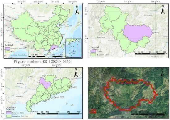
Figure 1.
The location of Yingde.
Details of the location in the dataset are summarized in Table 1. The dataset used in this study is derived from the fifth-generation European Centre for Medium-Range Weather Forecasts (ECMWF) climate reanalysis data (ERA5), covering meteorological records from Yingde from 2015 to 2024, comprising a total of 3562 data entries. The dataset includes the following variables: total shortwave radiation, 10 m wind direction and maximum wind speed at 10 m, sunshine duration, maximum and minimum temperatures at 2 m, average temperature at 2 m, relative humidity at 2 m, soil moisture and temperature at depths of 28–100 cm, surface pressure, and total precipitation. In harmony with the structure of the datasets, the 28–100 cm soil depth layer, as shown in the ERA5 reanalysis data of the soil moisture variables, is used (0–7 cm, 7–28 cm, 28–100 cm, and 100–289 cm). This depth aligns with the root distribution of most crops, as most crops typically have a root distribution within the depth range of 20–100 cm, including tea plants.

Table 1.
Details of the location in the dataset.
2.2. Data Preprocessing
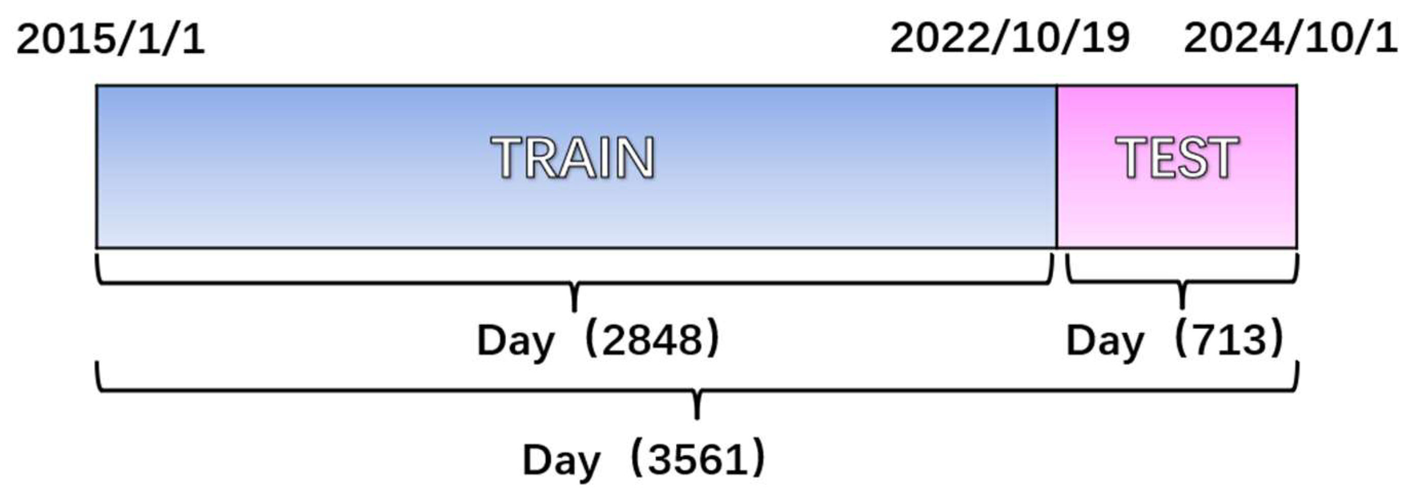
To ensure data quality, the dataset was subjected to rigorous preprocessing. First, outliers were detected and eliminated using the 3σ criterion [26], a statistically robust method for anomaly removal. This step primarily targets statistical anomalies that deviate significantly from expected climate patterns, rather than valid extreme weather events. The outlier proportion was low (0.28%), confirming the dataset’s overall reliability. Next, missing values were replaced through linear interpolation of temporally adjacent data points to preserve temporal continuity. The preprocessed dataset was then partitioned into training and testing subsets at an 8:2 ratio, containing 2849 and 713 samples, respectively. The data splitting methodology is visually summarized in Figure 2.

Figure 2.
Graphical train and test.
To address feature scale discrepancies, input variables were normalized to a [0, 1] range using min–max scaling, a widely adopted preprocessing method for stabilizing gradient-based optimization during model training [27]. The normalization formula is given by the following:
where is the original data point and and are the minimum and maximum values of the feature, respectively.
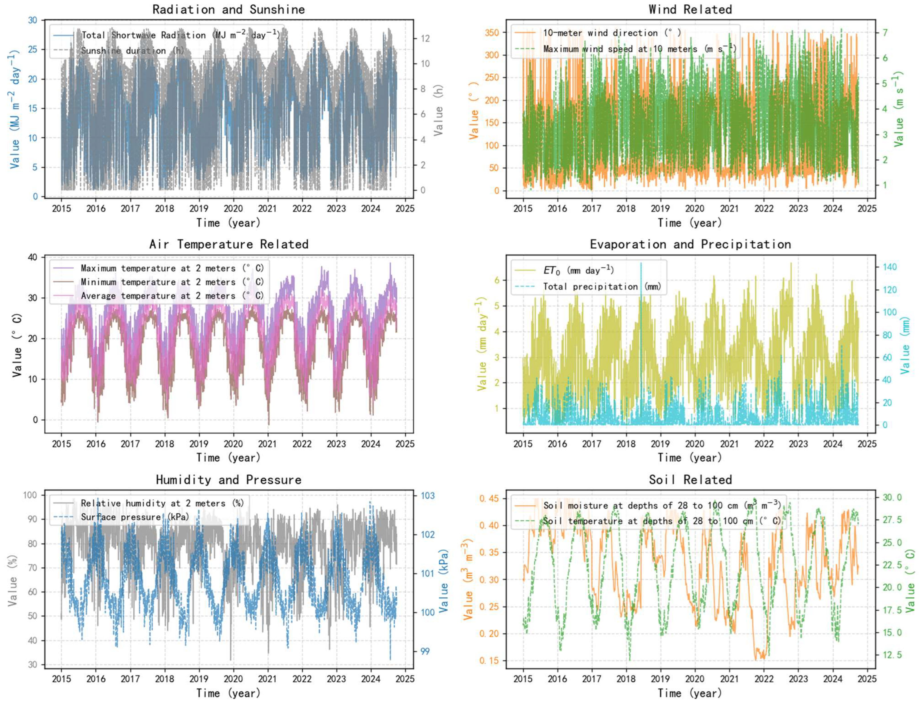
Figure 3 presents the statistical characteristics of reference crop evapotranspiration (ET0) and the corresponding variables within the dataset (1 January 2015–1 October 2024), highlighting distinct seasonal patterns and interannual variability. These fluctuations reflect regional climate dynamics and their potential environmental implications. Table 2 provides key descriptive metrics for the entire dataset, including the maximum, minimum, mean and standard deviation, serving as a foundation in time series modeling and evapotranspiration prediction.
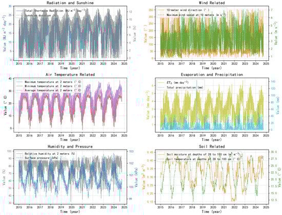
Figure 3.
ET0 and Corresponding Variables Analysis.
Table 2.
Descriptive Statistics of ET0 and Related Variables.
2.3. Calculation of Reference Crop Evapotranspiration (ET0)
Reference crop evapotranspiration (ET0) is a critical indicator for precision irrigation management and serves as the target variable in this study. ET0 was calculated using the FAO-56 Penman–Monteith model, which is widely recognized for its accuracy and applicability in various climatic conditions [28]. The formula for ET0 is given by Equation (2):
where is the reference crop evapotranspiration (mm ); is the net radiation at the crop surface (MJ ); is the soil heat flux density (MJ ); is the mean daily air temperature at 2 m height (°C); is the wind speed at 2 m height (m ); is the saturation vapor pressure (kPa); is the actual vapor pressure (kPa); Δ is the slope of the saturation vapor pressure curve (kPa ); and is the psychrometric constant (kPa ).
Since the FAO-56 Penman–Monteith equation requires wind speed at 2 m, we have converted the 10 m wind speed to the standard 2 m height using the following equation:
where is the wind speed at 10 m height (m ) and is the wind speed at 2 m height (m ).
2.4. Meteorological Scenarios
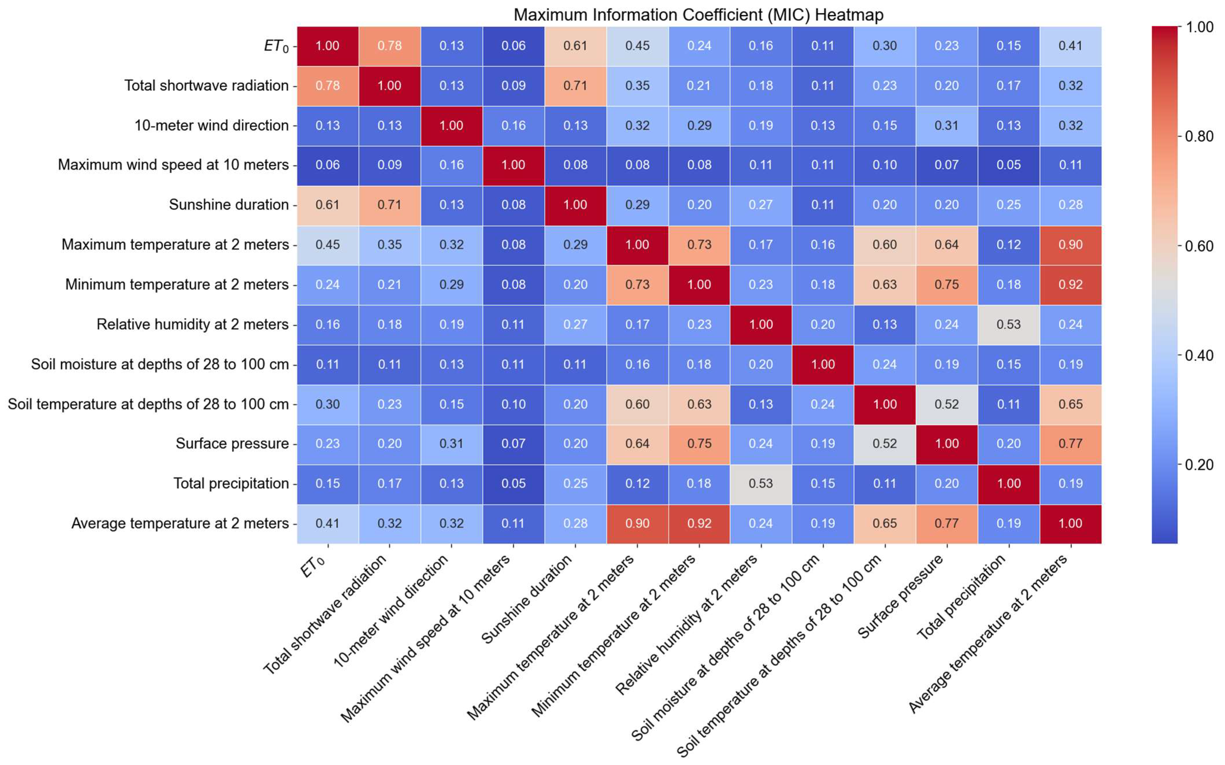
To address nonlinear dependencies between meteorological variables and reference crop evapotranspiration (ET0) while reducing computational complexity, this study employed the Maximal Information Coefficient (MIC) for feature selection. MIC is a statistical measure that quantifies mutual information between variables, capturing both linear and nonlinear relationships [29]. Unlike traditional linear methods such as the Pearson correlation coefficient, MIC adapts more effectively to complex interactions, making it ideal for identifying influential features in nonlinear systems.
Using Python 3.9’s MINE package, we calculated the Maximal Information Coefficient (MIC) between each meteorological variable and ET0. Higher MIC values indicated stronger influences on ET0, revealing the relative importance of each feature [30]. This process identified key meteorological factors affecting ET0, streamlining the subsequent analysis.
Figure 4 illustrates the MIC values between each feature variable and the reference crop evapotranspiration (ET0). Additionally, it indicates a high correlation among meteorological temperature variables, specifically the maximum temperature at 2 m, average temperature at 2 m, and minimum temperature at 2 m. This high correlation suggests significant redundancy among these temperature variables. To avoid redundancy and enhance the modeling efficiency and predictive performance, the maximum temperature at 2 m was selected as the representative meteorological temperature variable for subsequent modeling analysis. This selection aims to retain the most informative temperature-related feature while reducing redundancy.
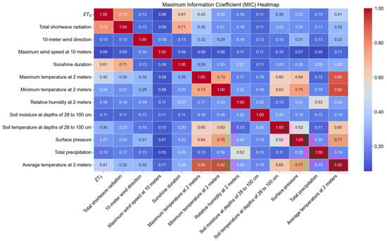
Figure 4.
The Maximum Information Coefficient Heatmap Between Feature Variables and ET0.
We ranked the features by their MIC values, reflecting their relative importance in predicting ET0. The top three features—total shortwave radiation (MIC: 0.78), sunshine duration (MIC: 0.61), and maximum temperature at 2 m (MIC: 0.45)—were identified as the most influential and selected for further analysis.
To evaluate their contributions to ET0 simulation, we designed multiple scenarios (Table 3). Scenario S1 includes only the top three features with the highest MIC values. In subsequent scenarios (S2–S8), additional features are progressively introduced one at a time, following a descending order of MIC values—that is, each new scenario incorporates the next feature with the highest remaining MIC value until the top 10 features are included. These scenarios enable systematic assessment of how different feature combinations affect model performance, ultimately determining the optimal feature set for ET0 prediction.
Table 3.
Details of Meteorological Scenarios.
2.5. Deep Learning Methods
The Informer, Improved Informer, and LSTM models were used in this paper.
2.5.1. Long Short-Term Memory
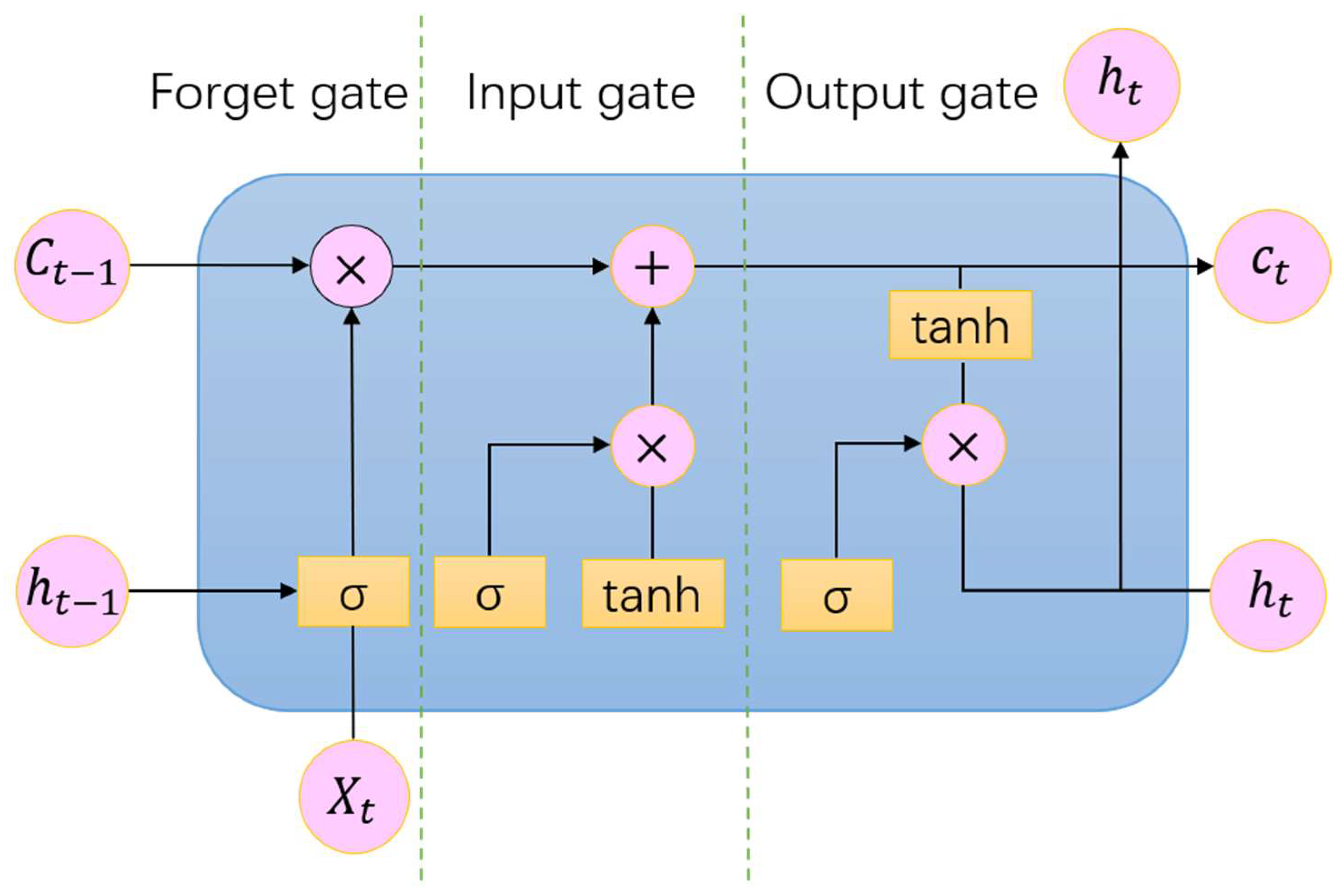
Long Short-Term Memory (LSTM), a specialized recurrent neural network (RNN), addresses the vanishing and exploding gradient issues common in traditional RNNs during long sequence training [31]. Through its gating mechanism—input, forget, and output gates—LSTM dynamically regulates information storage, updating, and retrieval, maintaining stable gradient propagation across prolonged sequences [32]. Central to this architecture is the cell state, which serves as a continuous pathway for retaining long-term dependencies. The LSTM cell operates through the following steps:
- Step 1: Compute the Forget Gate
The forget gate determines the extent to which past information from the previous cell state should be retained or discarded. It is computed as follows:
where is the forget gate output; and are the weight matrix and bias term for the forget gate, respectively; represents the hidden state from the previous time step; is the input at the current time step; and σ(⋅) denotes the sigmoid activation function.
- Step 2: Compute the Input Gate and Candidate Cell State
The input gate determines how much new information should be incorporated into the cell state, while the candidate cell state proposes new information to be added.
where regulates the proportion of new information; and are the weight matrix and bias term for the input gate, respectively; and is the candidate cell state, which is transformed via a tanh activation function to ensure values are in the range [−1, 1].
- Step 3: Update the Cell State
The cell state is updated by combining the retained past information (scaled by the forget gate) and the newly added information (scaled by the input gate).
where denotes element-wise multiplication (Hadamard product).
- Step 4: Compute the Output Gate and Hidden State
The output gate regulates how much of the updated cell state contributes to the hidden state , which serves as the final output at the current time step.
where is the output gate output and is the hidden state.
Figure 5 shows the structure of LSTM in detail. However, LSTM may still encounter difficulties when processing extremely long sequences, as it remains susceptible to gradient vanishing or exploding issues [33].
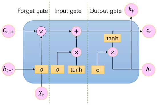
Figure 5.
LSTM model structure diagram.
2.5.2. Informer
Informer is a state-of-the-art deep learning model designed explicitly for long-sequence time-series forecasting tasks. It addresses the computational inefficiencies associated with the Transformer architecture, which typically suffers from quadratic complexity O() due to its self-attention mechanism, where L represents the sequence length.
Self-Attention Mechanism Improvement
The self-attention mechanism in the Transformer model is defined as follows:
where , and are the query, key, and value matrices, respectively, and d is the feature dimension.
Each query computes its attention weights based on all keys , resulting in the following:
Since every query attends to every key, the time complexity for computing self-attention is quadratic, namely, O(). This quadratic complexity is a major bottleneck when handling long sequences, as it leads to excessive memory consumption and computational overhead.
To overcome the inefficiency of full self-attention, Informer introduces Multi-Head ProbSparse Attention, which reduces the computational complexity from O() to O(). Instead of computing attention for all tokens, only the most informative queries are retained, based on an importance score.
where measures the information richness of query . The mechanism then selects the top u = clogL queries with the highest scores, filtering out redundant computations.
The final sparse attention formulation is as follows:
where contains only the top u queries. This optimization significantly reduces computation and memory usage while preserving long-range dependencies, making Informer well-suited for efficient long-sequence forecasting.
Figure 6 presents the Informer model, which introduces several key features to improve efficiency in long-sequence time-series forecasting, including the ProbSparse self-attention mechanism, sequence distillation, parallel generative decoding, masks and fully connected layers in the decoder. The following sections describe the role of these components in the Informer model, along with the data flow from input to output.
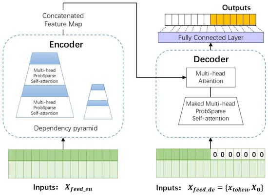
Figure 6.
Informer model structure diagram.
The encoder of the Informer model processes the input time-series sequence. Informer adopts the ProbSparse self-attention mechanism to address the limitations of standard self-attention. By employing a sparse sampling strategy that focuses on the most informative queries, Informer significantly reduces both time and space complexity [34]. The encoder incorporates layer stacking, which significantly enhances the model’s ability to extract hierarchical temporal features and strengthens its robustness in modeling long-range sequences [35].
Additionally, one of the key innovations in Informer is sequence distillation, a preprocessing step that extracts the most informative tokens, compressing the sequence while preserving important temporal patterns. This reduces both the sequence length and computational overhead. The compressed sequence is then processed by ProbSparse attention, efficiently capturing long-range dependencies without sacrificing accuracy, allowing the model to focus on the critical parts of the sequence for forecasting.
To further optimize prediction efficiency, Informer utilizes parallel generative decoding, deviating from traditional autoregressive models, which generate predictions sequentially. Instead, the Informer model predicts all time steps simultaneously [36], significantly accelerating inference while maintaining accuracy. Additionally, masking techniques are applied to control attention computation so that future time steps are not accessed during training (essential for simulation of real-world forecasts). By setting attention weights for future tokens to zero, the decoder generates predictions exclusively based on observed historical data, simulating real-world forecasting.
Following the decoder stage, fully connected layers (FC) map the outputs of the attention mechanism to prediction space, transforming context-aware embeddings into continuous temporal projections. The FC architecture ensures dimensional consistency, enabling multi-variable forecasting across extended horizons.
By integrating sequence distillation, probabilistic sparse attention, and parallel decoding, Informer effectively captures long-range dependencies while keeping computational resources manageable.
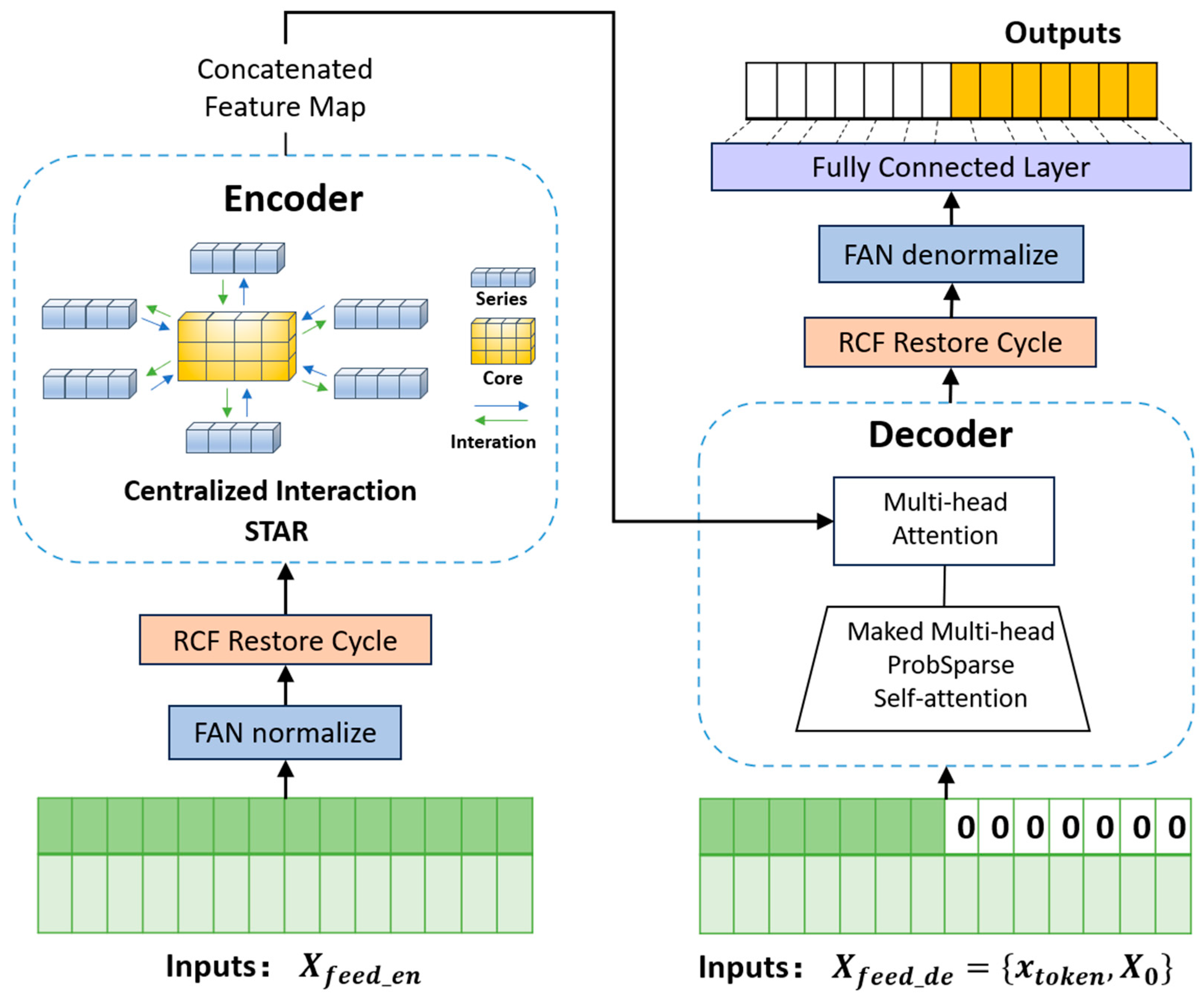
2.5.3. Improved Informer
To address the computational complexity of the Informer model and enhance its robustness against anomalies in the data, we introduced several key modifications:
- Star Aggregate Redistribute Module (STAR): The STAR module, inspired by server–client communication architectures in the Series-cOre Fused Time Series forecaster (SOFTS) model [37], replaces the sparse attention mechanism in Informer’s encoder layer. It introduces a core global representation that acts as a shared intermediary for all channels, facilitating indirect interactions between sequences. This design not only enhances the efficiency of extracting sequence correlations but also overcomes the limitations of traditional distributed interaction modules. The computational complexity of STAR is linear with respect to the number of channels C and sequence length L, i.e., O(CL + CH), where H is the dimension of the representation. This linear complexity ensures superior computational efficiency when handling large-scale data.
- Residual Cycle Forecasting (RCF): A technique designed to capture periodic patterns in time-series data, which is essential for accurate ET0 prediction. The RCF module from the CycleNet model [38] is integrated into the Informer model. It operates through two key steps. 1. Remove Cycle: By learning and removing the periodic components from the original time series, the model can focus on the dynamic features of non-periodic variations. 2. Restore Cycle: The periodic components are reintegrated into the prediction results after forecasting the residuals, thereby capturing both periodic and non-periodic variations. RCF is a plug-and-play module that requires minimal additional parameters. It models the inherent periodic patterns in the data and enhances the model’s adaptability to periodic regularities. The selection of the cycle length (cycle_len) is critical for the effectiveness of RCF. In this study, the cycle length was determined through autocorrelation function (ACF) analysis to ensure accurate detection of periodic features.
- Frequency Adaptive Normalization (FAN): Traditional normalization methods often fail to address non-stationarity in time-series data. FAN, proposed by Weiwei Ye et al. [39], overcomes this limitation by leveraging Fourier transforms to identify and remove dominant frequency components (e.g., trends and seasonal variations) from the data during the normalization step. This process reduces non-stationarity, allowing the model to focus on learning stable features. During the denormalization step, the non-stationary components are reintegrated into the prediction results using a multi-layer perceptron (MLP). FAN effectively handles dynamic trends and seasonal patterns.
By integrating these enhancements, we propose a new long-sequence time-series forecasting model, named Improved Informer. This model combines the efficient information interaction capability of the STAR module, the periodic feature extraction capability of the RCF module, and the adaptive normalization capability of the FAN method. The structure of the Improved Informer model is illustrated in Figure 7.

Figure 7.
Informer-improved model structure diagram.
2.6. Training Configuration
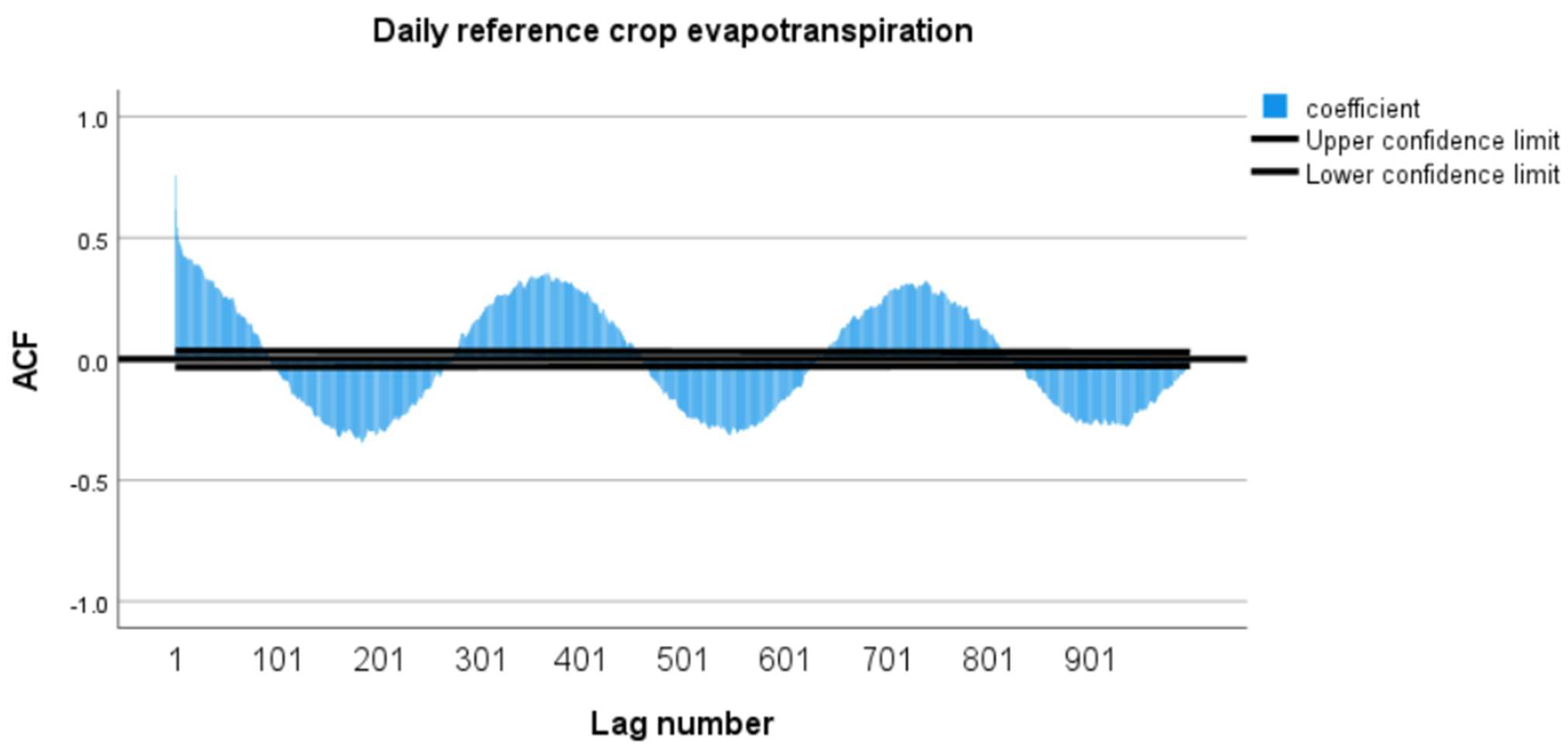
In this study, the Improved Informer model, configured with optimized hyperparameters, was trained to predict daily reference crop evapotranspiration (ET0). To ensure the efficient operation of the RCF module within the Improved Informer model, autocorrelation function (ACF) analysis was used to determine the main cycle length. The ACF analysis result (Figure 8) shows that at the 365-day lag, the autocorrelation coefficient is significantly higher than at other points and exhibits a cyclical fluctuation trend, aligning with the daily frequency characteristics. Therefore, the cycle length parameter (cycle_len) was set to 365 days to capture the annual cycle pattern of the data effectively.
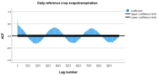
Figure 8.
Results from the autocorrelation analysis of daily reference crop evapotranspiration.
To minimize the impact of differences in parameter settings on model performance and verify the experimental results, we standardized the training parameters for both the Informer original model and the improved version so that an accurate assessment could be achieved of each model’s performance in the forecasting task, laying the foundation for a fair comparison among models. The main parameters for the Informer model improvement experiments are shown in Table 4.
Table 4.
Details of the optimal hyperparameters for training.
In this study, the quantile loss function was uniformly adopted as the core metric for evaluating the model’s prediction performance to quantify the differences between the predicted and actual values. The formula for the quantile loss function is as follows:
where is the actual target value, is the model’s predicted value, and is the quantile coefficient with a range of 0 to 1. When > 0.5, the penalty for underestimation is greater than that for overestimation. Conversely, when < 0.5, the penalty for overestimation is greater. When = 0.5, the quantile loss function reduces to the Mean Absolute Error (MAE) loss. In this experiment, the quantile coefficient was set to 0.45 to measure the model’s performance in the lower median range of predictions.
2.7. Evaluating the Models
To evaluate the prediction performance of the models constructed in this paper, we used several robust evaluation measures including Mean Squared Error (MSE), Root Mean Squared Error (RMSE), Mean Absolute Error (MAE), Coefficient of Determination () and Mean Absolute Percentage Error (MAPE). We selected these indicators to evaluate the model’s accuracy, precision, and overall goodness of fit from different perspectives. The mathematical formulations of these metrics are as follows:
where is the observed value, is the predicted value, is the average of the observed value, and n is the total number of data points.
3. Results
The predictive performance of the models under various scenarios was systematically evaluated using multiple statistical metrics, including MAE, MSE, RMSE, and MAPE. To assess the overall model effectiveness, individual rankings were assigned based on each metric within a given scenario, and an average ranking was computed using the following equation:
where , , , , and are the rankings of MAE, MSE, RMSE, , and MAPE, respectively, within the same scenario.
The Informer model consistently outperformed the LSTM model across all evaluated scenarios, underscoring the effectiveness of its encoder–decoder architecture in capturing complex nonlinear dependencies (Table 5). The Improved Informer model further enhanced its prediction accuracy, with MAE, MSE, RMSE, and MAPE values ranging from 0.065 to 0.083, 0.007 to 0.012, 0.074 to 0.108, 0.993 to 0.995, and 2.913 to 3.566, respectively. These metrics consistently placed Improved Informer among the top two average rankings across different scenarios. In contrast, the original Informer model exhibited MAE, MSE, RMSE, and MAPE values ranging from 0.171 to 0.189, 0.057 to 0.588, 0.241 to 0.261, 0.958 to 0.964, and 7.576 to 8.200, respectively. These results demonstrate the substantial prediction accuracy gains achieved through the architectural enhancements introduced into the Improved Informer model.
Table 5.
Precision of various models in different scenarios.
Scenario-based analysis revealed that prediction accuracy was generally higher in Scenario S1 compared to Scenario S2. This improvement is primarily attributed to the high correlation between soil temperature at 28–100 cm and the maximum temperature at 2 m, which introduced redundancy and negatively impacted the model’s performance in Scenario S2. This observation emphasizes the critical role of feature selection in mitigating multicollinearity and enhancing model generalizability.
Across Scenarios S1–S5, the integration of the RCF mechanism led to noticeable improvements in the predictive accuracy of the Informer model, suggesting that RCF is effective in capturing underlying periodic patterns when the feature dimensionality is relatively low. However, in Scenarios S6–S8, the performance gains associated with RCF were diminished. The increased complexity introduced by higher-dimensional feature sets likely hindered the model’s ability to effectively isolate and leverage periodic components, highlighting the challenges inherent in modeling temporal regularities within high-dimensional datasets.
Similarly, the STAR module, which substitutes the traditional sparse attention mechanism in Informer, demonstrated superior performance in most scenarios. However, its capacity to discern and exploit unique feature interactions was weakened under conditions of high inter-feature correlation. In such cases, redundant features may obscure meaningful relationships, thereby limiting the efficacy of the STAR module in capturing different temporal dependencies.
The introduction of FAN normalization consistently enhanced the model’s performance across all evaluated scenarios. By employing Fourier transforms to identify and eliminate dominant frequency components, FAN effectively addressed the issue of non-stationarity in the time series data. This preprocessing step enabled the model to prioritize stable temporal patterns, thereby substantially improving prediction accuracy—particularly in datasets characterized by pronounced trends and seasonal fluctuations.
These results demonstrate the effectiveness of Scenario S3, which underscores the effectiveness of the five key features—total shortwave radiation, sunshine duration, maximum temperature at 2 m, soil temperature at 28–100 cm, and surface pressure. This scenario achieves high prediction accuracy while minimizing feature redundancy. In contrast, Scenarios S4–S8, which incorporated additional variables, did not yield meaningful improvements in model performance. This outcome highlights that an appropriately curated and concise feature set, as demonstrated in Scenario S3, can optimize both prediction accuracy and model efficiency.
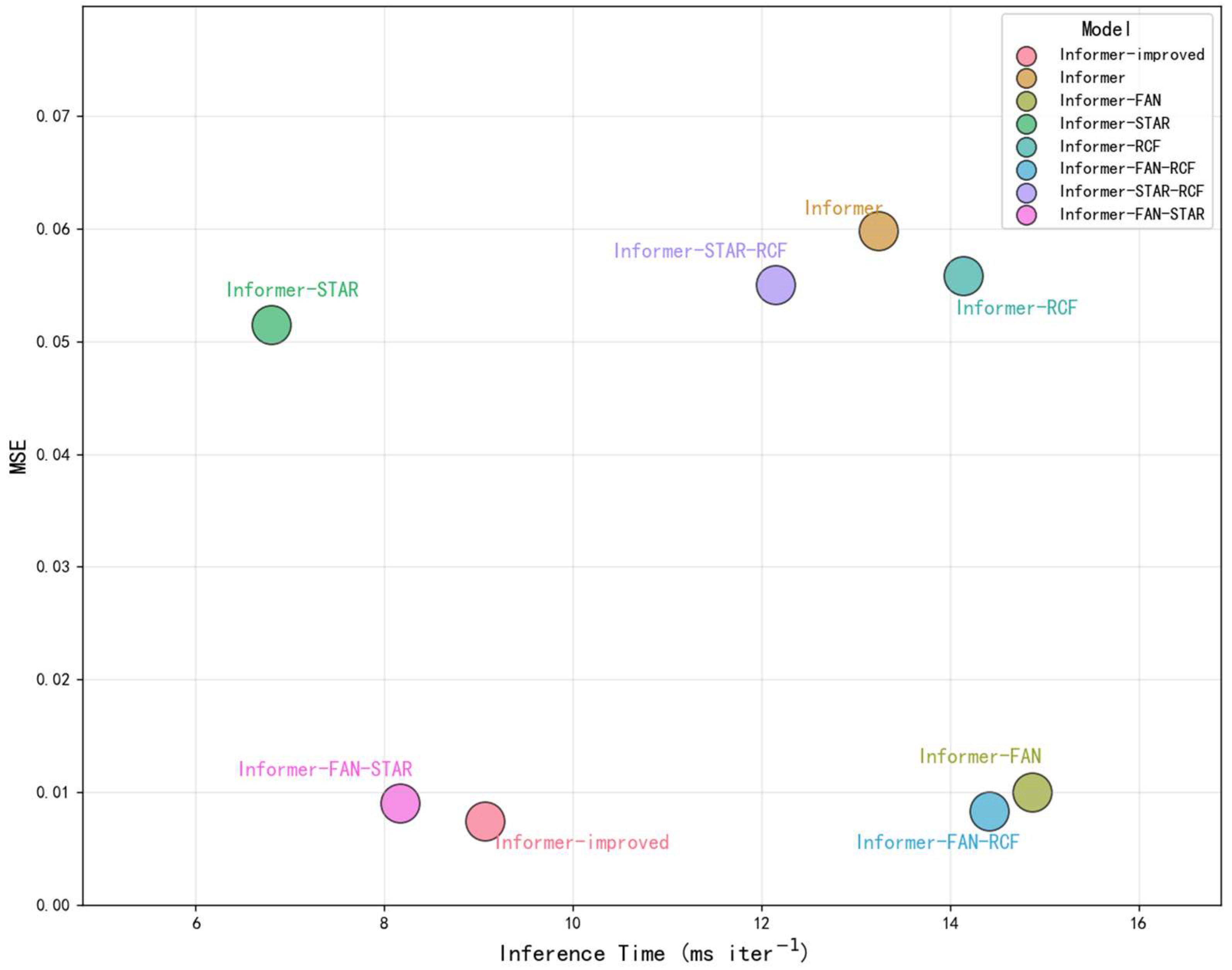
Figure 9 depicts the relationship between inference time and MSE for the Informer model and its improved variants in Scenario S3. The integration of the STAR module markedly reduced computational complexity and time consumption compared to the original Informer’s sparse attention mechanism, thereby enhancing model efficiency. The addition of the RCF module yielded further performance improvements with only a marginal increase in inference time, demonstrating a favorable balance between computational cost and predictive gain. Similarly, the incorporation of FAN normalization led to a significant improvement in prediction accuracy while incurring only a slight computational overhead. These results suggest that the STAR mechanism is particularly well-suited for applications prioritizing high computational efficiency, whereas FAN normalization is more effective in scenarios emphasizing predictive accuracy. The RCF module contributes meaningfully when periodic patterns are present, offering targeted benefits in specific temporal contexts. Collectively, the integration of the STAR, RCF, and FAN modules results in a robust and optimized framework. In Scenario S3, the Improved Informer model achieved the lowest MSE and demonstrated a more efficient inference time, underscoring its superior performance and practical applicability.
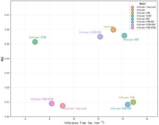
Figure 9.
Model Performance Comparison: Inference Time and MSE Analysis.
In Figure 10, it can be observed that Improved Informer, Informer-FAN-STAR and Informer-FAN-RCF outperformed the other models in Scenario S3. These results provide further empirical evidence that the integration of FAN normalization with the STAR and RCF modules substantially enhances the model’s capacity to capture complex temporal dependencies and extract meaningful patterns from time series data. The synergistic effect of these modules significantly improved the overall prediction accuracy.
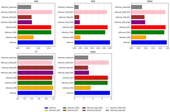
Figure 10.
Performance Chart of Informer and Its Improved Model in Scenario S3.
Figure 11 compares the predicted ET0 values generated by the Improved Informer model with the calculated ET0 values derived from the FAO-56 Penman–Monteith equation in Scenario S3. It demonstrates that the Improved Informer model closely follows the overall temporal trend of ET0, capturing both seasonal fluctuations and short-term variations with low prediction error. The model effectively tracks the true ET0 values, including major peaks and troughs, across most time points.
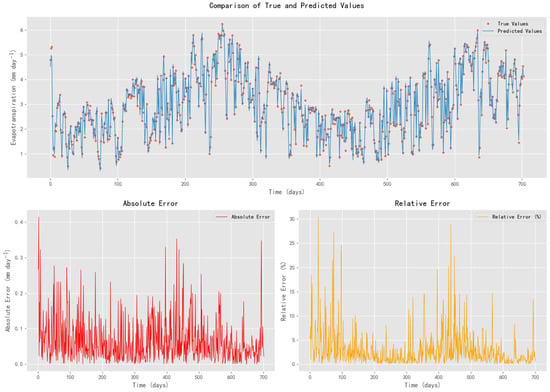
Figure 11.
Comparison of Improved Informer Model Prediction Values and Evapotranspiration Calculation Values in Scenario S3.
However, discrepancies between the predicted and actual values are more evident during abrupt changes and local extremes in ET0. These deviations appear to be non-systematic, suggesting that the model does not exhibit consistent bias. The absolute error varies over time but remains within a low range for the majority of observations. During periods of elevated ET0, the absolute error may reach up to 0.4 mm, indicating potential challenges in model responsiveness to rapid changes or high evapotranspiration conditions.
The relative error remains generally low, typically below 10%, indicating a slight proportional deviation between the predicted and actual values. However, the relative errors occasionally exceed 20% (and even reach 30%) at specific time points, particularly when the ET0 values are low. This points to limitations in the model performance under low ET0 conditions, where minor absolute errors can translate into relatively larger proportional discrepancies.
Overall, the Improved Informer model exhibits robust performance in capturing the trend and variability of ET0, with both absolute and relative errors remaining low for most of the time. These findings validate its utility for precision irrigation applications, while also highlighting opportunities for further refinement in handling abrupt fluctuations and low ET0 values.
4. Conclusions
This study addresses the challenge of predicting ET0 for precision irrigation by introducing an Improved Informer model. By integrating MIC-based feature selection with optimization modules—RCF, STAR and FAN—the Improved Informer model achieved higher prediction accuracy and computational efficiency.
The experimental results showed that in Scenario S3, the Improved Informer model outperformed both LSTM and the original Informer when using five key features: total shortwave radiation, sunshine duration, maximum temperature at 2 m, soil temperature at 28–100 cm, and surface pressure. The model reduced MAE to 0.065 (compared to 0.637 for LSTM and 0.171 for Informer) and MSE to 0.007 (compared to 0.678 for LSTM and 0.060 for Informer). Additionally, it decreased the inference time by 31% relative to the original Informer, demonstrating significant efficiency improvements.
The Improved Informer model incorporates several key enhancements. The RCF module mitigates periodic noise interference by modeling cycles in evapotranspiration data, thereby reducing performance degradation. For nonstationary time series, the FAN module dynamically adapts to temporal and seasonal variations, improving prediction stability under heterogeneous environmental conditions. A significant advancement is the STAR module, which optimizes long-term dependency modeling through efficient sequence interactions while maintaining low computational overhead—especially valuable for large-scale agricultural datasets.
Beyond architectural enhancements, the MIC-driven feature selection yields a parsimonious feature subset comprising five key variables: total shortwave radiation, sunshine duration, maximum temperature at 2 m, soil temperature at 28–100 cm, and surface pressure. This demonstrates that reducing the input dimensionality does not compromise performance. Instead, it strikes a balance between model simplicity and high accuracy while significantly enhancing computational efficiency.
While this feature set differs from the complete set of variables typically used in the Penman–Monteith equation, it still captures key physical components of evapotranspiration. For instance, total shortwave radiation and sunshine duration contribute to estimating the net radiation, the maximum temperature influences the calculation of vapor pressure, and the surface pressure affects humidity-related processes. The exclusion of wind speed and relative humidity suggests that the deep learning model may infer their effects through interactions among the selected features.
Future research could further refine the model and evaluate its adaptability and generalization across broader regions. Methodologically, incorporating physically based constraints from the Penman–Monteith framework alongside multisource data fusion techniques could enhance both model interpretability and generalizability. Additionally, techniques like Shapley Additive Explanations (SHAP) analysis could provide deeper insights into how the model captures key ET0 processes. Geographically, validating the framework across diverse agroclimatic zones (e.g., arid Mediterranean basins vs. tropical monsoonal regions) would test its robustness to spatial heterogeneity. Operationally, incorporating adaptive mechanisms to account for region-specific factors (e.g., irrigation practices and soil hydrology) could enhance the model’s applicability in global precision agriculture systems.
Author Contributions
Conceptualization, J.P. and L.Y.; methodology, J.P., B.Z. and L.Y.; software, J.P. and L.Y.; validation, J.P., L.Y., B.Z. and J.Z.; data curation, J.P., L.Y. and B.Z.; writing—original draft preparation, J.P.; writing—review and editing, J.P., L.Y. and B.Z.; visualization, J.P., L.Y., B.Z. and J.Z. All authors have read and agreed to the published version of the manuscript.
Funding
This research was funded by The 2024 Guangdong Province “Hundreds of Thousands of Projects” Rural Science and Technology Commissioner Project (KTP20240367) and The Project of Collaborative Innovation Center of GDAAS (XTXM202201).
Institutional Review Board Statement
Not applicable.
Data Availability Statement
The datasets were obtained from ERA5 hourly data on single levels from 1940 to the present. Copernicus Climate Change Service (C3S) Climate Data Store (CDS). (https://cds.climate.copernicus.eu/datasets/reanalysis-era5-single-levels?tab=overview, accessed on 3 December 2024) (https://doi.org/10.24381/cds.adbb2d47).
Conflicts of Interest
The authors declare no conflicts of interest.
References
- Ministry of Water Resources. 2023. China Water Resources Bulletin. Available online: http://www.mwr.gov.cn/sj/tjgb/szygb/ (accessed on 14 June 2024).
- Bwire, D.; Watanabe, F.; Suzuki, S.; Suzuki, K. Improving Irrigation Water Use Efficiency and Maximizing Vegetable Yields with Drip Irrigation and Poly-Mulching: A Climate-Smart Approach. Water 2024, 16, 3458. [Google Scholar] [CrossRef]
- Mgendi, G. Unlocking the potential of precision agriculture for sustainable farming. Discov. Agric. 2024, 2, 87. [Google Scholar] [CrossRef]
- Ali, M.; Nayahi, J.V.; Abdi, E.; Ghorbani, M.A.; Mohajeri, F.; Farooque, A.A.; Alamery, S. Improving daily reference evapotranspiration forecasts: Designing AI-enabled recurrent neural networks based long short-term memory. Ecol. Inform. 2025, 85, 102995. [Google Scholar] [CrossRef]
- Buri, E.S.; Keesara, V.R.; Loukika, K.; Sridhar, V. An Integrated Framework for Optimal Allocation of Land and Water Resources in an Agricultural Dominant Basin. Water Resour. Manag. 2024, 39, 1435–1451. [Google Scholar] [CrossRef]
- Acharki, S.; Raza, A.; Vishwakarma, D.K.; Amharref, M.; Bernoussi, A.S.; Singh, S.K.; Al-Ansari, N.; Dewidar, A.Z.; Al-Othman, A.A.; Mattar, M.A. Comparative assessment of empirical and hybrid machine learning models for estimating daily reference evapotranspiration in sub-humid and semi-arid climates. Sci. Rep. 2025, 15, 2542. [Google Scholar] [CrossRef] [PubMed]
- Habeeb, R.; Almazah, M.M.A.; Hussain, I.; Al-Rezami, A.Y.; Raza, A.; Ray, R.L. Improving Reference Evapotranspiration Predictions with Hybrid Modeling Approach. Earth Syst. Environ. 2025. [Google Scholar] [CrossRef]
- Kong, X.; Chen, Z.; Liu, W.; Ning, K.; Zhang, L.; Marier, S.M.; Liu, Y.; Chen, Y.; Xia, F. Deep Learning for Time Series Forecasting: A Survey. Int. J. Mach. Learn. Cybern. 2025. [Google Scholar] [CrossRef]
- Del-Coco, M.; Leo, M.; Carcagnì, P. Machine Learning for Smart Irrigation in Agriculture: How Far along Are We? Information 2024, 15, 306. [Google Scholar] [CrossRef]
- Kumar, D.; Adamowski, J.; Suresh, R.; Ozga-Zielinski, B. Estimating evapotranspiration using an extreme learning machine model: Case study in north Bihar, India. J. Irrig. Drain. Eng. 2016, 142, 04016032. [Google Scholar] [CrossRef]
- Talib, A.; Desai, A.R.; Huang, J.; Griffis, T.J.; Reed, D.E.; Chen, J. Evaluation of prediction and forecasting models for evapotranspiration of agricultural lands in the Midwest US. J. Hydrol. 2021, 600, 126579. [Google Scholar] [CrossRef]
- Dolaptsis, K.; Pantazi, X.E.; Paraskevas, C.; Arslan, S.; Tekin, Y.; Bantchina, B.B.; Ulusoy, Y.; Gündoğdu, K.S.; Qaswar, M.; Bustan, D.; et al. A Hybrid LSTM Approach for Irrigation Scheduling in Maize Crop. Agriculture 2024, 14, 210. [Google Scholar] [CrossRef]
- Abdel-Fattah, M.K.; Kotb Abd-Elmabod, S.; Zhang, Z.; Merwad, A.-R.M.A. Exploring the Applicability of Regression Models and Artificial Neural Networks for Calculating Reference Evapotranspiration in Arid Regions. Sustainability 2023, 15, 15494. [Google Scholar] [CrossRef]
- Wu, Y.; Hu, F.; Yue, C.; Sun, S. Residual-time gated recurrent unit. Neurocomputing 2025, 624, 129396. [Google Scholar] [CrossRef]
- Umutoni, L.; Samadi, V. Application of machine learning approaches in supporting irrigation decision making: A review. Agric. Water Manag. 2024, 294, 108710. [Google Scholar] [CrossRef]
- Liyew, C.M.; Di Nardo, E.; Ferraris, S.; Meo, R.J.A.a.S. Hyperparameter Optimization of Machine Learning Models for Predicting Actual Evapotranspiration. Available online: https://ssrn.com/abstract=5123630 (accessed on 4 February 2025).
- Gao, Z.; Gao, Z.; Zhang, X.; Cao, S.; Zhou, B.; Liu, Y.; Liu, D.; Liu, W. Integrated Seasonal-Trend Decomposition Using Loess for Multi-Head Self-Attention Mechanism and Bidirectional Long Short-Term Memory Based Reference Evapotranspiration Prediction. Available online: https://ssrn.com/abstract=5118476 (accessed on 1 January 2025).
- Kandadi, T.; Shankarlingam, G. Drawbacks of Lstm Algorithm: A Case Study. Available online: https://ssrn.com/abstract=5080605 (accessed on 3 January 2025).
- Vaswani, A.; Shazeer, N.; Parmar, N.; Uszkoreit, J.; Jones, L.; Gomez, A.N.; Polosukhin, I. Attention is all you need. In Proceedings of the 31st Conference on Neural Information Processing Systems (NIPS 2017), Long Beach, CA, USA, 4–9 December 2017; Volume 30. [Google Scholar]
- Abed, M.; Imteaz, M.A.; Ahmed, A.N.; Huang, Y.F. A novel application of transformer neural network (TNN) for estimating pan evaporation rate. Appl. Water Sci. 2023, 13, 31. [Google Scholar] [CrossRef]
- Zhou, H.; Zhang, S.; Peng, J.; Zhang, S.; Li, J.; Xiong, H.; Zhang, W. Informer: Beyond efficient transformer for long sequence time-series forecasting. Proc. Aaai Conf. Artif. Intell. 2021, 35, 11106–11115. [Google Scholar] [CrossRef]
- Shang, J.; Zhao, B.; Hua, H.; Wei, J.; Qin, G.; Chen, G. Application of Informer Model Based on SPEI for Drought Forecasting. Atmosphere 2023, 14, 951. [Google Scholar] [CrossRef]
- Nagappan, M.; Gopalakrishnan, V.; Alagappan, M. Prediction of reference evapotranspiration for irrigation scheduling using machine learning. Hydrol. Sci. J. 2020, 65, 2669–2677. [Google Scholar] [CrossRef]
- Chen, P.; Li, C.; Chen, S.; Li, Z.; Zhang, H.; Zhao, C. Tea Cultivation Suitability Evaluation and Driving Force Analysis Based on AHP and Geodetector Results: A Case Study of Yingde in Guangdong, China. Remote Sens. 2022, 14, 2412. [Google Scholar] [CrossRef]
- Qi, N.; Yang, H.; Shao, G.; Chen, R.; Wu, B.; Xu, B.; Feng, H.; Yang, G.; Zhao, C. Mapping tea plantations using multitemporal spectral features by harmonised Sentinel-2 and Landsat images in Yingde, China. Comput. Electron. Agric. 2023, 212, 108108. [Google Scholar] [CrossRef]
- Martin Nascimento, G.F.; Wurtz, F.; Kuo-Peng, P.; Delinchant, B.; Jhoe Batistela, N. Outlier Detection in Buildings’ Power Consumption Data Using Forecast Error. Energies 2021, 14, 8325. [Google Scholar] [CrossRef]
- Liu, C.; Liu, Z.; Yuan, J.; Wang, D.; Liu, X. Urban Water Demand Prediction Based on Attention Mechanism Graph Convolutional Network-Long Short-Term Memory. Water 2024, 16, 83. [Google Scholar] [CrossRef]
- Dinpashoh, Y.; Jhajharia, D.; Fakheri-Fard, A.; Singh, V.P.; Kahya, E. Trends in reference crop evapotranspiration over Iran. J. Hydrol. 2011, 399, 422–433. [Google Scholar] [CrossRef]
- Reshef, D.N.; Reshef, Y.A.; Finucane, H.K.; Grossman, S.R.; McVean, G.; Turnbaugh, P.J.; Lander, E.S.; Mitzenmacher, M.; Sabeti, P.C. Detecting novel associations in large data sets. Science 2011, 334, 1518–1524. [Google Scholar] [CrossRef] [PubMed]
- Chen, Z.; Sun, S.; Wang, Y.; Wang, Q.; Zhang, X. Temporal convolution-network-based models for modeling maize evapotranspiration under mulched drip irrigation. Comput. Electron. Agric. 2020, 169, 105206. [Google Scholar] [CrossRef]
- Hochreiter, S.; Schmidhuber, J. Long short-term memory. Neural Comput. 1997, 9, 1735–1780. [Google Scholar] [CrossRef]
- Gers, F.A.; Schmidhuber, J.; Cummins, F. Learning to forget: Continual prediction with LSTM. Neural Comput. 2000, 12, 2451–2471. [Google Scholar] [CrossRef]
- Wang, Y.; Zha, Y. Comparison of transformer, LSTM and coupled algorithms for soil moisture prediction in shallow-groundwater-level areas with interpretability analysis. Agric. Water Manag. 2024, 305, 109120. [Google Scholar] [CrossRef]
- Zhu, Q.; Han, J.; Chai, K.; Zhao, C. Time Series Analysis Based on Informer Algorithms: A Survey. Symmetry 2023, 15, 951. [Google Scholar] [CrossRef]
- Yu, F.; Koltun, V.; Funkhouser, T. Dilated residual networks. In Proceedings of the 2017 IEEE Conference on Computer Vision and Pattern Recognition, CVPR 2017, Honolulu, HI, USA, 21–26 July 2017; pp. 636–644. [Google Scholar]
- Xu, Y.; Zhao, J.; Wan, B.; Cai, J.; Wan, J. Flood Forecasting Method and Application Based on Informer Model. Water 2024, 16, 765. [Google Scholar] [CrossRef]
- Han, L.; Chen, X.-Y.; Ye, H.-J.; Zhan, D.-C. Softs: Efficient multivariate time series forecasting with series-core fusion. arXiv 2024, arXiv:2404.14197. [Google Scholar]
- Lin, S.; Lin, W.; Hu, X.; Wu, W.; Mo, R.; Zhong, H.J. Cyclenet: Enhancing time series forecasting through modeling periodic patterns. Adv. Neural Inf. Process. Syst. 2025, 37, 106315–106345. [Google Scholar]
- Ye, W.; Deng, S.; Zou, Q.; Gui, N. Frequency adaptive normalization for non-stationary time series forecasting. Adv. Neural Inf. Process. Syst. 2025, 37, 31350–31379. [Google Scholar]


Disclaimer/Publisher’s Note: The statements, opinions and data contained in all publications are solely those of the individual author(s) and contributor(s) and not of MDPI and/or the editor(s). MDPI and/or the editor(s) disclaim responsibility for any injury to people or property resulting from any ideas, methods, instructions or products referred to in the content. |
© 2025 by the authors. Licensee MDPI, Basel, Switzerland. This article is an open access article distributed under the terms and conditions of the Creative Commons Attribution (CC BY) license (https://creativecommons.org/licenses/by/4.0/).