
A Programmable Aerial Multispectral Camera System for In-Season Crop Biomass and Nitrogen Content Estimation

Abstract
:1. Introduction
2. Materials and Methods


| Component | Parameter | Value | Parameter | Value |
|---|---|---|---|---|
| D3 platform | Name | VRmD3MFC | ||
| CPU | 1-GHz ARM Cortex-A8 Core | Memory | 32 GB flash | |
| DSP | 700-MHz C674x | RAM | 2 GB DDR3-800 | |
| Image sensor | Name | Aptina MT9V024 | ||
| Size | 4.51 mm (H) × 2.88 mm (V) | Pixel size | 6 μm × 6 μm | |
| Resolution | 752 px (H) × 480 px (V) | Shutter | Global | |
| Dynamic range | 10 bit (1024) | Quantum eff. | ~49%, 47.5%, 44%, 41% | |
| Type | CMOS monochrome (1/3 in) | (670, 700, 740, 780 nm) | ||
| Lens system | Focal length | 3.6 mm | F-number | 1.8 |
| Filter | Type | Bandpass interference filter | ||
| Wavelengths | 670, 700, 740, 780 nm | Tmax | ≥70, typically 85% | |
| Center | ±2 nm | FWHM | 10 ±2 nm | |
| Luminosity | Name | TSL 2561 | ||
| Sensitivity | ~350–900 nm | Dynamic range | 0.1–40,000 lx |
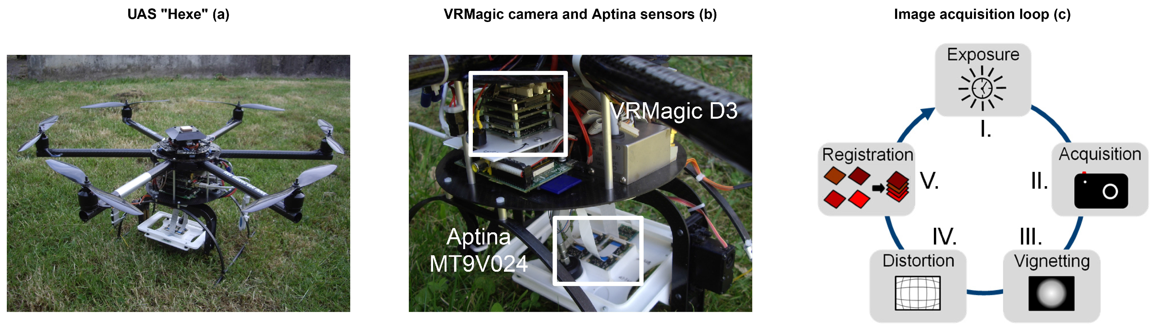
2.1. Image Acquisition Loop
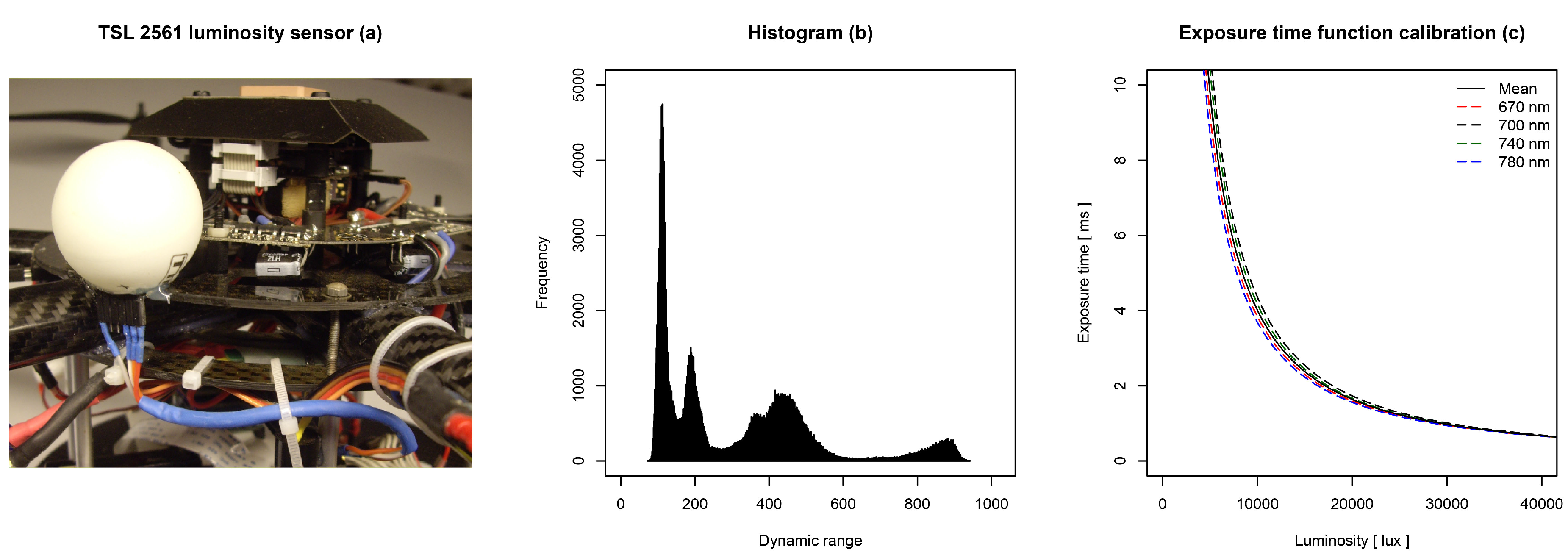
2.1.1. Exposure Time

2.1.2. Sensitivity, Vignetting and Lens Distortion
2.1.3. Image-To-Image Registration
2.2. Carrier Platform
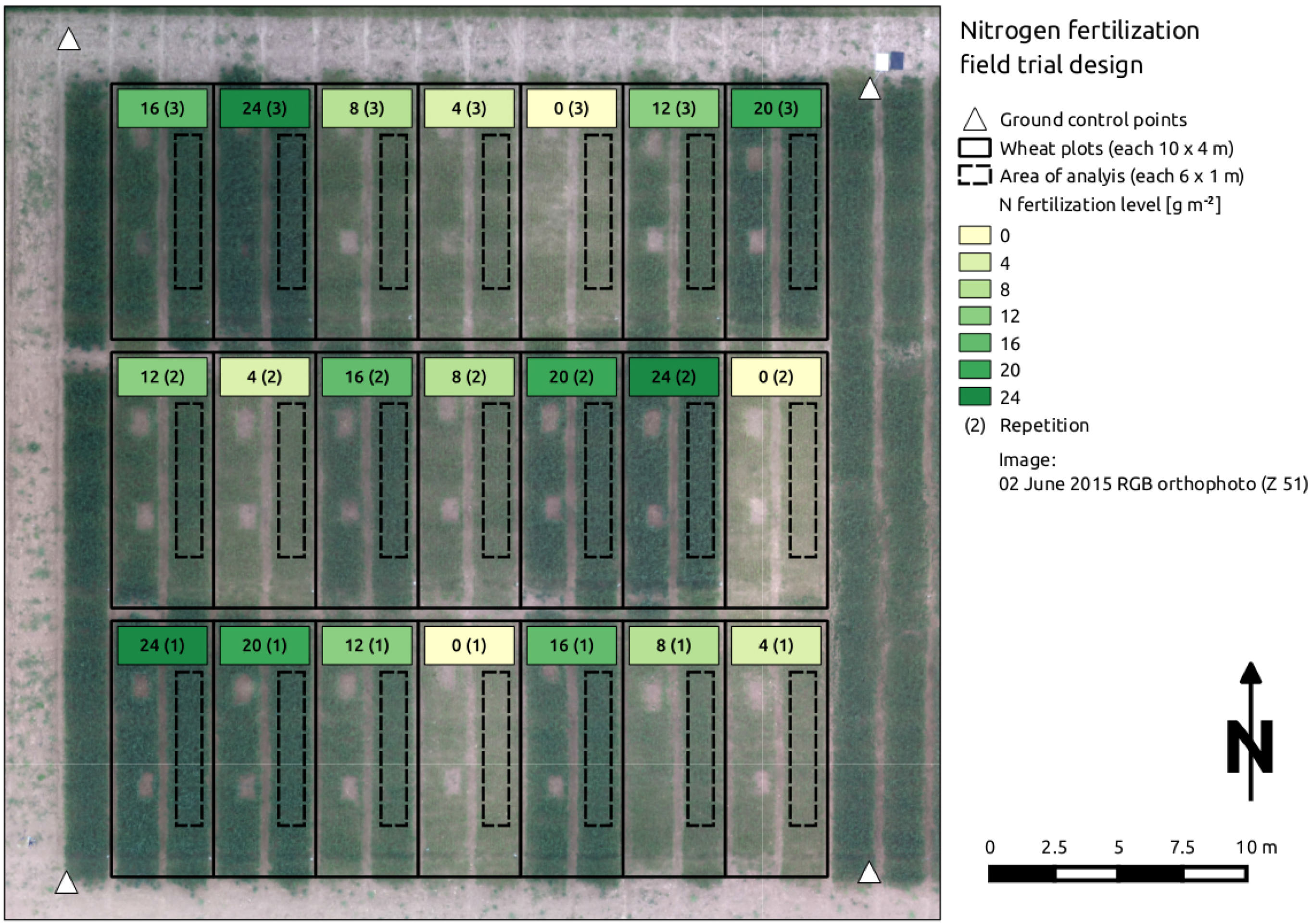
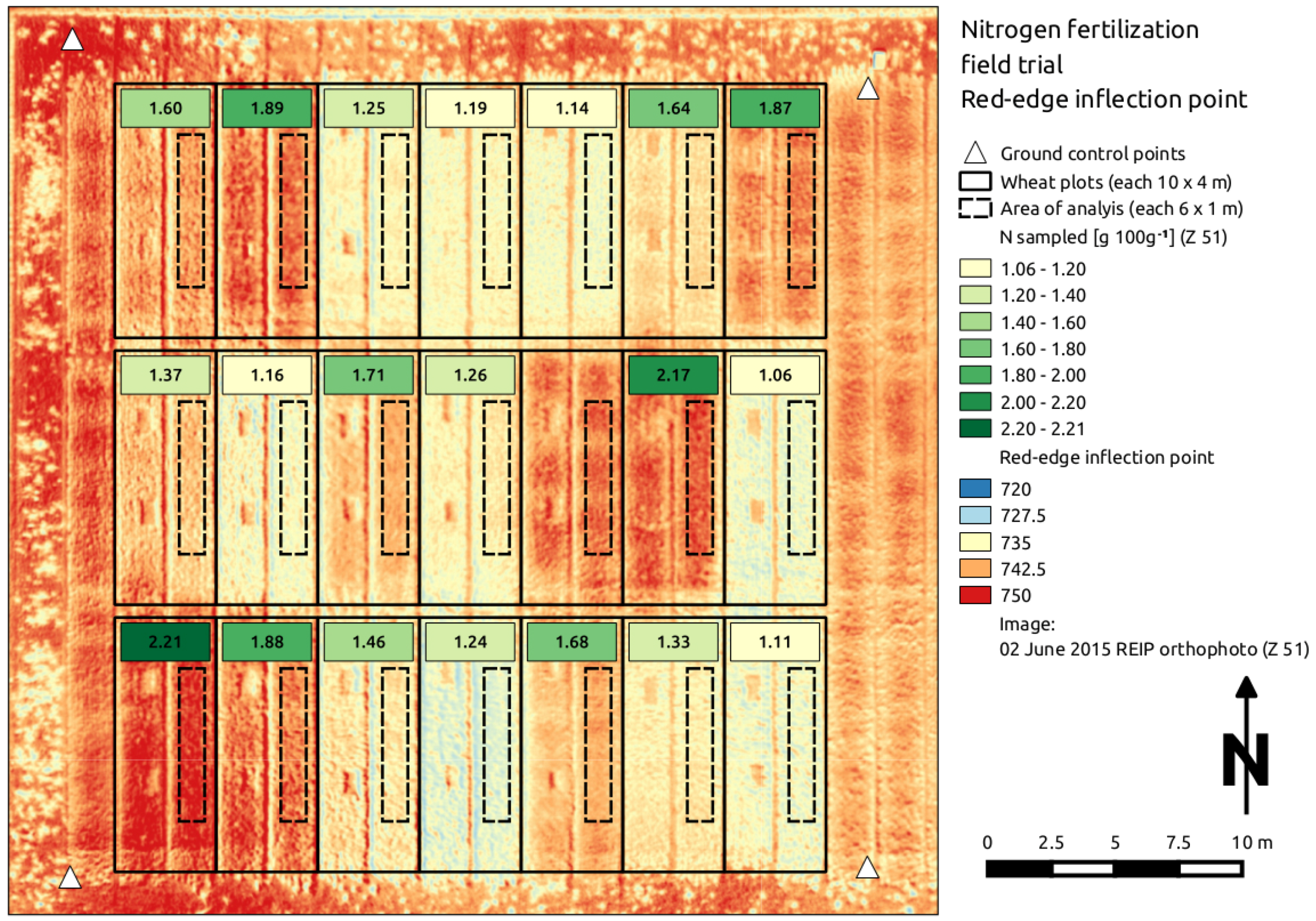
2.3. Field Trial

| Date | Z | N | N | N | N (g·m) | N | N | N | P (mm·m) |
|---|---|---|---|---|---|---|---|---|---|
| 20 March 2015 | 20 | 0 | 2 | 3 | 4 | 6 | 8 | 10 | |
| 24 April 2015 | 31 | 0 | 2 | 3 | 4 | 6 | 8 | 10 | 43.8 |
| 26 May 2015 | 39–41 | 70.7 | |||||||
| 2 June 2015 | 51 | 79.7 | |||||||
| 5 June 2015 | 51 | 0 | 0 | 2 | 4 | 4 | 4 | 4 | 79.7 |
| 10 June 2015 | 61 | 46.0 | |||||||
| 17 June 2015 | 69 | 46.4 | |||||||
| 5 August 2015 | 90 | 104.3 |
2.4. Measurements
| Date | Z | n | A (m) | G | R (m·px) | T | W | Ze | Az | S (m·s) |
|---|---|---|---|---|---|---|---|---|---|---|
| 26 May 2015 | 39–41 | 121 | 25 | 6 | 0.04 | 10–11 a.m. | clear sky | 44 | 114 | 2 |
| 2 June 2015 | 51 | 128 | 25 | 6 | 0.04 | 10–11 a.m. | clear sky | 43 | 113 | 3 |
| 10 June 2015 | 61 | 132 | 25 | 6 | 0.04 | 2–3 p.m. | clear sky | 29 | 212 | 2 |
| 17 June 2015 | 69 | 135 | 25 | 6 | 0.04 | 2–3 p.m. | clear sky | 29 | 212 | 1 |
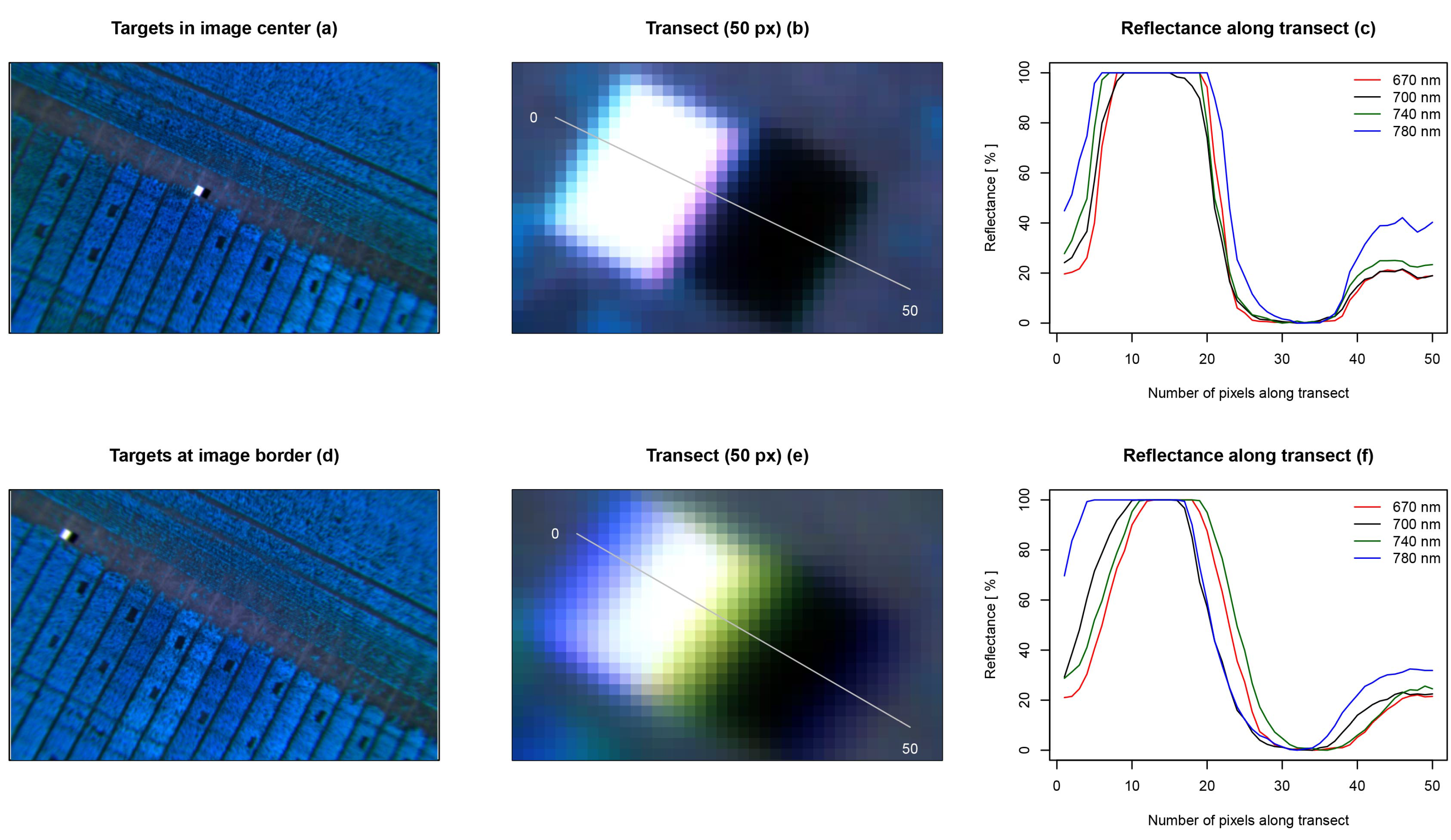
2.5. Image Processing
2.6. Regression Analysis
3. Results
3.1. Image Acquisition Loop

3.2. Measurements
| Variable | Z | Minimum | Mean | Maximum | SD |
|---|---|---|---|---|---|
| Biomass (DM) (g·m) | 39–41 | 91.9 | 381.8 | 665.5 | 130.13 |
| 51 | 241.8 | 512.1 | 848.0 | 165.17 | |
| 61 | 444.4 | 955.5 | 1447.3 | 324.26 | |
| 69 | 486.1 | 1351.3 | 2076.0 | 432.97 | |
| N content (g 100 g) | 39–41 | 1.1 | 1.5 | 2.0 | 0.30 |
| 51 | 1.1 | 1.5 | 2.2 | 0.36 | |
| 61 | 0.9 | 1.2 | 1.9 | 0.28 | |
| 69 | 0.9 | 1.3 | 1.7 | 0.24 | |
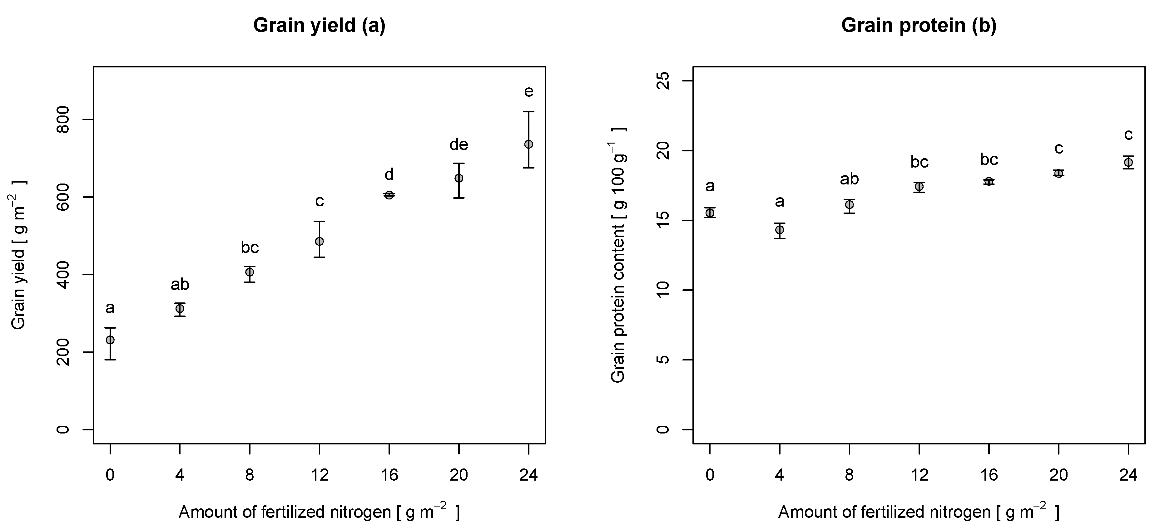
| Grain yield (g·m) | 90 | 180.4 | 489.7 | 820.7 | 178.74 |
| Grain protein content (g 100 g) | 90 | 13.7 | 17.0 | 19.6 | 1.65 |

3.3. Image Processing

3.4. Regression Analysis
| DV | IDV | Z | n | R | RMSE | RMSE | Bias | RMSEV |
|---|---|---|---|---|---|---|---|---|
| Biomass (DM) (g·m) | NDVI | 39–41 | 21 | 0.78 | 59.9 | 15.7 | 0 | 66.4 |
| 51 | 20 | 0.85 | 62.8 | 12.3 | 0 | 69.1 | ||
| 61 | 21 | 0.72 | 168.1 | 17.6 | 0 | 185.4 | ||
| 69 | 20 | 0.84 | 166.8 | 12.3 | 0 | 179.8 | ||
| REIP | 39–41 | 21 | 0.74 | 65.1 | 17.1 | 0 | 73.0 | |
| 51 | 20 | 0.81 | 69.7 | 13.6 | 0 | 80.4 | ||
| 61 | 21 | 0.77 | 150.8 | 15.8 | 0 | 167.6 | ||
| 69 | 20 | 0.70 | 230.6 | 17.1 | 0 | 253.7 | ||
| N content (g 100 g) | NDVI | 39–41 | 21 | 0.75 | 0.15 | 10.2 | 0 | 0.17 |
| 51 | 20 | 0.73 | 0.18 | 11.9 | 0 | 0.20 | ||
| 61 | 21 | 0.63 | 0.17 | 14.3 | 0 | 0.19 | ||
| 69 | 20 | 0.53 | 0.16 | 12.5 | 0 | 0.19 | ||
| REIP | 39–41 | 21 | 0.83 | 0.12 | 8.3 | 0 | 0.13 | |
| 51 | 20 | 0.89 | 0.11 | 7.6 | 0 | 0.13 | ||
| 61 | 21 | 0.81 | 0.12 | 10.3 | 0 | 0.14 | ||
| 69 | 20 | 0.58 | 0.15 | 11.7 | 0 | 0.17 |

| DV | IDV | Z | n | R | RMSE | RMSE | Bias | RMSEV |
|---|---|---|---|---|---|---|---|---|
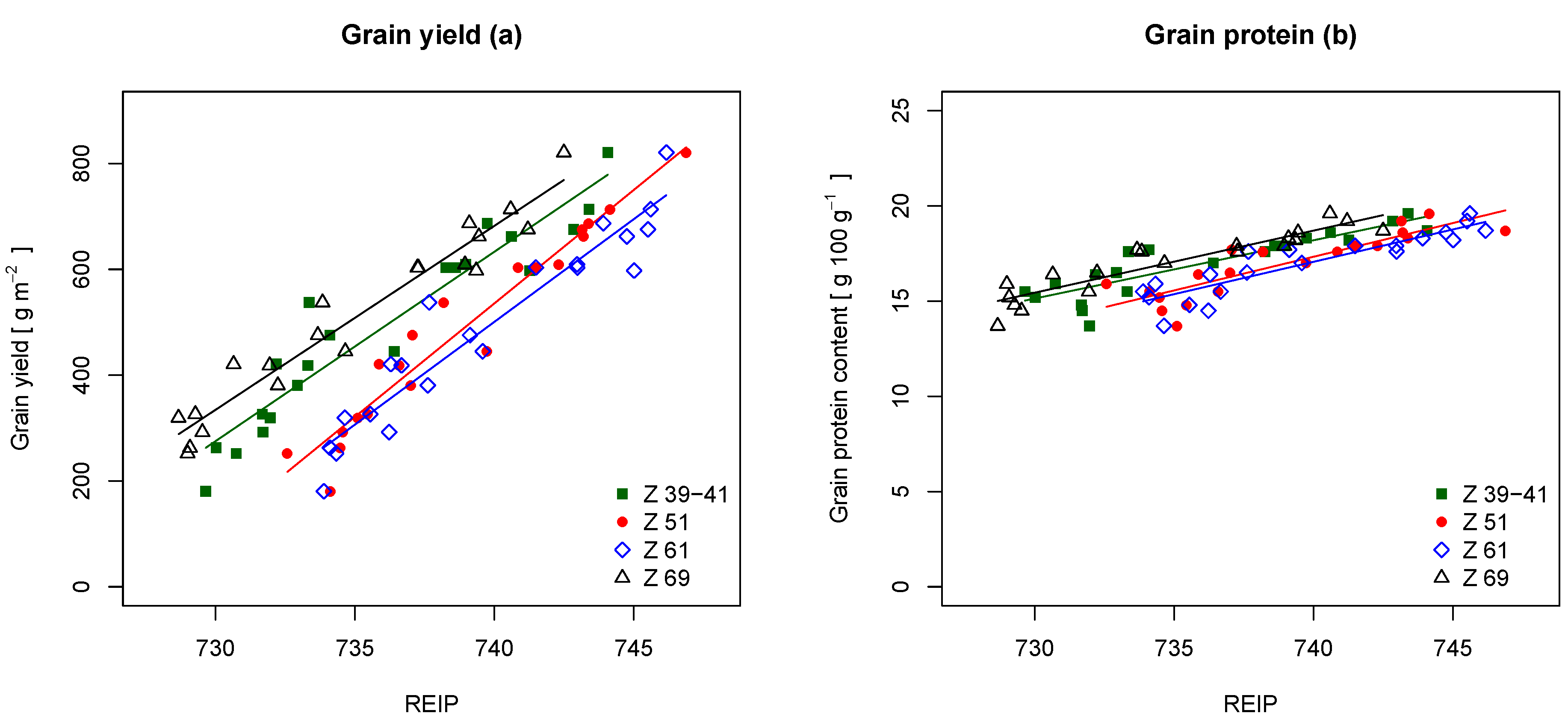
| Grain yield (g·m) | NDVI | 39–41 | 21 | 0.89 | 56.7 | 11.6 | 0 | 64.5 |
| 51 | 21 | 0.89 | 59.1 | 12.1 | 0 | 65.8 | ||
| 61 | 21 | 0.90 | 54.1 | 11.0 | 0 | 60.7 | ||
| 69 | 21 | 0.91 | 53.5 | 10.9 | 0 | 59.9 | ||
| REIP | 39–41 | 21 | 0.90 | 54.8 | 11.2 | 0 | 60.4 | |
| 51 | 21 | 0.92 | 48.3 | 9.9 | 0 | 53.1 | ||
| 61 | 21 | 0.91 | 52.9 | 10.8 | 0 | 58.7 | ||
| 69 | 21 | 0.94 | 44.2 | 9.0 | 0 | 49.2 | ||
| Grain protein content (g 100 g) | NDVI | 39–41 | 21 | 0.72 | 0.86 | 5.1 | 0 | 0.96 |
| 51 | 21 | 0.71 | 0.87 | 5.1 | 0 | 0.99 | ||
| 61 | 21 | 0.72 | 0.85 | 5.0 | 0 | 0.95 | ||
| 69 | 21 | 0.74 | 0.83 | 4.9 | 0 | 0.94 | ||
| REIP | 39–41 | 21 | 0.77 | 0.77 | 4.5 | 0 | 0.84 | |
| 51 | 21 | 0.76 | 0.79 | 4.7 | 0 | 0.89 | ||
| 61 | 21 | 0.82 | 0.69 | 4.1 | 0 | 0.76 | ||
| 69 | 21 | 0.86 | 0.61 | 3.6 | 0 | 0.68 |

4. Discussion
4.1. Image Acquisition Loop
4.2. Measurements
4.3. Image Processing
4.4. Regression Analysis
5. Conclusions
Acknowledgments
Author Contributions
Conflicts of Interest
References
- Matson, P.A.; Parton, W.J.; Power, A.G.; Swift, M.J. Agricultural Intensification and Ecosystem Properties. Science 1997, 277, 504–509. [Google Scholar] [CrossRef] [PubMed]
- Spiertz, J.H.J. Nitrogen, sustainable agriculture and food security. A review. Agron. Sustain. Dev. 2010, 30, 43–55. [Google Scholar] [CrossRef]
- Cameron, K.; Di, H.; Moir, J. Nitrogen losses from the soil/plant system: A review. Ann. Appl. Biol. 2013, 162, 145–173. [Google Scholar] [CrossRef]
- OECD. Eutrophication of Waters. Monitoring, Assessment and Control; Final Report; Organization for Economic Co-Operation and Development (OECD): Paris, France, 1982. [Google Scholar]
- WHO. Guidelines for Drinking-Water Quality, Volume 1: Recommendations; World Health Organization (WHO): Geneva, Switzerland, 1984. [Google Scholar]
- Aufhammer, W. Getreide- und Andere Körnerfruchtarten: Bedeutung, Nutzung und Anbau; Ulmer Verlag, UTB für Wissenschaft: Stuttgart, Germany, 1998. [Google Scholar]
- McKenna, P. Report on the Commission Reports on the Implementation of Council Directive 91/676/EEC. Committee on the Environment, Public Health and Consumer Protection (A4-0284/98); European Commission: Brussels, Belgium, 1998. [Google Scholar]
- Mosier, A.; Kroeze, C.; Nevison, C.; Oenema, O.; Seitzinger, S.; van Cleemput, O. Closing the global N2O budget: Nitrous oxide emissions through the agricultural nitrogen cycle. Nutr. Cycl. Agroecosyst. 1998, 52, 225–248. [Google Scholar] [CrossRef]
- Ellen, J.; Spiertz, J. Effects of rate and timing of nitrogen dressings on grain field formation of winter wheat (Triticum aestivum L.). Fertil. Res. 1980, 1, 177–190. [Google Scholar] [CrossRef]
- Weber, E.; Graeff, S.; Koller, W.D.; Hermann, W.; Merkt, N.; Claupein, W. Impact of nitrogen amount and timing on the potential of acrylamide formation in winter wheat (Triticum aestivum L.). Field Crop. Res. 2008, 106, 44–52. [Google Scholar] [CrossRef]
- Marino, S.; Tognetti, R.; Alvino, A. Effects of varying nitrogen fertilization on crop yield and grain quality of emmer grown in a typical Mediterranean environment in central Italy. Eur. J. Agron. 2011, 34, 172–180. [Google Scholar] [CrossRef]
- Dennert, J. N-Spätdüngung in Winterweizen, um das Ertragspotential auszuschöpfen und die geforderte Qualität zu erreichen; Optimierung von Termin und Menge. Available online: http://roggenstein.wzw.tum.de/fileadmin/Dokumente/NDsp07.pdf (accessed on 22 October 2015).
- Jones, C.; Olson-Rutz, K. Practices to increase wheat grain protein. In Montana State University Extension; EBO206; Montana State University: Bozeman, MT, USA, 2012. [Google Scholar]
- Houles, V.; Guerif, M.; Mary, B. Elaboration of a nitrogen nutrition indicator for winter wheat based on leaf area index and chlorophyll content for making nitrogen recommendations. Eur. J. Agron. 2007, 27, 1–11. [Google Scholar] [CrossRef]
- Mistele, B.; Schmidhalter, U. Estimating the nitrogen nutrition index using spectral canopy reflectance measurements. Eur. J. Agron. 2008, 29, 184–190. [Google Scholar] [CrossRef]
- Erdle, K.; Mistele, B.; Schmidhalter, U. Comparison of active and passive spectral sensors in discriminating biomass parameters and nitrogen status in wheat cultivars. Field Crop. Res. 2011, 124, 74–84. [Google Scholar] [CrossRef]
- Justes, E.; Mary, B.; Meynard, J.M.; Machet, J.M.; Thelier-Huche, L. Determination of a Critical Nitrogen Dilution Curve for Winter Wheat Crops. Ann. Bot. 1994, 74, 397–407. [Google Scholar] [CrossRef]
- Justes, E.; Jeuffroy, M.; Mary, B. Wheat, Barley, and Durum Wheat; Springer: Berlin, Germany; Heidelberg, Germany, 1997; pp. 73–91. [Google Scholar]
- Auernhammer, H. Precision farming—The environmental challenge. Comput. Electron. Agr. 2001, 30, 31–43. [Google Scholar] [CrossRef]
- Van der Wal, T.; Abma, B.; Viguria, A.; Previnaire, E.; Zarco-Tejada, P.; Serruys, P.; van Valkengoed, E.; van der Voet, P. Fieldcopter: Unmanned aerial systems for crop monitoring services. In Precision Agriculture ′13; Stafford, J., Ed.; Wageningen Academic Publishers: Wageningen, The Netherlands, 2013; pp. 169–175. [Google Scholar]
- Thenkabail, P.S.; Lyon, J.G.; Huete, A. Advances in Hyperspectral Remote Sensing of Vegetation and Agricultural Croplands. In Hyperspectral Remote Sensing of Vegetation, 1st ed.; Thenkabail, P.S., Lyon, J.G., Huete, A., Eds.; Crc Press Inc.: Boca Raton, FL, USA, 2012; pp. 4–35. [Google Scholar]
- Aasen, H.; Burkart, A.; Bolten, A.; Bareth, G. Generating 3D hyperspectral information with lightweight UAV snapshot cameras for vegetation monitoring: From camera calibration to quality assurance. ISPRS J. Photogramm. Remote Sens. 2015, 108, 245–259. [Google Scholar] [CrossRef]
- Lelong, C.C.D.; Burger, P.; Jubelin, G.; Roux, B.; Labbe, S.; Baret, F. Assessment of Unmanned Aerial Vehicles Imagery for Quantitative Monitoring of Wheat Crop in Small Plots. Sensors 2008, 8, 3557–3585. [Google Scholar] [CrossRef]
- Berni, J.; Zarco-Tejada, P.; Suarez, L.; Fereres, E. Thermal and Narrowband Multispectral Remote Sensing for Vegetation Monitoring From an Unmanned Aerial Vehicle. IEEE Trans. Geosci. Remote Sens. 2009, 47, 722–738. [Google Scholar] [CrossRef]
- Hunt, E., Jr.; Dean Hively, W.; Fujikawa, S.; Linden, D.; Daughtry, C.; McCarty, G. Acquisition of NIR-green-blue digital photographs from unmanned aircraft for crop monitoring. Remote Sens. 2010, 2, 290–305. [Google Scholar] [CrossRef]
- Primicerio, J.; di Gennaro, S.; Fiorillo, E.; Genesio, L.; Lugato, E.; Matese, A.; Vaccari, F. A flexible unmanned aerial vehicle for precision agriculture. Precis. Agric. 2012, 13, 517–523. [Google Scholar] [CrossRef]
- Honkavaara, E.; Saari, H.; Kaivosoja, J.; Pölönen, I.; Hakala, T.; Litkey, P.; Mäkynen, J.; Pesonen, L. Processing and Assessment of Spectrometric, Stereoscopic Imagery Collected Using a Lightweight UAV Spectral Camera for Precision Agriculture. Remote Sens. 2013, 5, 5006–5039. [Google Scholar] [CrossRef]
- Lucieer, A.; Malenovsky, Z.; Veness, T.; Wallace, L. HyperUAS–Imaging Spectroscopy from a Multirotor Unmanned Aircraft System. J. Field Robot. 2014, 31, 571–590. [Google Scholar] [CrossRef]
- Heege, H.; Reusch, S.; Thiessen, E. Prospects and results for optical systems for site-specific on-the-go control of nitrogen-top-dressing in Germany. Precis. Agric. 2008, 9, 115–131. [Google Scholar] [CrossRef]
- Mistele, B.; Schmidhalter, U. Tractor-Based Quadrilateral Spectral Reflectance Measurements to Detect Biomass and Total Aerial Nitrogen in Winter Wheat. Agron. J. 2010, 102, 499–506. [Google Scholar] [CrossRef]
- Horler, D.; Dockray, M.; Barber, J. The red edge of plant leaf reflectance. Int. J. Remote Sens. 1983, 4, 273–288. [Google Scholar] [CrossRef]
- Guyot, G.; Baret, F.; Major, D.J. High spectral resolution: Determination of spectral shifts between the red and infrared. ISPRS Int. Arch. Photogramm. Remote Sens. 1988, 27, 750–760. [Google Scholar]
- Guyot, G.; Baret, F.; Jacquemoud, S. Imaging Spectroscopy for Vegetation Studies; Kluwer Academic Publishers: Dordrecht, The Netherlands, 1992; pp. 145–165. [Google Scholar]
- Rouse, J.W., Jr.; Haas, R.H.; Schell, J.A.; Deering, D.W. Monitoring vegetation systems in the Great Plains with ERTS. NASA Spec. Publ. 1974, 351, 309–317. [Google Scholar]
- Mansouri, A.; Marzani, F.; Gouton, P. Development of a protocol for CCD calibration: Application to a multispectral imaging system. Int. J. Robot. Autom. 2005, 20, 94–100. [Google Scholar] [CrossRef]
- Brown, D.C. Close-range camera calibration. Photogramm. Eng. Remote Sens. 1971, 37, 855–866. [Google Scholar]
- Brown, L.G. A Survey of Image Registration Techniques. ACM Comput. Surv. 1992, 24, 325–376. [Google Scholar] [CrossRef]
- Geipel, J.; Peteinatos, G.G.; Claupein, W.; Gerhards, R. Enhancement of micro Unmanned Aerial Vehicles to agricultural aerial sensor systems. In Precision Agriculture ′13; Stafford, J.V., Ed.; Wageningen Academic Publishers: Wageningen, The Netherlands, 2013; pp. 161–167. [Google Scholar]
- Zadoks, J.C.; Chang, T.T.; Konzak, C.F. A decimal code for the growth stages of cereals. Weed Res. 1974, 14, 415–421. [Google Scholar] [CrossRef]
- Bendig, J.; Yu, K.; Aasen, H.; Bolten, A.; Bennertz, S.; Broscheit, J.; Gnyp, M.L.; Bareth, G. Combining UAV-based plant height from crop surface models, visible, and near infrared vegetation indices for biomass monitoring in barley. Int. J. Appl. Earth Obs. 2015, 39, 79–87. [Google Scholar] [CrossRef]
- R Core Team. R: A Language and Environment for Statistical Computing; R Foundation for Statistical Computing: Vienna, Austria, 2015. [Google Scholar]
- Bivand, R.S.; Pebesma, E.; Gomez-Rubio, V. Applied Spatial Data Analysis with R, 2nd ed.; Springer: New York, NY, USA, 2013. [Google Scholar]
- Hijmans, R.J. Raster: Geographic Data Analysis and Modeling; R PackageVersion 2.4-15; 2015. [Google Scholar]
- Major, D.J.; Baumeister, R.; Toure, A.; Zhao, S. Methods of Measuring and Characterizing the Effects of Stresses on Leaf and Canopy Signatures; ASA Special Publication 66; American Society of Agronomy, Crop Science Society of America, and Soil Science Society of America: Madison, WI, USA, 2003; pp. 81–93. [Google Scholar]
- Kuusk, J. Dark Signal Temperature Dependence Correction Method for Miniature Spectrometer Modules. J. Sens. 2011, 2011, 1–9. [Google Scholar] [CrossRef]
- Lowe, D.G. Method and Apparatus for Identifying Scale Invariant Features in an Image and Use of Same for Locating an Object in an Image. U.S. Patent 6711293 B1, 23 March 2004. [Google Scholar]
- Zitova, B.; Flusser, J. Image registration methods: A survey. Image Vis. Comput. 2003, 21, 977–1000. [Google Scholar] [CrossRef]
- Kazmi, W.; Bisgaard, M.; Garcia-Ruiz, F.; Hansen, K.D.; la Cour-Harbo, A. Adaptive Surveying and Early Treatment of Crops with a Team of Autonomous Vehicles. In Proceedings of the 5th European Conference on Mobile Robots ECMR2011, Örebro, Sweden, 7–9 September 2011; Lilienthal, A.J., Duckett, T., Eds.; Örebro University: Örebro, Sweden, 2011; pp. 253–258. [Google Scholar]
- Kuhnert, L.; Müller, K.; Ax, M.; Kuhnert, K.D. Object localization on agricultural areas using an autonomous team of cooperating ground and air robots. In Proceedings of the International Conference of Agricultural Engineering CIGR-Ageng2012; International Commision of Agricultural Engineering (CIGR): Valencia, Spain, 2012. [Google Scholar]
- Hernandez, A.; Murcia, H.; Copot, C.; de Keyser, R. Towards the Development of a Smart Flying Sensor: Illustration in the Field of Precision Agriculture. Sensors 2015, 15, 16688–16709. [Google Scholar] [CrossRef] [PubMed]
- Collins, W. Remote sensing of crop type and maturity. Photogramm. Eng. Rem. Sens. 1978, 44, 43–55. [Google Scholar]
- Geipel, J.; Jackenkroll, M.; Weis, M.; Claupein, W. A Sensor Web-Enabled Infrastructure for Precision Farming. ISPRS Int. J. Geo Inf. 2015, 4, 385–399. [Google Scholar] [CrossRef]
© 2016 by the authors; licensee MDPI, Basel, Switzerland. This article is an open access article distributed under the terms and conditions of the Creative Commons by Attribution (CC-BY) license (http://creativecommons.org/licenses/by/4.0/).
Share and Cite
Geipel, J.; Link, J.; Wirwahn, J.A.; Claupein, W. A Programmable Aerial Multispectral Camera System for In-Season Crop Biomass and Nitrogen Content Estimation. Agriculture 2016, 6, 4. https://doi.org/10.3390/agriculture6010004
Geipel J, Link J, Wirwahn JA, Claupein W. A Programmable Aerial Multispectral Camera System for In-Season Crop Biomass and Nitrogen Content Estimation. Agriculture. 2016; 6(1):4. https://doi.org/10.3390/agriculture6010004
Chicago/Turabian StyleGeipel, Jakob, Johanna Link, Jan A. Wirwahn, and Wilhelm Claupein. 2016. "A Programmable Aerial Multispectral Camera System for In-Season Crop Biomass and Nitrogen Content Estimation" Agriculture 6, no. 1: 4. https://doi.org/10.3390/agriculture6010004
APA StyleGeipel, J., Link, J., Wirwahn, J. A., & Claupein, W. (2016). A Programmable Aerial Multispectral Camera System for In-Season Crop Biomass and Nitrogen Content Estimation. Agriculture, 6(1), 4. https://doi.org/10.3390/agriculture6010004