Article

Temporal Sensitivity Analysis of the MONICA Model: Application of Two Global Approaches to Analyze the Dynamics of Parameter Sensitivity

Leibniz Centre for Agricultural Landscape Research (ZALF), 15374 Müncheberg, Germany
*
Author to whom correspondence should be addressed.
Agriculture 2019, 9(2), 37; https://doi.org/10.3390/agriculture9020037
Submission received: 14 December 2018 / Revised: 31 January 2019 / Accepted: 12 February 2019 / Published: 16 February 2019

Abstract

:
Sensitivity analysis (SA) is often applied to evaluate the behavior of ecological models in which the integrated soil and crop processes often vary over time. In this study, the time dependence of the parameter sensitivity of a process-based agro-ecosystem model was analyzed for various sites and model outputs. We applied the Morris screening and extended FAST methods by calculating daily sensitivity measures. By analyzing the daily elementary effects using the Morris method, we were able to identify more sensitive parameters compared with the original approach. The temporal extension of the extended FAST method revealed changes in parameter sensitivity during the simulation time. In addition to the dynamic parameter sensitivity, we noticed different relationships between parameter sensitivity and simulation time. The temporal SA performed in this study improves our understanding of the investigated model’s behavior and demonstrates the importance of analyzing the sensitivity of ecological models over the entire simulation time.

1. Introduction

Complex crop growth models are widely applied to assess the productivity and sustainability of agricultural systems, as well as the effects of climate change on these systems [1,2,3,4]. In addition to simulating crop growth and development, these models also describe biophysical and biological processes in the soil-crop-atmosphere system. Because of the complex nature of the represented processes, crop models contain a large number of biophysical and physiological parameters. Moreover, crop models can be made to describe the characteristics of different crops or cultivars by using distinct parameters to adjust crop development, phenology, partitioning, etc. However, the determination of these parameter values is often difficult [5] because their acquisition via field observations is costly and time consuming. As an alternative approach, parameter values are often estimated using optimization methods, simulated annealing algorithms, genetic algorithms, or Bayesian approaches [6,7,8,9]. However, such methods can only be applied to estimate a small number of model parameters because their computational costs are proportional to the number of analyzed parameters.
Sensitivity analysis (SA) is helpful for identifying the parameters and processes that exert the most influence on the outputs of a model. SA is also applied to improve the understanding of a model’s structure and behavior. Furthermore, SA provides information about how a model behaves under different conditions [10], which can be used to guide model simplification and reduction efforts [11]. SA is an important tool for analyzing ecological models, especially for richly-parameterized crop growth models. Many studies have shown that only a small number of model parameters are responsible for most of a model’s output variability [12,13,14]. Thus, the identification of the most influential model parameters may facilitate model calibration, for example, allowing non-influential parameters to be excluded during parameter estimation.
In many studies in which SA is applied to analyze ecological models, the model responses are assessed at only a single point in time in the simulations [12,13,15,16]. Such studies neglect the fact that process-based ecological models involve time-dependent processes. Because of this time dependence, the influence of the parameters may change during the simulation time. In crop models, some parameters may be influential during earlier developmental stages but decline in influence as plant development advances, or vice versa. Moreover, the climate or soil information that is used to initialize the model simulation has an effect on parameter sensitivity [17,18,19]. Because SA at a single simulation period provides an unrepresentative view of parameter sensitivity, temporal sensitivity analysis is necessary to provide deeper insight into a model’s structure and behavior [18,20,21].
The objective of this study is to highlight the importance of temporal sensitivity analysis in obtaining an improved understanding of model behavior by demonstrating how this approach provides additional information on the sensitivity of model parameters for the whole simulation compared to the widely-used snapshot SA.
We used the agro-ecosystem model MONICA (Model for Nitrogen and Carbon in Agro-ecosystems, http://monica.agrosystem-models.com) [12,22] to analyze the time-dependent parameter sensitivity for the example of winter wheat. Because the MONICA model includes nearly 200 parameters, a two-step approach to the temporal SA was applied. First, we applied a parameter screening method to identify not only model parameters that were generally relevant, but also parameters that might be relevant only for a specific period during the model simulation. We subsequently used a global variance-based method to analyze the main and total effects of the selected parameters according to the results of the parameter screening. The calculation of the sensitivity indices was extended to analyze the changes in sensitivity that occurred throughout the simulation time. We then compared temporal SA results with the results of the original methods.

2. Materials and Methods

2.1. The Crop Growth Model

The MONICA model [12,22] is a process-based agro-ecosystem simulation model for simulating crop growth, water, and nitrogen dynamics for practical applications. A generic crop model, MONICA can be adapted to various crops by using specific model parameters that describe their physiology and development. The simulation time step is one day.
Daily net dry matter production via photosynthesis and respiration is driven by global radiation and temperature. Crop development is calculated by means of a thermal sum (degree-days) and modified, when appropriate, for each stage to account for day length and vernalization [23]. Crop growth is limited by water, nitrogen (N), heat, and oxygen stress. The processes of water and N uptake are calculated from the potential evaporation and crop N status, which depend on the simulated root distribution, as well as the availability of water and N in different soil layers [23]. The impact of N shortage on crop growth is calculated based on the concept of a critical N concentration in plants as a function of crop biomass [24].
The implemented crop growth algorithms are influenced by changes in the CO 2 concentration in the air, which affects the crop’s photosynthesis rate, stomata resistance, and transpiration. The algorithms for determining the moisture concentration in the soil follow the capacity approach, enhanced with modifications introduced by [25]. This approach considers the phenomenon of capillary rise from groundwater. Evapotranspiration is calculated using the reference evaporation provided by the Penman–Monteith equation [26], adapted by means of crop-specific factors ( K c ).
MONICA simulates the carbon cycle by calculating the population dynamics of microbes in the soil. The organic matter algorithms include the processes of mineralization, nitrification, and denitrification. The calculation of organic matter turn-over in the soil is based on the routines used in the DAISY model [27]. The soil C dynamics are described by three pairs (with slow or rapid decomposition) of conceptual pools (soil organic matter, soil microbial biomass, and added organic matter). The decomposition rate coefficients depend on both temperature and moisture and reflect the environmental conditions of the simulated site.

2.2. Study Sites and Management Settings

We used climate, soil, and management information from an energy cropping experiment (EVA) conducted in Germany. The objective of this experiment was to assess the suitability of various crop rotation schemes for a range of site conditions [28,29,30]. Five experimental sites (Figure 1) were chosen to study the effects of climate and soil on the parameter sensitivity of the MONICA model. At the beginning of the project, an extensive investigation was conducted to describe the soil profiles, based on soil samples drawn from depths of up to 2 m with 6–8 replications. The site-specific characteristic are given in Table 1. The soil textures differed strongly among the sites, ranging from sandy soils in Gülzow and Werlte to loamy soils in Dornburg. The average annual precipitation varied between 474 mm in Dornburg and 807 mm in Ascha. Of the sites, Ettlingen has the highest mean air temperature (11.1 C), whereas Ascha has the lowest (7.5 C).
For the SA, we chose an artificial management setting derived from experiments performed as part of the energy cropping project [29]. The cultivation of winter wheat starting in 2005 was repeated over a four-year simulation period. The management steps and dates (e.g., ploughing, sowing, fertilization, and harvesting) were made consistent at each study site to facilitate the comparison of time-dependent sensitivity indices (Table 2). Because of the use of the same dates for sowing and harvesting, as well as the same amounts of fertilizers instead of applying individual settings for each site, the simulation results were more susceptible to stress situations, e.g., water, nitrogen, or heat stress.

2.3. Parameter Selection and Model Outputs

One hundred eighty-six model parameters were selected for inclusion in the SA. The model parameters were assumed to be independently and uniformly distributed because of a lack of information about the prior probability distributions for each parameter. The range of parameters was limited to 30% on either side of its reference value [12,18,19,31].
Six different model outputs were selected for this study, including the grain yield (grainYield), the above-ground biomass (AGB), the N content in above-ground biomass (N A G B ), the actual evapotranspiration (ET a ), the soil moisture (Moist), and the soil mineral nitrogen (N m i n ), each at soil depths of 0–90 cm. The parameter sensitivity of the model was analyzed for each output separately.

2.4. Parameter Screening

The parameter screening method proposed by [32] and improved by [33] and [34] was applied. We used this approach to identify the most influential model parameters and to screen out non-influential parameters. With k as the number of input parameters, a k-dimensional p-level grid ( Ω ) was created by dividing the range of parameters into p discrete levels. The model was evaluated for r trajectories within Ω . The starting point of a trajectory was selected randomly. For each trajectory, every single parameter was changed separately, whereas the new point of this trajectory was an element of Ω . The elementary effect (EE, Equation (1)) of the ith parameter x i with respect to the variation Δ is defined as:
E E i = f ( x 1 , , x i 1 , x i + Δ , x i + 1 , , x k ) f ( x ) Δ
where x Ω and x + Δ is still in Ω , Δ as a multiple of 1 / ( p 1 ) . EE are scaled due to different parameter ranges [34] and calculated for different trajectories within the input space. The number of model evaluations n required for the Morris method is defined by n = r ( k + 1 ) , where r is the number of trajectories and k is the number of input parameters. For each input parameter, an EE distribution is generated. Morris proposed two sensitivity indices, μ and σ , which represent the calculated mean and standard deviation of this distribution. A high μ indicates an input with an overall influence on the output, whereas a high σ indicates either an input with a non-linear effect on the output or an input that interacts with other parameters. In this study, the absolute values of the EEs were used to calculate μ * , as proposed by [33], to avoid the cancellation of single EEs with opposite signs. Because the order of importance of the model parameters was irrelevant, we simply used a threshold value τ o to identify a set Ψ o of relevant model parameters:
Ψ o = { x i | μ * ( x i ) τ o }
where μ * ( x i ) is the μ * of the x i . The choice of the threshold value depends on the objective of the performed SA. A low threshold value of τ o = 0.2 can be used to discard non-influential parameters, whereas a high threshold value should be selected to identify parameters that are highly sensitive. In this study, we selected a low threshold value to identify any parameters that somehow affect the output and to make sure that no sensitive parameters are erroneously excluded from further investigation.
The original parameter screening approach provides only a measure of the sensitivity associated with each input parameter at a single point in time (e.g., the above-ground biomass at the harvest date). When this screening method is used to identify the most influential model parameters, some parameters might be classified as negligible even though they may significantly affect some output of the model during a short period of the simulation. We therefore adopted the parameter screening method by calculating the EEs and the respective μ t * values at each simulation time step t to identify all model parameters that affected the output throughout the entire simulation time. As a result, we obtained a set Φ t as follows:
Φ t = { μ t * ( x i ) }
where μ t * ( x i ) is the μ * of the x i at simulation time t and t { 1 , , d m a x } . For the analysis of the four-year simulation period for winter wheat, the simulation times t are defined as t = { 1 , , d m a x } , where d m a x is the maximum number of simulation days. Following our approach based on the original screening method, we identified a set of relevant model parameters Ψ t based on Φ t and a threshold value τ t :
Ψ t = { x i | μ t * ( x i ) τ t }
A high threshold value τ t = 0.8 has been selected to identify only parameters that are highly influential on the output at some point during simulation time. Parameters with only minor influence during the whole simulation time should be excluded from further investigation.
In this study, the parameter range for the selected parameters was divided into p = 20 levels and analyzed for Δ = 5 / 19 . Among 500 randomly-generated Morris trajectories, we chose r = 40 trajectories with the highest spread to guarantee high coverage of the input space [12].

2.5. The Extended FAST Method

The extended FAST (Fourier amplitude sensitivity test) method [35], a variance-based SA method, is an extension of the classical FAST method [36]. The main features of the classical FAST method are that the input parameter space is sampled using a periodic transformation function [14] and the output variance is separated into the variances associated with the different inputs. Examples of different sampling functions are given in [14]. The transformation function proposed by [35] was used in this paper.
x i = 0.5 + 1 π arcsin [ sin ( ω i s + φ i ) ] · K i
where x i is the ith parameter, s is the sampling range with s [ π , π ] , φ i is a random phase shift parameter marking the starting point of the search curve where φ i [ 0 , 2 π ] , ω i ( i = 1 , , k ) is the individual assigned integer frequency of parameter x i , and K i is a scaling factor to scale the value of the transformation function that lies between zero and one to the appropriate parameter range. ω i ( i = 1 , , k ) is the individual frequency of the i th parameter, and for each parameter, a different integer frequency ω must be selected, in a way that no single frequency is a multiple of another. Since the transformation function is periodic, a sampling range of 2 π is sufficient for decomposition. Based on the transformation equation and the different frequencies ω for the input parameters, a set of N samples is generated for the model simulation. The model output can be decomposed into a Fourier series, whereas the variance of the model output is assigned to the inputs. The first-order sensitivity indices ( S i ) describe the main effects of the parameters by quantifying how the variance of each input contributes to the total output variance. The total sensitivity index S T i for an input includes the variance of that input, but it also accounts for the variance created by its interactions with other parameters. The difference between the total and first-order sensitivity indices represents the effect of interactions with other parameters. A detailed description of the extended FAST method applied here can be found in [12].
We chose different sets of independent frequencies based on an algorithm proposed by [14]. We set the maximum frequency for the parameter of interest to ω m a x = 4096 ; hence, the maximum frequency for the other parameters was 512. We considered a maximum harmonic of M = 4 , which resulted in a minimum sampling size for each individual output of N = 2 M · ω m a x + 1 = 32,769 [35].
Following our approach in the extended parameter screening, we calculated the variance-based sensitivity measures at each simulation time step t. In this study, we focus on the direct influence of parameters on the output, which is expressed by the first-order sensitivity index. For each input parameter, we calculated the daily main effects S i ( t ) for t { 1 , , d m a x } to analyze the change in the parameter sensitivity throughout the simulation time.

2.6. Top-Down Concordance Coefficients

We used top-down concordance coefficients (TDCCs, [37,38,39]) based on Savage scores [40] to investigate the temporal dynamics of the parameter sensitivities. For each simulation day, we calculated a parameter ranking based on the main effect of parameters. Then, we calculated TDCCs to compare the parameter rankings for different simulation days. TDCCs are characterized by an emphasis on the agreement among important model parameters, whereas disagreements between less important ones are de-emphasized. A high TDCC close to 1.0 indicates that influential parameters are ranked similar, whereas a low TDCC close to zero means that the ranking order of the influential parameters differs considerably.

2.7. Implementation of the SA

The SA of the MONICA model was implemented following the approach of [12]. The SA algorithms, i.e., the screening method and the extended FAST method, were coded in Python [41]. Python/SWIG [42] was used to create a new software interface for the MONICA model that would allow direct access to the model’s data structures, variables, and functions [12]. The MONICA parameter values were thus directly accessed and modified within the Python scripts. The SA of the MONICA model was executed in parallel on a high-performance computer (HPC) using MPI for Python [43,44]. Thirty-two cores were used to run the independent SA calculations, resulting in a speed-up factor of 27.

3. Results

3.1. Parameter Screening

For each study site, we screened the MONICA model for the most relevant parameters based on the original and extended Morris approaches. We compared the numbers of relevant parameters identified by both approaches for all study sites. We analyzed how the number of relevant parameters changed for both approaches by varying the threshold values τ o and τ t between 0.2 and 0.9. As an example, Figure 2 depicts the evolution of the number of parameters for A G B . Regardless of the threshold value used, the number of relevant model parameters identified by the extended Morris approach was significantly higher than that for the original approach.
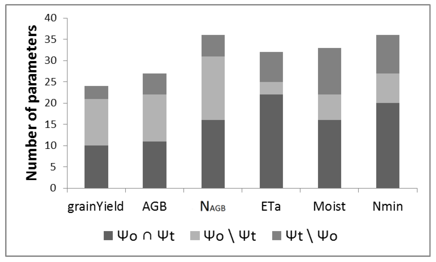
Applying both approaches, our objective was to identify all model parameters that were highly influential at some during simulation time. Choosing τ o = 0.2 for the original approach, we could identify all model parameters that affected the output at some point during simulation time. With a τ t = 0.8 for the extended approach, only parameters were selected that were highly influential at some point during simulation time. When analyzing Ψ o and Ψ t , we found that the numbers of identified parameters were comparable, and the majority of the identified model parameters were identified by both approaches (Figure 3). However, some parameters were identified by the new approach ( Ψ t ) that were not identified by the original approach, whereas some parameters were also found to be relevant using the original approach that were not included in Ψ t .
Table 3 lists the model parameters identified with τ t = 0.8 as calculated using the time-dependent Morris approach for all analyzed model outputs. Including the results of different study sites, a parameter was marked as relevant if at any site μ * was higher then the threshold value τ t . It shows that each model output is affected by a different set of model parameters. By comparing the results obtained using the extended approach for each study site, we found that each site was affected by different model parameters, whereas the identified parameters differed both in their number and composition. For example, the number (n) of relevant parameters for AGB differed. For Ascha and Guelzow, n = 8 parameters were selected, for Dornburg n = 10 , and for Ettlingen and Werlte, n = 12 . The parameter m a x A s s i m R a t e was sensitive for all sites, but m i n A v a i l a b l e N affected AGB only in Ascha, Ettlingen, or Werlte. However, because the screening method was only used as a preliminary means of identifying the most relevant model parameters for each output, we did not further analyze the differences among the sites using these screening results; instead, as described in Section 3.2.4, this comparison was performed using the more reliable sensitivity measures calculated using the time-dependent extended FAST method.

3.2. Extended FAST Method

3.2.1. Original Approach

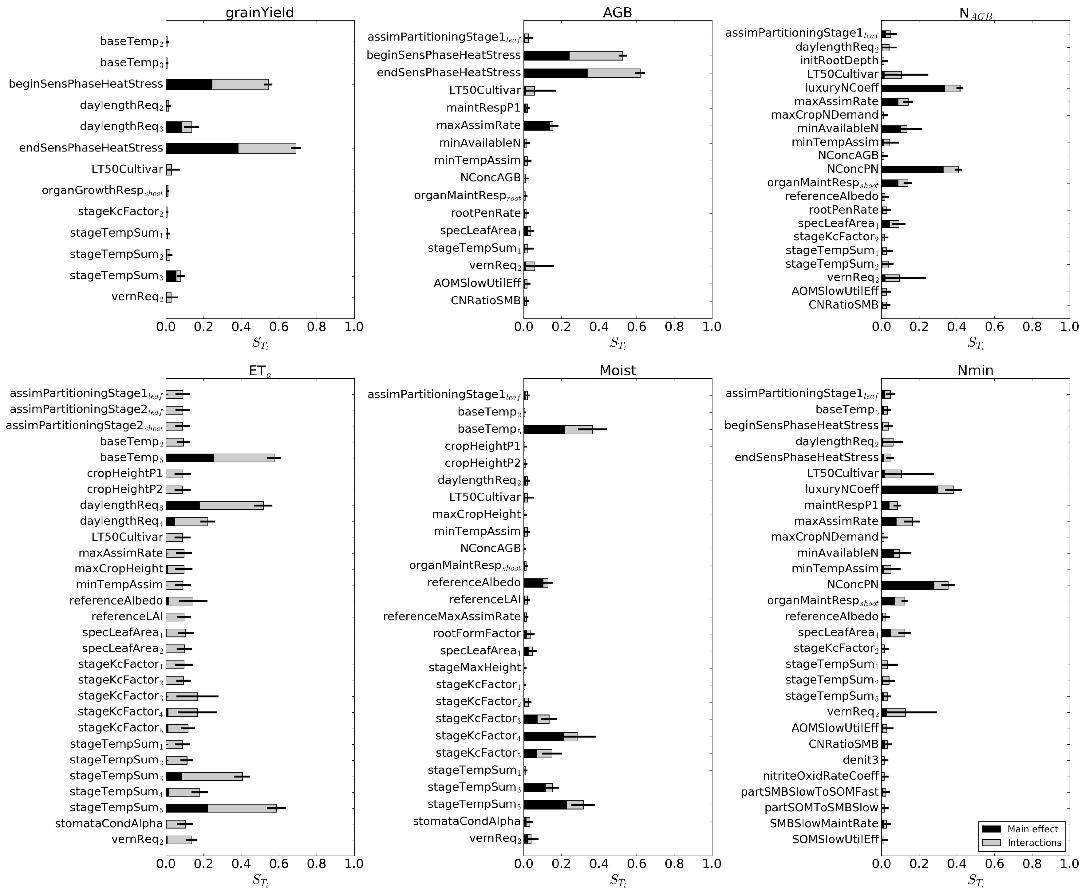
After identifying the most relevant model parameters based on the results of the extended screening method, we calculated the first-order ( S i ) and total ( S T i ) sensitivity indices using the extended FAST approach. The computation of both first-order and total sensitivity indices allows one to distinguish between main and interaction effects. The resulting estimates for the S T i averaged over all sites are shown in Figure 4.
The parameter sensitivity differed slightly among the analyzed sites. For Dornburg, the main variations in grainYield and AGB were caused by different sensitivity indices. For the heat stress parameters, the S T i and S i values were slightly lower compared with those at the other locations, where both sensitivity indices were quite similar. For Dornburg, the sensitivity indices for daylengthReq 3 , LT50Cultivar, stageTempSum 2 , stageTempSum 3 , and vernReq 2 were higher compared with the other sites. Similar results were found for N A G B and N m i n , for which parameters related to the crop phenology were associated with considerably higher sensitivities in Dornburg compared with the other locations. Analyzing the parameter sensitivity indices for ET a at the different locations revealed that although the orders of the parameters based on the sensitivity measures were the same, Ettlingen had the highest S T i and S i values, followed by Gülzow and Werlte. The parameter sensitivities for Moist also differed among the analyzed sites, but no generally applicable order of the important parameters based on S T i and S i was identified in this case.

3.2.2. Time-Dependent Main Effects

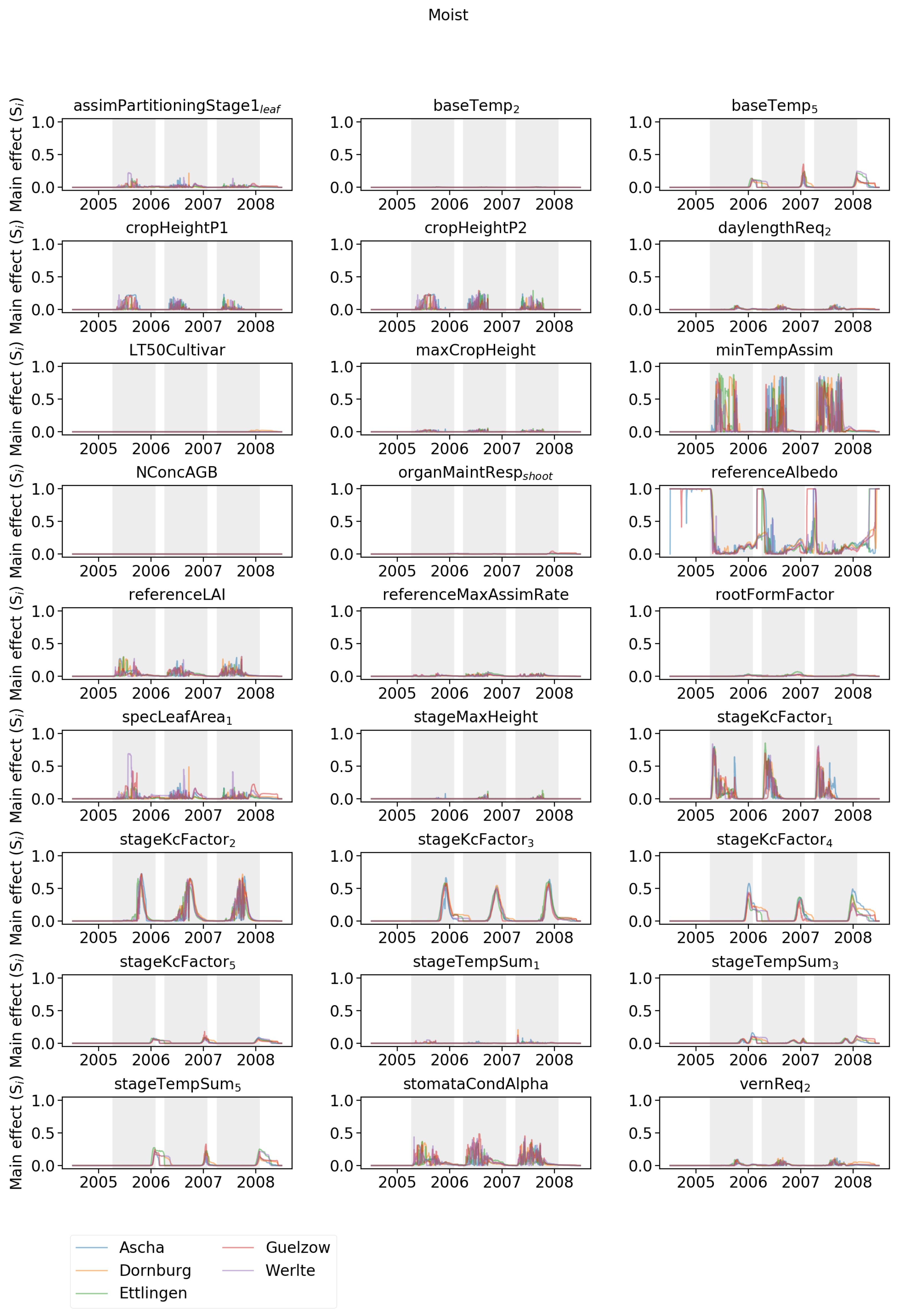
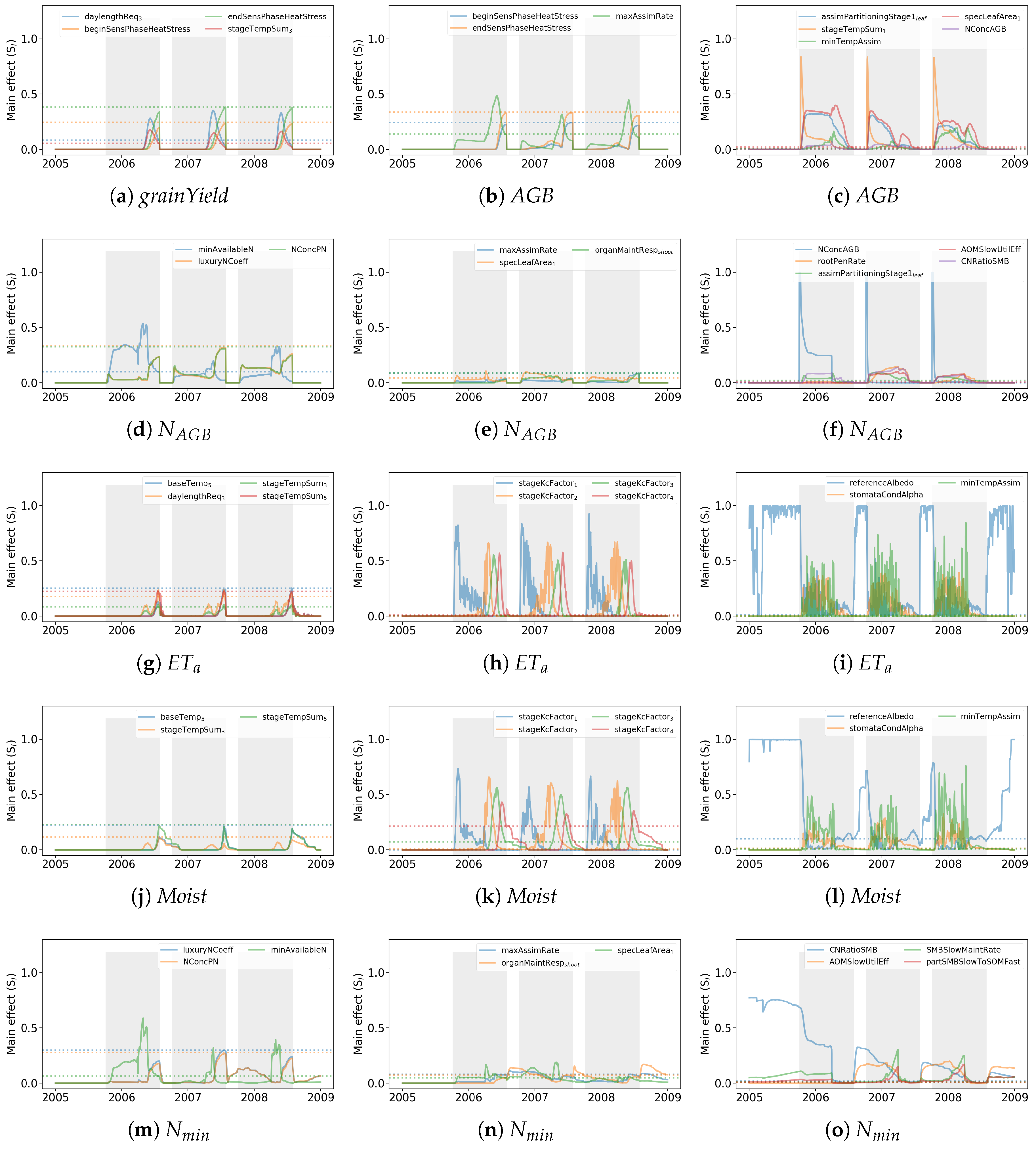
In addition to applying the original approach, we calculated the main effects of the model parameters for each time step of the simulation. Figure 5 displays the results of the temporal sensitivity analysis aggregated over all sites for a selection of the relevant model parameters. A complete overview of the calculated daily main effects for each analyzed parameter differentiated among the different sites is provided in the Appendix A in Figure A1, Figure A2, Figure A3, Figure A4, Figure A5 and Figure A6.
For biomass-related outputs such as grainYield, AGB, and N A G B , the time-dependent extended FAST method identified more sensitive parameters compared with the original approach. The temporal analysis of the main effects enabled the identification of not only parameters that were relevant at harvest time, but also ones that were relevant during earlier stages of crop development. assimPartitioningStage1 l e a f and specLeafArea 1 strongly affected AGB at the beginning of crop growth, but their influence decreased strongly over time until harvest. For N A G B , the influence of NConcAGB was very high during the first stage of development, but decreased once the flowering stage began.
Similar results were found for the soil-related outputs ET a , Moist and N m i n , for which the temporal sensitivity analysis enabled the detection of parameters that were influential at various times throughout the simulation, in contrast to the original approach, which analyzed the parameter sensitivities at only a single point in time. For ET a and Moist, the sensitivities to the crop’s transpiration parameters stageKcFactor 1 stageKcFactor 4 were very high in their respective developmental stages, but decreased as harvest time approached.

3.2.3. Temporal Sensitivity Patterns

For each simulation day, we generated a parameter ranking based on the daily main effects. We used the TDCCs to compare the parameter rankings for different simulation days averaged over all sites (Figure 6). For all crop-specific outputs (grainYield, AGB, and N A G B ), we compared the parameter sensitivity rankings solely for the cultivation period, because these outputs were not calculated for the fallow time. grainYield was calculated only for the last three developmental stages of the winter wheat. For this short period, we found an annual pattern of similar parameter sensitivities in which the sensitivities were more comparable at the beginning of this period and then decreased. For AGB, regardless of the simulation year, the agreement among parameter rankings was higher in earlier developmental stages at all sites. With the onset of the flowering phase, the differences in the parameter rankings increased. This general pattern could be found in every study site. However, analyzing the TDCC of AGB for each study site (Figure 7) showed that there are some periods where this pattern was only weakly pronounced. In Ettlingen, for example, the parameter ranking of 2006 and 2007 during spring differed highly. This indicates that due to differences in the site-specific climate conditions of both years, the parameter sensitivity for AGB differed. 2007 was characterized by a long spring drought with no precipitation compared to a relative wet spring in 2006. For N A G B , we found few agreements between parameter rankings for the early developmental stages in a single simulation year. For a short period at the end of crop growth, the parameter rankings for the different simulation years were quite similar. Analyzing the TDCC of N A G B showed less concordance for 2007 compared to the other years; again, presumably due to the exceptional weather conditions in 2007.
Fewer seasonal patterns were found for the soil-specific model output. We identified a small annual pattern of similar parameter sensitivities for ET a and Moist, especially at the beginning of crop growth, but also during further crop development. This means that sensitivity ranking did not differ for these periods. Comparing these time periods with the temporal main effects in Figure 5j–l, we found that E T a and M o i s t were mostly affected by the parameters s t a g e K c F a c t o r 1 s t a g e K c F a c t o r 4 regardless of the analyzed study site. For both outputs, the TDCC showed high consistency in parameter ranking in the early simulation days ending with the sowing of the crop. However, the TDCC also showed that the parameter sensitivity of the first growing season beginning with sowing in October 2005 differed strongly compared to the following growing seasons. Only a few agreements between the parameter sensitivities for different simulation days were found for N m i n . Regardless of the simulation year, a high TDCC was found for a short period directly before crop harvest. In this period, N m i n was mainly affected by parameters l u x u r y N C o e f f and N C o n c P N . Additionally, the TDCC for N m i n showed that the parameter rankings during crop growth for the last two cultivation periods were more similar than those for the first cultivation period.

3.2.4. Influence of the Different Sites

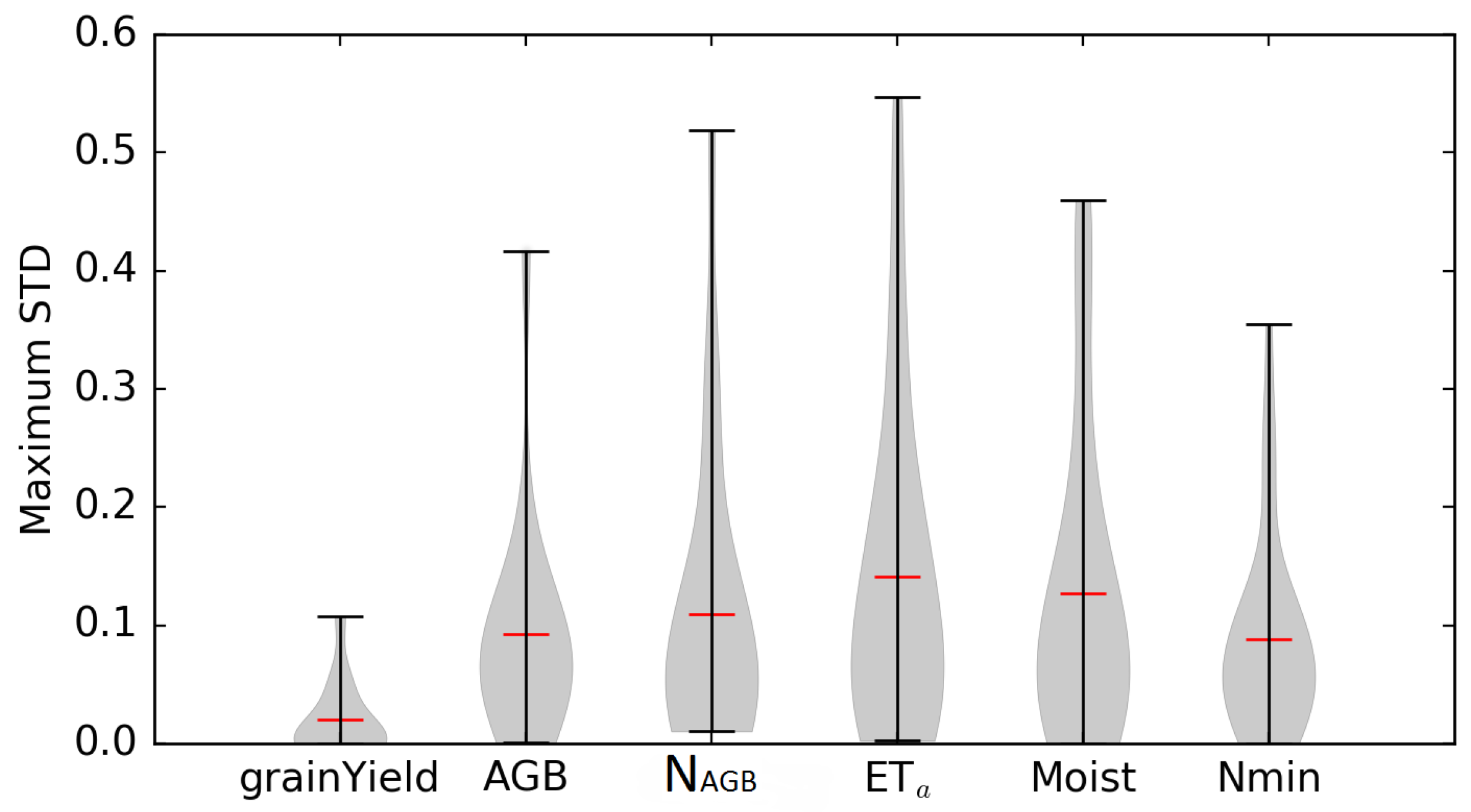
Regardless of the selected output, the parameter sensitivities differed among the analyzed sites (see Figure 8 and Figure A1, Figure A2, Figure A3, Figure A4, Figure A5 and Figure A6 in the Appendix A). Only minor differences in parameter sensitivity were found for grainYield. Site-specific differences for AGB were caused mainly by the parameters assimPartitioningStage1 l e a f , maxAssimRate, specLeafArea 1 , and minTempAssim. For N A G B , the variations were caused by NConcAGB and minAvailableN, especially during the first cultivation period. Regardless of the cultivation period, the parameter sensitivities of the remaining relevant parameters consistently differed among the different sites. Substantial variations in the sensitivities to several parameters were found for ET a , Moist, and N m i n , originating from site-specific differences in the most influential parameters.

4. Discussion

The previously-performed SA of the MONICA model [12] increased the understanding of the model and served as input for a later model calibration, but it yielded only a static snapshot of the parameter sensitivity at harvest time. The time-dependent SA presented in this study provides a deeper understanding of the model behavior and more detailed information about the influence of the model parameters throughout the simulation time. Many studies have used snapshot SAs to obtain general information on model behavior [12,15,16,33,39,45,46,47,48]; however, only a few studies have addressed the fact that parameter sensitivity is a function of time, and changes throughout the simulation time [18,19,33,49,50,51]. Ref. [20,21] present an alternative approach to account for the dynamics for parameter sensitivity complementing the approach applied in this study. This study, however, is the first to analyze the effect of the simulation time on the parameter sensitivity based on elementary effects calculated using the Morris screening design. The general approach used in this study can be easily applied for time-dependent SAs of other ecological models.
The results of the original and adopted Morris approaches strongly depend on the chosen threshold values τ o and τ t that are used to identify the relevant model parameters. When the threshold value is lower, a greater number of relevant model parameters are identified. We compared the identified parameters in Ψ o with the parameters in Ψ t . We used a low τ o to exclude parameters with negligible influence from Ψ o , respectively identify influential parameters. For Ψ t , we chose a high threshold value τ t = 0.8 to identify model parameters that had a significant influence at any point during the simulation time. With all outputs considered, the numbers of parameters in both sets were comparable, but not identical. The majority of parameters were identified in both sets, but some parameters were found to be relevant using one approach, but negligible according to the other approach. Similarly to [12,18,19,45,52], we used the Morris approach to screen out less influential parameters. The selection of a high threshold value allowed us to identify model parameters that had a strong effect at some point during the simulation time. Because the results of the original approach represent the aggregated parameter sensitivity based on a single point in time, we found the set of parameters identified using the temporal extension for the objective of this study to be more reliable and used the parameters in Ψ t for further temporal sensitivity analysis.
The original extended FAST method provides a measure of the sensitivity at only a single point throughout the simulation time, in our case at the harvesting of the winter wheat. The daily analysis of the main effects performed in this study showed that more parameters than those identified by the original approach affected the selected model outputs. With the new approach, we were also able to analyze the relationships between parameter sensitivity and crop growth using daily sensitivity values. Several parameters were highly influential during the early stages of crop development, but the corresponding parameter sensitivities declined during crop growth. For example, stageTempSum 1 had a minor effect on AGB (S i = 0.0) according to the original approach. However, upon analyzing the parameter sensitivity using the daily main effect values, we found that this parameter had a major impact on AGB during the initial stages of crop development (S i > 0.8 ) and then steadily decreased in influence until harvest time. Similar observations apply to other parameters (specLeafArea 1 for AGB, NConcAGB for N A G B , stageKcFactor 1 for Moist), whose associated sensitivities decreased during crop development or with increasing simulation time. Additionally, we identified parameters that had no effect at the beginning of crop growth, but whose influence increased during crop development, e.g., endSensPhaseHeatStress for grainYield and NConcPN for N A G B or N m i n . Other parameters showed a peak-shaped sensitivity evolution; the model’s sensitivity to these parameters was low during early stages of crop growth, then increased to a maximum, and finally steadily decreased once again as the simulation progressed further (stageKcFactor 1 stageKcFactor 4 for ET a or Moist). referenceAlbedo was the only parameter that had a major effect during fallow time, but only a minor influence on ET a and Moist during crop growth.
Often, SA at a single simulation time is used to identify relevant model parameters that are later used for model calibration [12,53]. The time-dependent SA results presented here demonstrate that such snapshot SAs may lead to incorrect interpretations of the parameters’ influences. Calibration studies relying on snapshot SAs may be insufficient and lack the necessary information on how the parameter sensitivity changes over the simulation time. Additionally, the analyses of parameter sensitivities for different sites indicate the strong influence of soil and climate conditions on parameter sensitivity [18,19]. A temporal sensitivity analysis can improve the calibration process for a model, depending on the scope of the calibration and the data available to be used for calibration. Temporal sensitivity analysis enables the identification of influential parameters for different simulation periods. A crop model calibration can benefit from such results if measured data regarding the model outputs are available for different times throughout the model simulation. Then, a set of parameters that are specific to a certain simulation time for which measured data exist can be selectively adopted to improve the results of the model calibration. If experimental data are available for only one specific time, then a snapshot sensitivity analysis should be sufficient for model calibration.
The TDCCs based on the parameter rankings for different simulation days revealed some temporal patterns of similarity in parameter sensitivities. For each output, we found an annual pattern of similar parameter sensitivities for some phase of crop development, although the climate conditions differed for each cultivation year. For the crop-specific model outputs, more pronounced seasonal sensitivity patterns could be identified, which means that the calculated parameter rankings were similar for longer simulation periods, as well as for different simulation years. Such a pattern could be expected as some relevant model parameters are only active during a specific developmental stage. Parameter rankings for soil-related model outputs such as Moist or N m i n were less homogeneous and were more affected by site-specific conditions of different simulation years. Similar parameter rankings were only identified for small simulation periods during crop development caused by the high influence of only a few parameters for this period. However, the temporal TDCCs also demonstrated the site-specific effect of soil and climate conditions on the parameter sensitivity, as the parameter rankings from one year differed highly compared to the other simulation years.
Differences in the soil and climate conditions also affected the parameter sensitivities [13,15,18], as indicated by the fact that the values and shapes of the sensitivity results differed for the different analyzed study sites. ET a and Moist showed the highest differences in parameter sensitivity. Because both of these outputs strongly rely on the water storage capacity of the soil and the available water (precipitation and capillary rise from groundwater), both are highly sensitive to different site and climate conditions. N A G B and N m i n were affected by a similar set of parameters (e.g., minAvailableN, luxuryNCoeff, NConcPN), although the form of the relationship differed slightly. The parameter sensitivities for the different analyzed sites differed greatly, especially with regard to the most influential parameters. Both outputs depend on the available nitrogen (N) stored in the soil, which is influenced by the soil type at the site. Additionally, mineralization processes of the soil microbial biomass (SMB) that transform added organic matter (e.g., crop residues or organic fertilizer) into plant-available nitrogen are highly dependent on temperature. Both of these factors contributed to the site-specific differences we detected in the parameters to which N A G B and N m i n were sensitive. Because the simulation time over which grainYield was calculated was rather short, only minor site-specific differences were identified in this output.
The temporal sensitivity analysis in this study was based on the calculation of first-order sensitivity indices. We used main effects (1) for analyzing the course of sensitivity during simulation time and (2) for generating the parameters’ ranking on which the calculation of TDCCs was based. As Figure 4 shows, the interaction effects of parameters are quite high. In this study, we deliberately focused on the main effects to quantify the direct effect of model parameters on the output. Using the total effect would not deliver any information on the direct contribution of the model parameters or on the contribution of the interaction with other parameters. For a sound interpretation of total effects, it is still necessary to know the main effect of model parameters.
In this study, we deliberately focused on the main effects to quantify the direct effect of model parameters towards the output. By using the total effect, there would be a high uncertainty for how much this influence was caused directly by the model parameters or how much it was caused by the interaction with other parameters. For a correct interpretation of the total effects, it is still necessary to know the main effect of the model parameters.
In this study, SA was performed at five different sites to demonstrate the influence of different soil and climate conditions on parameter sensitivity. We focused on the general effects of the different sites on the time-dependent SA results. Consequently, this study lacks a detailed analysis of how the parameter sensitivity is affected by single driving variables (e.g., soil texture, air temperature, precipitation). Future SA studies performed to further improve the understanding of the model behavior should consider both the temporal dynamics of parameter sensitivity and the effects of different sites and climate conditions. Such a study using a more comprehensive SA scheme should therefore concentrate on the specific effects of individual driving variables on the time-dependent parameter sensitivity.

5. Conclusions

The temporal dynamics of parameter sensitivity and the use of site-specific data will typically hamper a comprehensive sensitivity analysis of an (agro-)ecological model. Our comparison of the original and time-dependent screening approaches revealed that the original approach, which aggregates the parameter sensitivity over a certain simulation time, will fail to identify parameters to which the model is highly sensitive for only a limited period during the simulation. The time-dependent screening approach permits more reliable identification of the relevant model parameters, which helps to yield a better understanding of the behavior of process-based models and to better assist in their improvement. It is evident that calibration studies in which SA is applied to identify relevant model parameters must include an analysis of the temporal dynamics of parameter sensitivity; otherwise, the results of a snapshot SA may lead to incorrect interpretations of the parameters’ influences.
Most process-based agro-ecosystem models include processes that are only active during a certain period of the simulation, and consequently, their parameters are similarly only relevant during a certain period. A model calibration can benefit from a temporal SA because it enables a detailed identification of the influential model parameters that acknowledges their limited temporal activity. Unlike a snapshot SA, a temporal SA also permits the analysis of the relationships between model parameters and outputs, which supports a more thorough understanding and evaluation of model behavior. This is particularly important for understanding the influence of site conditions on the simulation and considering parameter estimation with respect to a particular environment. A temporal SA may provide hints regarding how to prioritize the experimental observations of crucially sensitive parameters to improve the general logic of the experiment-algorithm-simulation model-prediction chain.
Although it still seems challenging to quantify the influence of site conditions to obtain a more objective interpretation of parameter sensitivity, this study already serves as a step toward reducing the uncertainty of model simulations conducted with limited available data, as demonstrated by [54] for the improvement of a model algorithm that had previously been identified in a variable-focused SA as being a source of disagreement between models [55].

Author Contributions

X.S.: conceptualization, methodology, software, analysis, writing, original draft preparation, visualization; C.N.: conceptualization, writing, review and editing, supervision; R.W.: writing, review and editing, supervision.

Funding

This research was funded by the German Federal Ministry of Food and Agriculture and the Agency for Renewable Resources as part of the research project “Development and comparison of optimized cropping systems for the agricultural production of energy crops”, Grant Number FKZ 22013008.

Conflicts of Interest

The authors declare no conflict of interest. The funders had no role in the design of the study; in the collection, analyses, or interpretation of data; in the writing of the manuscript; nor in the decision to publish the results.

Abbreviations

The following abbreviations are used in this manuscript:
AGBAbove-ground biomass
C o r g Organic carbon
CANCalcium-ammonium-nitrate-based fertilizer
EEElementary effect
ET 0 Potential evapotranspiration
ET a Actual evapotranspiration
FASTFourier amplitude sensitivity test
HPCHigh-performance computer
MoistSoil moisture
MONICAModel for Nitrogen and Carbon dynamics in Agro-ecosystems
N A G B N content in above-ground biomass
N m i n Soil mineral nitrogen
SASensitivity analysis
S i First-order sensitivity index
S T i Total sensitivity index
TDCCTop-down concordance coefficients
TDSATime-dependent sensitivity analysis

Software availability

Name of SoftwareMONICA—Model for Nitrogen and Carbon dynamics in Agro-ecosystems
Version1.2
DeveloperClaas Nendel
ContactClaas Nendel, Leibniz Centre for Agricultural Landscape Research (ZALF), Research Platform ’Models’, Eberswalder Straße 84, 15374 Müncheberg, Germany
Email: [email protected] Tel.: +49-33432 82-355 Fax: +49-33432-82-181
Year first available2011
Required hardware and softwareMONICA will run on Windows or Linux machines. When building the model directly from the source code MONICA requires Boost.Python Version 1.0. For Windows systems the compilation process requires Visual Studio 2015 (Community Edition).
Availability and CostInformation about the MONICA model can be found at http://monica.agrosystem-models.com. For Windows an installation wizard can be downloaded at http://monica.agrosystem-models.com. The source code of the model is available at Github (https://github.com/zalf-rpm/monica).
Cost and LicenseFree. MONICA is distributed under the Mozilla Public License, v.2.0 (http://mozilla.org/MPL/2.0/)
Program LanguageMONICA was developed using the programming language C/C++. Model parameters are stored in a separate SQLite database that comes with the model.
Program sizeSource code: approx. 20 MB
Windows installer: 2.6 MB

Appendix A. Daily Parameter Sensitivities Based on SI Differentiated among the Different Sites

In this section, the main effects calculated for each site based on the extended FAST method are presented.
Figure A1. Daily S i values calculated using the extended FAST method for grainYield differentiated among the different sites.
Agriculture 09 00037 g0a1
Figure A2. Daily S i values calculated using the extended FAST method for AGB differentiated among the different sites.
Agriculture 09 00037 g0a2
Figure A3. Daily S i values calculated using the extended FAST method for N A G B differentiated among the different sites.
Agriculture 09 00037 g0a3
Figure A4. Daily S i values calculated using the extended FAST method for ET a differentiated among the different sites.
Agriculture 09 00037 g0a4
Figure A5. Daily S i values calculated using the extended FAST method for Moist differentiated among the different sites.
Agriculture 09 00037 g0a5
Figure A6. Daily S i values calculated using the extended FAST method for N m i n differentiated among the different sites.
Agriculture 09 00037 g0a6

References

  1. Martre, P.; Wallach, D.; Asseng, S.; Ewert, F.; Jones, J.W.; Rötter, R.P.; Boote, K.J.; Ruane, A.C.; Thorburn, P.J.; Cammarano, D.; et al. Multimodel ensembles of wheat growth: Many models are better than one. Glob. Chang. Biol. 2015, 21, 911–925. [Google Scholar] [CrossRef] [PubMed]
  2. Asseng, S.; Ewert, F.; Martre, P.; Roetter, R.P.; Lobell, D.B.; Cammarano, D.; Kimball, B.A.; Ottman, M.J.; Wall, G.W.; White, J.W.; et al. Rising temperatures reduce global wheat production. Nat. Clim. Chang. 2015, 5, 143–147. [Google Scholar] [CrossRef]
  3. Bassu, S.; Brisson, N.; Durand, J.L.; Boote, K.; Lizaso, J.; Jones, J.W.; Rosenzweig, C.; Ruane, A.C.; Adam, M.; Baron, C.; et al. How do various maize crop models vary in their responses to climate change factors? Glob. Chang. Biol. 2014, 20, 2301–2320. [Google Scholar] [CrossRef] [PubMed] [Green Version]
  4. Ewert, F.; Rötter, R.; Bindi, M.; Webber, H.; Trnka, M.; Kersebaum, K.; Olesen, J.; van Ittersum, M.; Janssen, S.; Rivington, M.; et al. Crop modelling for integrated assessment of risk to food production from climate change. Environ. Model. Softw. 2014. [Google Scholar] [CrossRef]
  5. Makowski, D.; Naud, C.; Jeuffroy, M.H.; Barbottin, A.; Monod, H. Global sensitivity analysis for calculating the contribution of genetic parameters to the variance of crop model prediction. Reliab. Eng. Syst. Saf. 2006, 91, 1142–1147. [Google Scholar] [CrossRef]
  6. Mirzaei, M.; Huang, Y.F.; El-Shafie, A.; Shatirah, A. Application of the generalized likelihood uncertainty estimation (GLUE) approach for assessing uncertainty in hydrological models: A review. Stoch. Environ. Res. Risk Assess. 2015, 29, 1265–1273. [Google Scholar] [CrossRef]
  7. Uniyal, B.; Jha, M.K.; Verma, A.K. Parameter identification and uncertainty analysis for simulating streamflow in a river basin of Eastern India. Hydrol. Process. 2015, 29, 3744–3766. [Google Scholar] [CrossRef]
  8. Ma, S.; Churkina, G.; Wieland, R.; Gessler, A. Optimization and evaluation of the ANTHRO-BGC model for winter crops in Europe. Ecol. Model. 2011, 222, 3662–3679. [Google Scholar] [CrossRef]
  9. Muleta, M.; Nicklow, J. Sensitivity and uncertainty analysis coupled with automatic calibration for a distributed watershed model. J. Hydrol. 2005, 306, 127–145. [Google Scholar] [CrossRef]
  10. Confalonieri, R.; Bregaglio, S.; Acutis, M. Quantifying plasticity in simulation models. Ecol. Model. 2012, 225, 159–166. [Google Scholar] [CrossRef]
  11. Jakeman, A.; Letcher, R.; Norton, J. Ten iterative steps in development and evaluation of environmental models. Environ. Model. Softw. 2006, 21, 602–614. [Google Scholar] [CrossRef]
  12. Specka, X.; Nendel, C.; Wieland, R. Analyzing the parameter sensitivity of the agro-ecosystem model MONICA for different crops. Eur. J. Agron. 2015, 71, 73–87. [Google Scholar] [CrossRef]
  13. Richter, G.M.; Acutis, M.; Trevisiol, P.; Latiri, K.; Confalonieri, R. Sensitivity analysis for a complex crop model applied to Durum wheat in the Mediterranean. Eur. J. Agron. 2010, 32, 127–136. [Google Scholar] [CrossRef]
  14. Saltelli, A.; Chan, K.; Scott, E.M. Sensitivity Analysis; John Wiliey & Sons, Ltd.: Hoboken, NJ, USA, 2000. [Google Scholar]
  15. Dzotsi, K.; Basso, B.; Jones, J. Development, uncertainty and sensitivity analysis of the simple SALUS crop model in DSSAT. Ecol. Model. 2013, 260, 62–76. [Google Scholar] [CrossRef]
  16. Makler-Pick, V.; Gal, G.; Gorfine, M.; Hipsey, M.R.; Carmel, Y. Sensitivity analysis for complex ecological models—A new approach. Environ. Model. Softw. 2011, 26, 124–134. [Google Scholar] [CrossRef]
  17. Zhao, G.; Bryan, B.; Song, X. Sensitivity and uncertainty analysis of the APSIM-wheat model: Interactions between cultivar, environmental, and management parameters. Ecol. Model. 2014, 279, 1–11. [Google Scholar] [CrossRef]
  18. Song, X.; Bryan, B.; Almeida, A.; Paul, K.; Zhao, G.; Ren, Y. Time-dependent sensitivity of a process-based ecological model. Ecol. Model. 2013, 265, 114–123. [Google Scholar] [CrossRef]
  19. Song, X.; Bryan, B.; Paul, K.; Zhao, G. Variance-based sensitivity analysis of a forest growth model. Ecol. Model. 2012, 247, 135–143. [Google Scholar] [CrossRef]
  20. Lamboni, M.; Monod, H.; Makowski, D. Multivariate sensitivity analysis to measure global contribution of input factors in dynamic models. Reliab. Eng. Syst. Saf. 2011, 96, 450–459. [Google Scholar] [CrossRef]
  21. Lamboni, M.; Makowski, D.; Lehuger, S.; Gabrielle, B.; Monod, H. Multivariate global sensitivity analysis for dynamic crop models. Field Crops Res. 2009, 113, 312–320. [Google Scholar] [CrossRef]
  22. Nendel, C.; Berg, M.; Kersebaum, K.; Mirschel, W.; Specka, X.; Wegehenkel, M.; Wenkel, K.; Wieland, R. The MONICA model: Testing predictability for crop growth, soil moisture and nitrogen dynamics. Ecol. Model. 2011, 222, 1614–1625. [Google Scholar] [CrossRef]
  23. Kersebaum, K. Application of a simple management model to simulate water and nitrogen dynamics. Ecol. Model. 1995, 81, 145–156. [Google Scholar] [CrossRef]
  24. Greenwood, D.; Stone, D.; Draycott, A. Weather, nitrogen-supply and growth rate of field vegetables. Plant Soil 1990, 124, 297–301. [Google Scholar] [CrossRef]
  25. Wegehenkel, M. Test of a modelling system for simulating water balances and plant growth using various different complex approaches. Ecol. Model. 2000, 129, 39–64. [Google Scholar] [CrossRef]
  26. Allen, R.G.; Pereira, L.S.; Raes, D.; Smith, M. Crop Evapotranspiration. Guidelines for Computing Crop Water Requirements; FAO Irrigation and Drainage Paper; FAO: Roma, Italy, 1998; Volume 56. [Google Scholar]
  27. Hansen, S.; Jensen, H.; Nielsen, N.; Svendsen, H. Simulation of nitrogen dynamics and biomass production in winter wheat using the Danish simulation model DAISY. Fertili. Res. 1991, 27, 245–259. [Google Scholar] [CrossRef]
  28. Glemnitz, M.; Eckner, J.; Aurbacher, J.; Kornatz, P.; Müller, J.; Heiermann, M.; Peter, C. Crop rotations as “cornerstone” of sustainable energy cropping—Integrative evaluation of their agronomic, ecologic, economic and resource efficiency effects. In Biomass and Energy Crops V; Association of Applied Biologists: Brussels, Belgium, 2015; pp. 117–128. [Google Scholar]
  29. Nehring, A.; Vetter, A. Entwicklung und Vergleich von Optimierten Anbausystemen für die landwirtschaftliche Produktion von Energiepflanzen unter den Verschiedenen Standortbeding ungen Deutschlands (EVA)—Abschlussbericht 2009 zum Teilprojekt 1; Technical Report; Thüringer Landesanstalt für Landwirtschaft: Jena, Germany, 2009.
  30. Vetter, A.; Nehring, A.; Ebel, G.; Peters, J.; Grunewald, J.; Kruse, S.; Deiglmayr, K.; Wilken, F. Schriftliche Mitteilung. Datenmaterial aus den Bonituren des deutschlandweiten Verbundprojektes EVA; Technical Report; Thüringer Landesanstalt für Landwirtschaft: Jena, Germany, 2011; FKZ 22013008.
  31. Esprey, L.; Sands, P.; Smith, C. Understanding 3-PG using a sensitivity analysis. For. Ecol. Manag. 2004, 193, 235–250. [Google Scholar] [CrossRef]
  32. Morris, M.D. Factorial Sampling Plans for Preliminary Computational Experiments. Technometrics 1991, 33, 161–174. [Google Scholar] [CrossRef] [Green Version]
  33. Campolongo, F.; Cariboni, J.; Saltelli, A. An effective screening design for sensitivity analysis of large models. Environ. Model. Softw. 2007, 22, 1509–1518. [Google Scholar] [CrossRef]
  34. Sin, G.; Gernaey, K.V. Improving the Morris method for sensitivity analysis by scaling the elementary effects. In 19th European Symposium on Computer Aided Process Engineering; Jezowski, J., Thullie, J., Eds.; Computer Aided Chemical Engineering; Elsevier: Amsterdam, The Netherlands, 2009; Volume 26, pp. 925–930. [Google Scholar]
  35. Saltelli, A.; Tarantola, S.; Chan, K.P.S. A quantitative model-independent method for global sensitivity analysis of model output. Technometrics 1999, 41, 39–56. [Google Scholar] [CrossRef]
  36. Cukier, R.I.; Fortuin, C.M.; Shuler, K.E.; Petschek, A.G.; Schaibly, J.H. Study of the sensitivity of coupled reaction systems to uncertainties in rate coefficients. I Theory. J. Chem. Phys. 1973, 59, 3873–3878. [Google Scholar] [CrossRef]
  37. Iman, R.L.; Conover, W. A measure of top-down correlation. Technometrics 1987, 29, 351–357. [Google Scholar]
  38. Helton, J.; Johnson, J.; Sallaberry, C.; Storlie, C. Survey of sampling-based methods for uncertainty and sensitivity analysis. Reliab. Eng. Syst. Saf. 2006, 91, 1175–1209. [Google Scholar] [CrossRef] [Green Version]
  39. Confalonieri, R.; Bellocchi, G.; Bregaglio, S.; Donatelli, M.; Acutis, M. Comparison of sensitivity analysis techniques: A case study with the rice model WARM. Ecol. Model. 2010, 221, 1897–1906. [Google Scholar] [CrossRef]
  40. Savage, I. Contributions to the theory of rank order statistics—The two-sample case. Ann. Math. Stat. 1956, 27, 590–615. [Google Scholar] [CrossRef]
  41. Lutz, M. Programming Python, 4th ed.; O’Reilly: Sebastopol, CA, USA, 2010. [Google Scholar]
  42. Beazley, D. Automated scientific software scripting with SWIG. Future Gener. Comput. Syst. 2003, 19, 599–609. [Google Scholar] [CrossRef]
  43. Dalcín, L.; Paz, R.; Storti, M. MPI for Python. J. Parallel Distrib. Comput. 2005, 65, 1108–1115. [Google Scholar] [CrossRef]
  44. Dalcín, L.; Paz, R.; Storti, M.; D’Elía, J. MPI for Python: Performance improvements and MPI-2 extensions. J. Parallel Distrib. Comput. 2008, 68, 655–662. [Google Scholar] [CrossRef]
  45. Confalonieri, R.; Bellocchi, G.; Tarantola, S.; Acutis, M.; Donatelli, M.; Genovese, G. Sensitivity analysis of the rice model WARM in Europe: Exploring the effects of different locations, climates and methods of analysis on model sensitivity to crop parameters. Environ. Model. Softw. 2010, 25, 479–488. [Google Scholar] [CrossRef] [Green Version]
  46. Estrada, V.; Diaz, M. Global sensitivity analysis in the development of first principle-based eutrophication models. Environ. Model. Softw. 2010, 25, 1539–1551. [Google Scholar] [CrossRef]
  47. Francos, A.; Elorza, F.J.; Bouraoui, F.; Bidoglio, G.; Galbiati, L. Sensitivity analysis of distributed environmental simulation models: understanding the model behavior in hydrological studies at the catchment scale. Reliab. Eng. Syst. Saf. 2003, 79, 205–218. [Google Scholar] [CrossRef]
  48. Campolongo, F.; Saltelli, A. Sensitivity analysis of an environmental model an application of different analysis methods. Reliab. Eng. Syst. Saf. 1997, 57, 49–69. [Google Scholar] [CrossRef]
  49. Simons-Legaard, E.; Legaard, K.; Weiskittel, A. Predicting aboveground biomass with LANDIS-II: A global and temporal analysis of parameter sensitivity. Ecol. Model. 2015, 313, 325–332. [Google Scholar] [CrossRef] [Green Version]
  50. Garambois, P.A.; Roux, H.; Larnier, K.; Castaings, W.; Dartus, D. Characterization of process-oriented hydrologic model behavior with temporal sensitivity analysis for flash floods in Mediterranean catchments. Hydrol. Earth Syst. Sci. 2013, 17, 2305–2322. [Google Scholar] [CrossRef] [Green Version]
  51. Reusser, D.E.; Buytaert, W.; Zehe, E. Temporal dynamics of model parameter sensitivity for computationally expensive models with the Fourier amplitude sensitivity test. Water Resour. Res. 2011, 47, W07551. [Google Scholar] [CrossRef]
  52. Saltelli, A.; Annoni, P. How to avoid a perfunctory sensitivity analysis. Environ. Model. Softw. 2010, 25, 1508–1517. [Google Scholar] [CrossRef]
  53. Wallach, D.; Makowski, D.; Jones, J.W. (Eds.) Working with Dynamic Crop Modells; Elsevier: Amsterdam, The Netherlands, 2006. [Google Scholar]
  54. Wang, E.; Martre, P.; Asseng, S.; Ewert, F.; Zhao, Z.; Maiorano, A.; Rötter, R.; Kimball, B.; Ottman, M.; Wall, G.; et al. Generic temperature response functions reduce uncertainty in crop yield projections. Nat. Plants 2016. in revision. [Google Scholar]
  55. Asseng, S.; Ewert, F.; Rosenzweig, C.; Jones, J.W.; Hatfield, J.L.; Ruane, A.C.; Boote, K.J.; Thorburn, P.J.; Rotter, R.P.; Cammarano, D.; et al. Uncertainty in simulating wheat yields under climate change. Nat. Clim. Chang. 2013, 3, 827–832. [Google Scholar] [CrossRef]
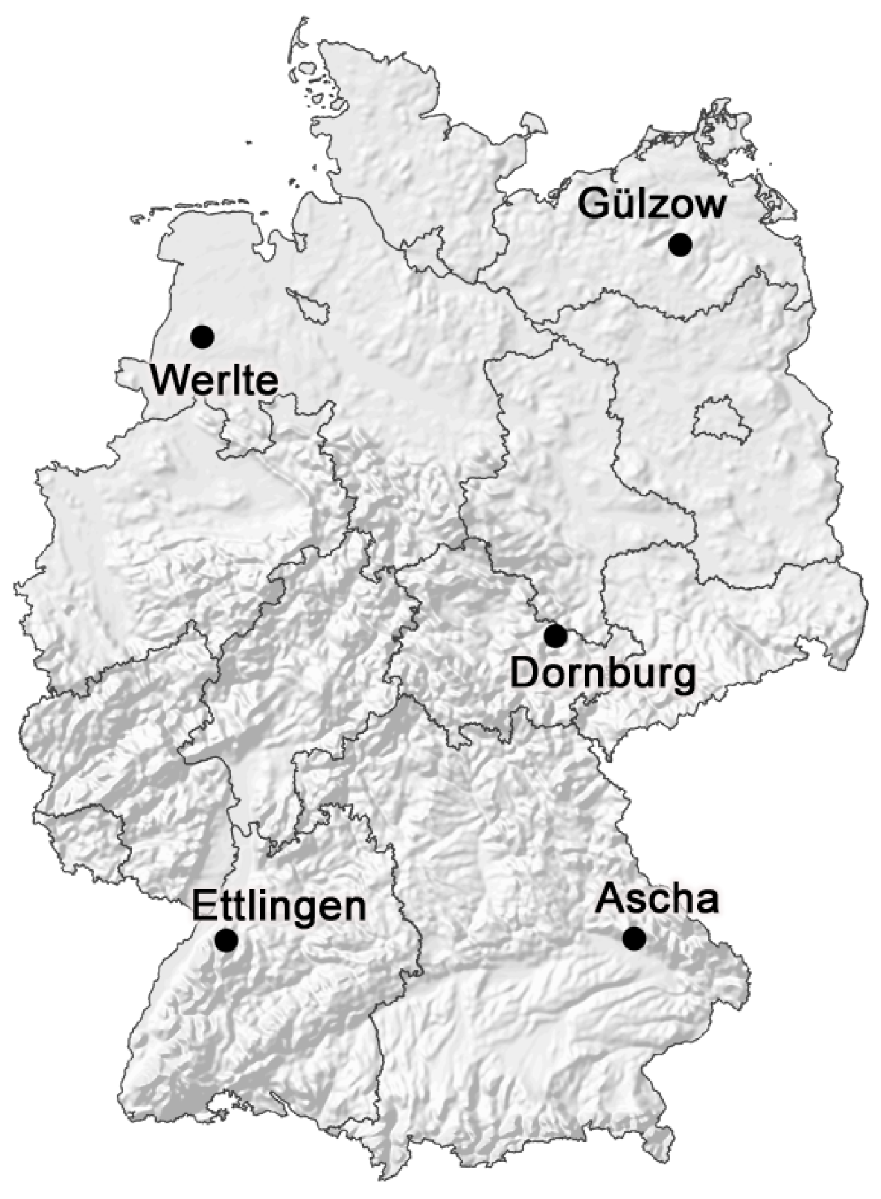
Figure 1. Locations of the five study sites in Germany. Detailed information and descriptions of the site characteristics can be found in Table 1.
Agriculture 09 00037 g001
Figure 2. Numbers of relevant parameters identified by the original (dark gray) and extended (light gray) Morris methods as functions of the threshold values τ o and τ t , respectively, for the example of AGB. A parameter was marked as relevant if at any study site μ * was higher than the respective threshold value.
Agriculture 09 00037 g002
Figure 3. Numbers of relevant parameters identified by the original and extended Morris methods using τ o = 0.2 and τ t = 0.8 , respectively. Ψ o Ψ t denotes the model parameters that exist in both sets. Ψ o \ Ψ t denotes the model parameters that are included in Ψ o , but not in Ψ t . Ψ t \ Ψ o denotes the parameters that are included in Ψ t , but not in Ψ o .
Agriculture 09 00037 g003
Figure 4. Total sensitivity indices for the most relevant model parameters calculated using the extended FAST approach averaged over all sites. The main effect denotes the portion of the total variance that is explained by the given parameter. The interactions represent the portion that is explained by all parameter interactions involving that parameter. The sum of the main effect and the interactions corresponds to the total sensitivity index ( S T i ) of the parameter.
Agriculture 09 00037 g004
Figure 5. Variations in parameter sensitivities with simulation time for various outputs averaged over all study sites. The solid lines indicate the time-dependent parameter sensitivities based on the main effects (S i ). The dotted lines represent the sensitivity values calculated based on the main effect indicated by the original extended FAST approach at harvest time (Figure 4). The gray shaded ranges correspond to the cultivation period for winter wheat, from sowing in October up through harvest in July (Table 2). Further information can be found in Figure A1, Figure A2, Figure A3, Figure A4, Figure A5 and Figure A6 in the Appendix A, which show in detail the time-dependent main effects differentiated for each study site.
Agriculture 09 00037 g005
Figure 6. TDCCs of parameter rankings based on the daily main effects for different simulation days, averaged over all study sties. A higher TDCC indicates greater similarity of the parameter rankings. The dark areas indicate periods during which the parameter rankings were similar for different simulation times.
Agriculture 09 00037 g006
Figure 7. TDCCs of parameter rankings for AGB based on the daily main effects for different simulation days differentiated for each study site. A higher TDCC indicates greater similarity of the parameter rankings. The dark areas indicate periods during which the parameter rankings were similar for different simulation times.
Agriculture 09 00037 g007
Figure 8. Variations in the main effects caused by site-specific differences in soil or weather conditions. The violin plots aggregate the maximum standard deviations of the daily S i values for all sites and each analyzed parameter.
Agriculture 09 00037 g008
Table 1. Characteristics of the experimental sites. Soil type is specified according to the FAO classification system. C o r g refers to the first 30 cm of the top soil layer. Total annual precipitation and mean temperature are averaged between 1971 and 2000.
NameAschaDornburgEttlingenGülzowWerlte
Geographical location 48 59 ′ N 50 48 ′ N 48 50 ′ N 53 42 ′ N 52 51 ′ N
12 65 ′ E 11 35 ′ E 8 41 ′ E 12 54 ′ E 7 41 ′ E
Height above sea level430 m250 m170 m10 m32 m
Soil typeStagnic CambisolLuvisolRegosol-LuvisolPlanosolStagnic Cambisol
Soil textureLoamy sandSilty clayey loamLoamy siltSandy loamLoamy sand
Available water capacity117 mm189–215 mm199 mm120 mm105 mm
C o r g 1.3%1.0%0.76%0.7%1.3%
pH value6.47.27.36.45.2
Total annual precipitation807 mm474 mm742 mm559 mm797 mm
Mean temperature7.5 C8.8 C11.1 C8.4 C9.57 C
Table 2. Artificial crop management setting used for the sensitivity analysis, in which CAN was used as a calcium-ammonium-nitrate-based nitrogen fertilizer. The management steps were repeated for each cultivation year, starting in 2005. The dates of the management steps were made consistent for each study site to facilitate the analysis of the temporal SA results.
PloughingSowingFertilizationHarvesting
3 October4 October31 March70 kg NCAN29 July
30 April30 kg NCAN
22 May60 kg NCAN
Table 3. Relevant model parameters as identified using the time-dependent Morris approach with τ t = 0.8 . A parameter was marked as relevant if its μ * ( t ) was higher than the threshold value τ t in one of the investigated sites.
ParameterDescriptionUnitNominalgrainYieldAGBN AGB ET a MoistN min
AOMSlowUtilEffAdded organic matter slow utilization efficiency 0.4 xx x
assimPartitioningStage1 l e a f Portion of assimilates assigned for leaf growth in Stage 1%0.5 xxxxx
assimPartitioningStage2 l e a f Portion of assimilates assigned for leaf growth in Stage 2%0.2 x
assimPartitioningStage2 s h o o t Portion of assimilates assigned for shoot growth in Stage 2%0.6 x
baseTemp 2 Base temperature for assimilation in Stage 2 C1x xx
baseTemp 3 Base temperature for assimilation in stage 3 C1x
baseTemp 5 Base temperature for assimilation in Stage 5 C9 xxx
beginSensPhaseHeatStressTemperature sum marking the start of the sensitive phase for heat stress C620xx x
CNRatioSMBC-to-N ratio of the soil microbial biomass6.7 xx x
cropHeightP1Factor for crop height6 xx
cropHeightP2Reduction factor for crop height0.5 xx
daylengthReq 2 Day length required for maximum growth in Stage 2h20x x xx
daylengthReq 3 Day length required for maximum growth in stage 3h20x x
daylengthReq 4 Day length required for maximum growth in Stage 4h20 x
denit3Denitrification coefficient 0.9 x
endSensPhaseHeatStressTemperature sum marking the end of the sensitive phase for heat stress C740xx x
initRootingDepthInitial root depth of the cropm0.1 x
LT50CultivarThreshold temperature below which 50% of the crop dies from frost injury C−24xxxxxx
luxuryNCoeffCoefficient describing the maximum N concentration relative to the critical N concentration in the crop tissue1.3 x x
maintRespP1Q 10 factor for maintenance respiration0.08 x x
maxAssimRateMaximum assimilation rate per leaf areakg CO 2 ha 1 52 xxx x
maxCropHeightMaximum crop heightm0.83 xx
maxCropNDemandMaximum amount of soil mineral N to be taken up by the crop kg m 2 6 x x
minAvailableNMineral N concentration in the soil that is not available for crop N uptake kg m 3 0.0008 xx x
minTempAssimMinimum temperature required for assimilation C4 xxxxx
NConcAGBDefault N concentration in above-ground biomasskg kg 1 0.06 xx x
nConcPNShape factor for the critical N curve1.6 x x
nitrRateCoeffStandNitrification rate default coefficientd 1 0.2 x
organMaintResp s h o o t Maintenance respiration factor for shootskg CO 2 kg DM 1 0.15xxx xx
partSMBSlowToSOMFastPortion of the soil microbial biomass that is added to the fast soil organic matter pool 0.6 x
partSOMToSMBSlowPortion of the soil organic matter that is added to the slow soil microbial biomass pool 0.015 x
referenceAlbedoFAO reference albedo for green grass0.23 xxxx
referenceLAILeaf area index of the reference cropm 2 kg 1 1.44 xx
referenceMaxAssimRateMaximum assimilation rate of the reference cropkg CO 2 4 ha 1 30 x
rootFormFactorFactor describing the root mass distribution pattern with respect to depth3 x
rootPenRateVertical root growth ratem C 1 d 1 0.0011 xx
SMBSlowMaintRateStandMaintenance rate for slowly-reproducing soil microbial biomassd 1 0.001 x
SOMSlowUtilEffMicrobial utilization efficiency for the slowly-decomposing soil organic matter pool 0.4 x
specificLeafArea 1 Specific leaf area for calculating the leaf area index for stage 1m 2 kg 1 0.002 xxxxx
specificLeafArea 2 Specific leaf area for calculating the leaf area index for stage 2m 2 kg 1 0.0018 x
stageAtMaxHeightStage of maximal crop height3 x
stageKcFactor 1 K c factor for Stage 10.4 xx
stageKcFactor 2 K c factor for Stage 20.7x xxxx
stageKcFactor 3 K c factor for Stage 31.1 xx
stageKcFactor 4 K c factor for stage 41.1 xx
stageKcFactor 5 K c factor for Stage 50.8 xx
stageTempSum 1 Temperature sum for Stage 1 C148xxxxxx
stageTempSum 2 Temperature sum for Stage 2 C284x xx x
stageTempSum 3 Temperature sum for Stage 3 C380x xx
stageTempSum 4 Temperature sum for Stage 4 C180 x
stageTempSum 5 Temperature sum for Stage 5 C420 xxx
stomataCondAlphaStomata conductivity parameter40 xx
vernReq 2 Temperature sum required for optimum vernalization in Stage 2 C50xxxxxx
Number of relevant parameters131621292729