Methods for Fitting the Limit State Function of the Residual Strength of Damaged Ships

Abstract

The limit state function is important for the assessment of the longitudinal strength of damaged ships under combined bending moments in severe waves. As the limit state function cannot be obtained directly, the common approach is to calculate the results for the residual strength and approximate the limit state function by fitting, for which various methods have been proposed. In this study, four commonly used fitting methods are investigated: namely, the least-squares method, the moving least-squares method, the radial basis function neural network method, and the weighted piecewise fitting method. These fitting methods are adopted to fit the limit state functions of four typically sample distribution models as well as a damaged tanker and damaged bulk carrier. The residual strength of a damaged ship is obtained by an improved Smith method that accounts for the rotation of the neutral axis. Analysis of the results shows the accuracy of the linear least-squares method and nonlinear least-squares method, which are most commonly used by researchers, is relatively poor, while the weighted piecewise fitting method is the better choice for all investigated combined-bending conditions.

1. Introduction

Ship safety is a major concern to researchers, and the number of damaged ships in accidents has been decreasing with advances in technology. According to the statistics of the International Association of Dry Cargo Shipowners, the loss of bulk carriers over 10,000 DWT has decreased from more than 500 in 1994–2003 to 202 in 2008–2017, and the number of casualties has also decreased from more than 200 to 53. In order to further reduce the casualties and property losses, researchers have continued their effort on the improvement of ship safety. When the ship is subjected to collision and grounding, which are the major types of accidents [1], the longitudinal strength will decrease and the wave load will change as well. Owing to the damage-induced change in floating state of the damaged ship, the wave load behavior is more complicated than the intact ship. Chen et al. [2] investigated the wave load of a damaged RO-RO ship and found the horizontal load is as large as 1.73 times the vertical load in the oblique wave. The ultimate-strength assessment method is well established for the vertical load on intact ships [3] but not for damaged ships. Therefore, it is necessary to devise a method for the damaged ship under combined bending moments. For this purpose, the limit state function is key to the method.

The longitudinal-strength assessment method for intact ships can be calculated directly by the Smith method and the Finite Element Method (FEM). There are more studies about the ultimate strength based on these methods [4,5,6,7,8]. However, it is difficult to directly obtain the longitudinal strength of the ship under combined bending moments, and one has to rely on the limit state function for the assessment of ship safety. The accuracy of the limit state function depends on the ultimate-strength calculation method and the fitting method. To obtain accurate samples for the fitting of the limit state function, a variety of methods have been proposed. Yao et al. [9] applied a simplified progressive collapse method to study the longitudinal strength of the bulk carrier under bi-axis bending moments. Parunov et al. [10] investigated the longitudinal strength of a damaged tanker under combined bending moments with the FEM, and the relationship between the damage size and the longitudinal strength was discussed. Paik et al. [11,12] compared the longitudinal strength of unstiffened and stiffened plates under combined loads. Dow et al. [13] explored the longitudinal strength of a stiffened box girder under combined bending moments with the Smith method and the FEM. Paik et al. [14] studied corroded stiffened plates under combined compression loads with the FEM. Fujikubo et al. [15] investigated the longitudinal strength of the stiffened plate under the combined shear and thrust force with the FEM. Dow et al. [16] studied the longitudinal strength of an alloy plate under combined shear and compression/tension with the FEM. Among the methods widely used in the community, the FEM can account for the initial implication, the material nonlinearity and the geometric nonlinearity. The finite element models provide more details about the structures, and the relationship between adjacent parts is taken into account. However, the method costs much more time for modeling and computation. The Smith method only needs to discretize a cross section into stiffened plate elements, plate elements, and hard-corner elements. As the curvature increases, the stress and the bending moment of each element are calculated according to the strain–stress relationship curves of different element types, and the sum of the element bending moment is the bending moment of the cross section. This method is much more efficient, but the accuracy is poor when applied to ships with asymmetric cross sections. To improve the accuracy of the method in nonsymmetric applications, improved Smith methods were devised by Fujikubo et al. [17] and Joonmo et al. [18]. Fujikubo et al. [17] applied an improved Smith method to damaged ships, and proposed an equation to describe the relationship between the increments of vertical and horizontal bending moments and the increments of the curvatures. Joonmo et al. [19] proposed the force vector equilibrium criterion to track the rotation of the neutral axis so as to obtain the bending moments of the asymmetric cross section.

Once samples of longitudinal strength are obtained, the limit state function can be approximated by means of fitting. Gordo et al. [19,20] applied a nonlinear fitting method to obtain the limit state function of the longitudinal strength of a tanker under combined bending moments. Monsour et al. [21] applied a nonlinear fitting method to obtain the limit state functions of different ships. Luis et al. [22] adopted a nonlinear fitting method to fit the limit state functions of two damaged tankers. Khan et al. [23] also used a nonlinear fitting method to fit the limit state functions and explored the reliabilities of a damaged tanker and a bulk carrier. Shahid [24] used the response surface method and the artificial neural network to fit the limit state function. Zhu et al. [25] proposed the weighted piecewise fitting method for the limit state function. Paik et al. [26] investigated the longitudinal strength of the as-built ultra-large containership under combined vertical bending and torsion, then fitted the limit state function with a nonlinear method and obtained the design load area. Kim et al. [27] studied the longitudinal strength of the hull girder under combined bending and torsion and obtained a ¼ circular form of the limit state function by fitting. Shi et al. [28] compared the longitudinal strength of open box girders with cracked damage under pure vertical bending load and combined loads, and a circular form of the limit state function was also obtained by fitting. Hu et al. [29] studied the longitudinal strength of a large opening box girder with a crack under torsion and bending loads and presented the interaction between the two loads in a circular form. The same form of the limit state function was also used by Li et al. [30], who investigated the pipe under combined bending and torsion moment. Though the fitting methods are used in many research studies, the accuracy and the applicability of the fitting methods remain unclear and need to be studied.

As the ship structure and damage condition can be different from one another, the limit state curves may also be different from one another, but all of them are closed curves in the coordinate system. In the existing studies, four typical closed curves are adopted to approximate the curve: (1) circle, (2) transverse ellipse, (3) vertical ellipse, and (4) oblique ellipse. Four fitting methods are proposed and investigated in this study: namely, (1) the least-squares method, (2) the moving least-squares method (MLS), (3) the radial basis artificial neural network method (RBFNN), and (4) the weighted piecewise fitting method (WP). Finally, samples of longitudinal strength for a damaged tanker and damaged bulk carrier calculated by Fujikubo et al. [12] were obtained for the fitting method study.

2. Fitting Methods for the Limit State Function

2.1. The Least-Squares Method

The least-squares method adopts the linear or nonlinear regression to establish a polynomial function. The general form of the linear polynomial function is $a+b=c$:

$$\overline{Y}=C_0+{\displaystyle \sum _{i=1}^n{C}_i{X}_i}+{\displaystyle \sum _{i=1}^n{\displaystyle \sum _{j=1}^n{C}_{ij}{X}_i}}{X}_j+\epsilon ,$$

(1)

where $\overline{Y}$ is the regression result of the fitting function for the $n$ random variables $X_i$, $C$ is the regression coefficient, and $\epsilon$ is the error between the regression result and the actual response.

Quadratic functions and cubic functions are commonly used linear least-squares fitting functions. They take the following forms, respectively:

$$y=a+bx+c{x}^2,$$

(2)

$$y=a+bx+c{x}^2+d{x}^3$$

(3)

where $x=M_H/M_{UH}$ and $y=M_V/M_{UV}$; where $M_V$ and $M_H$ are the vertical and horizontal bending moment, respectively, and $M_{UV}$ and $M_{UH}$ are the ultimate bending moments resulted from pure vertical and horizontal bending, respectively. In the case of multiple-valued functions, the following functions are used instead:

$$x=a+by+c{y}^2,$$

(4)

$$x=a+by+c{y}^2+d{y}^3,$$

(5)

Nonlinear functions are also widely used in least-squares fitting, where an often-used form is

$$x^{{\alpha }_1}+y^{{\alpha }_2}=1,$$

(6)

2.2. The Moving Least-Squares Method

Different from the classic polynomial function, the coefficient vectors of the moving least-squares-based fitting function and the basis functions are determined by the fitting results. The function usually takes the form

$$y={\displaystyle \sum _{i=1}^m{\alpha }_i(x)p_i(x)=p^{\mathrm{T}}(x)\alpha (x)},$$

(7)

where $p^{\mathrm{T}}(x)$ is the basis function, $\alpha (x)$ is the coefficient vector, m is the number of terms, and

$$p^{\mathrm{T}}(x)=[p_1(x),p_2(x),\cdots ,p_m(x)],$$

(8)

$${\alpha }^{\mathrm{T}}(x)=[{\alpha }_1(x),{\alpha }_2(x),\cdots ,{\alpha }_m(x)],$$

(9)

To extend the fitting range, the samples are described in polar coordinates, and the fitting function is

$$r=p^{\mathrm{T}}(\theta )\alpha (\theta ),$$

(10)

where r is the distance between the sample and the origin and $\theta$ is the angle between the point and the positive direction of the x-axis at the origin.

2.3. The Radial Basis Function Neural Network Method

The radial basis function is a function that relies only on the distance between the point x and the origin (or the calculation point c), which takes the form

$$\mathsf{\Phi }(x)=\mathsf{\Phi }(\Vert x\Vert ),$$

(11)

or

$$\mathsf{\Phi }(x,c)=\mathsf{\Phi }(\Vert x-c\Vert ),$$

(12)

where $\Vert x-c\Vert$ is the Euclidean distance between point x and point c.

The radial basis function neural network (RBFNN) is a neural network comprised of three layers: the input layer, the hidden layer, and the output layer, as shown in Figure 1. The RBF is the basis of the hidden layer. The transformation between the input layer and the hidden layer is nonlinear, while the transformation between the hidden and output layers is linear.

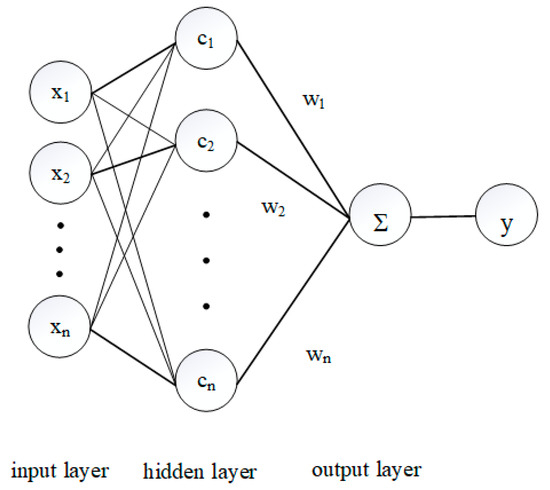
Figure 1. Typical form of the RBFNN.

The activation function is

$$\begin{array}{cc}\phi (x_k-c_i)=\exp (-\frac{1}{2{\sigma }^2}{\Vert x_k-c_i\Vert }^2)& (k=1,2,\dots ,l;i=1,2,\dots ,m\end{array}),$$

(13)

where $x_k$ is the k-th input data, $c_i$ is the center of the i-th neuron, and $\sigma$ is the standard deviation

$$\sigma =\frac{c_{\max }}{\sqrt{2h}},$$

(14)

where $h$ is the number of the centers that determines the K-means clustering and $c_{\max }$ is the maximum distance among the chosen centers.

The output of the neural network is

$$\begin{array}{cc}{y}_i={\displaystyle \sum _{i=1}^h{w}_{ij}\exp (-\frac{1}{2{\sigma }^2}{\Vert x_k-c_i\Vert }^2)}& (j=1,2,\dots ,n\end{array}),$$

(15)

where $w_{ij}$ is the weight of the i-th neuron for the output

$$w=\exp \left(\frac{h}{c_{\max }^2}{\Vert x_k-c_i\Vert }^2\right)(j=1,2,\dots ,n),$$

(16)

Once the RBFNN-based calculation is carried out, the input vector $X_{p\times 1}$ can be transformed into the output vector $Y_{n\times 1}$.

When the method is used to fit the samples in the polar coordinate system, the output of the neural network takes the form

$$\begin{array}{cc}{r}_i={\displaystyle \sum _{i=1}^h{w}_{ij}\exp (-\frac{1}{2{\sigma }^2}{\Vert {\theta }_k-c_i\Vert }^2)}& (j=1,2,\dots ,n\end{array}),$$

(17)

2.4. The Weighted Piecewise Fitting Method

The weighted piecewise fitting method provides a series of functions to describe the response relationship [20]. It adopts a piecewise regression method to fit the Function (3), and the weights matrix $w$ is introduced to improve the accuracy. With the sample matrix $X$ and $Y$, the coefficient matrix $N$ is

$$N={\left(X^{T}wX\right)}^{-1}{X}^{T}wY,$$

(18)

where

$$N={\left\{a,b,c,d\right\}}^T,$$

(19)

$$X=\left[\begin{array}{l}1\hspace{0.17em}{x}_1\hspace{0.17em}\hspace{0.17em}{x}_1{}^2\hspace{0.17em}{x}_1{}^3\\ 1\hspace{0.17em}{x}_2\hspace{0.17em}{x}_2{}^2\hspace{0.17em}{x}_2{}^3\\ ⋮\hspace{0.17em}\hspace{0.17em}\hspace{0.17em}⋮\hspace{0.17em}\hspace{0.17em}\hspace{0.17em}\hspace{0.17em}\hspace{0.17em}⋮\hspace{0.17em}\hspace{0.17em}\hspace{0.17em}\hspace{0.17em}\hspace{0.17em}\hspace{0.17em}⋮\\ 1\hspace{0.17em}{x}_m\hspace{0.17em}{x}_m{}^2\hspace{0.17em}{x}_m{}^3\end{array}\right],$$

(20)

$$Y={\left\{y_1,y_2,\dots ,y_m\right\}}^T,$$

(21)

where a, b, c, and d are the coefficients of the function. $x_i$ and $y_i$ is the i-th sample for the fitting.

Once the fitting functions for all samples are obtained, the values at both ends of each piece, $y_{i1}$ and $y_{i2}$, and the slopes ${y^{\prime }}_{i1}$ and ${y^{\prime }}_{i2}$ can be found. As the two adjacent piece functions must be smooth at the joint, the following boundary conditions are applied:

$$y_{i2}=y_{(i+1)1}=y_i,$$

(22)

$$\{\begin{array}{l}{y^{\prime }}_{i1}=({y^{\prime }}_{(i-1)2}+{y^{\prime }}_{i1})/2\\ {y^{\prime }}_{i2}=({y^{\prime }}_{i2}+{y^{\prime }}_{(i+1)1})/2\end{array},$$

(23)

In order to obtain a closed curve, the following boundary conditions are used:

$$\{\begin{array}{l}{y}_{(n+1)1}=y_1\\ {y^{\prime }}_{(n+1)1}={y^{\prime }}_{11}\end{array},$$

(24)

The coefficients of the fitting function of each piece need be recalculated with $y$ and $y^{\prime }$ at the curve ends as follows:

$$\{\begin{array}{l}{y}_{i1}=a_i+b_i{x}_{i1}+c_i{x}_{i1}^2+d_i{x}_{i1}^3\\ {y^{\prime }}_{i1}=b_i+2c_i{x}_{i1}+3d_i{x}_{i1}^2\\ y_{i2}=a_i+b_i{x}_{i2}+c_i{x}_{i2}^2+d_i{x}_{i2}^3\\ {y^{\prime }}_{i2}=b_i+2c_i{x}_{i2}+3d_i{x}_{i2}^2\end{array},$$

(25)

3. Calculation and Analysis of Typical Fitting Sample Distributions

In order to compare the difference between the fitting methods, six fitting methods are adopted to fit the function using typical fitting sample distributions: namely, the least-squares method with the quadratic function (LS-Q), the cubic function (LS-C), and the nonlinear function (LS-N); the moving least-squares method; the radial basis function neural network method; and the weighted piecewise fitting method.

3.1. Typical Fitting Sample Distribution

The distribution pattern of the sample of the longitudinal strength of the ship structures under combined bending moments is usually a closed curve, and the shape depends on the type and the damage of the structures. To present the representative conclusion, four typical distributions (TD1–TD4) are obtained for research after comparing the fitting sample distributions in the literature [15,16,17,18,19,20,21,22,23,24], as shown in Figure 2, where x and y represent the input data and output data of the fitting sample.

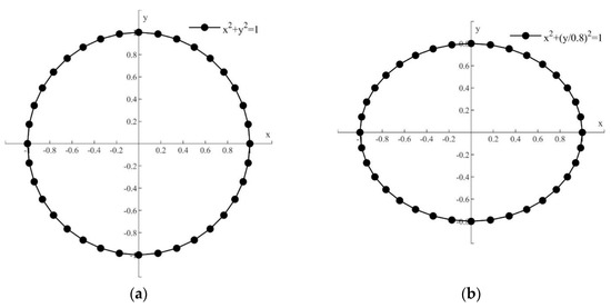
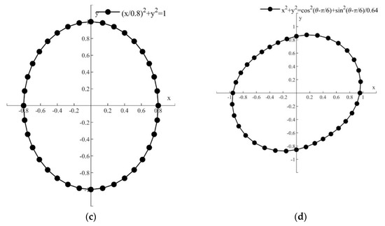
Figure 2. Fitting sample distributions for (a) TD1, (b) TD2, (c) TD3, and (d) TD4.

3.2. Fitting and Analysis of the Typical Distribution

The results obtained with the fitting methods for the typical distributions are shown in Figure 3.

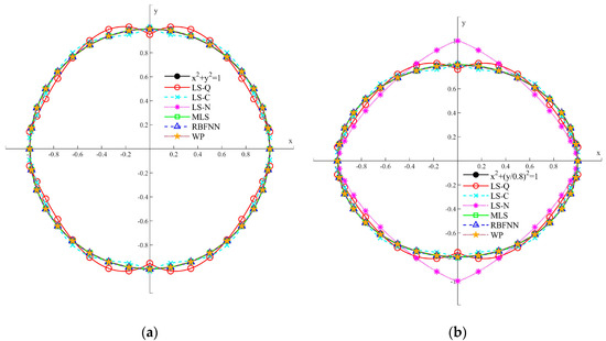
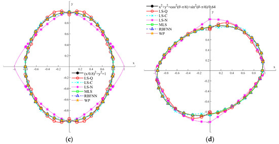
Figure 3. Fitting results for (a) TD1, (b) TD2, (c) TD3, and (d) TD4.

In order to compare the accuracy of the fitting methods, the y of the sample and the fitting results $y_{fitting}$ are shown in Figure 3, where the abscissa represents the $y$ of the sample and the ordinate denotes the fitted results $y_{fitting}$. The vertical distance between the fitting results for y and the line $y_{fitting}=y$ is the error of the fitting, and when the point is located on the line $y_{fitting}=y$, it means that the fitting result is accurate. Two types of fitting are performed: (1) Case 1, fitting for the sample data and (2) Case 2, fitting for the removed-sample data.

The maximum error and the mean square errors (MSE) of the fitting results of the sample data and the sample-removed data are calculated. The errors are shown in Table 1, Table 2, Table 3 and Table 4, and the MSE is

$$MSE=\frac{{\displaystyle \sum _{i=1}^n{\left(y_{fitting}-y\right)}^2}}{n},$$

(26)

Table 1. Maximum error and MSE for TD1.

Project	Case	LS-Q	LS-C	LS-N	MLS	RBFNN	WP
maximum error	Case 1	0.1427	0.0930	<1 × 10−4	<1 × 10−4	<1 × 10−4	0
	Case 2	0.0996	0.0823	<1 × 10−4	<1 × 10−4	<1 × 10−4	0.0081
MSE	Case 1	0.0043	0.0019	<1 × 10−8	<1 × 10−8	<1 × 10−8	0
	Case 2	0.0041	0.0024	<1 × 10−8	<1 × 10−8	<1 × 10−8	1.09 × 10−5

Table 2. Maximum error and MSE for TD2.

Project	Case	LS-Q	LS-C	LS-N	MLS	RBFNN	WP
maximum error	Case 1	0.1142	0.0744	0.2000	0.0008	<1 × 10−4	0
	Case 2	0.0796	0.0658	0.1582	0.0108	<1 × 10−4	0.0073
MSE	Case 1	0.0028	0.0012	0.0105	2.80 × 10−7	<1 × 10−8	0
	Case 2	0.0026	0.0016	0.0134	1.20 × 10−5	<1 × 10−8	7.71 × 10−6

Table 3. Maximum error and MSE for TD3.

Project	Case	LS-Q	LS-C	LS-N	MLS	RBFNN	WP
maximum error	Case 1	0.1427	0.0930	0.3566	0.0024	<1 × 10−4	01
	Case 2	0.0996	0.0823	0.2511	0.0097	0.0003	0.00181
MSE	Case 1	0.0043	0.0019	0.0197	1.23 × 10−6	<1 × 10−8	0
	Case 2	0.0041	0.0024	0.0161	1.34 × 10−5	<1 × 10−8	1.02 × 10−5

Table 4. Maximum error and MSE for TD4.

Project	Case	LS-Q	LS-C	LS-N	MLS	RBFNN	WP
maximum error	Case 1	0.2071	0.1732	0.1891	0.0016	<1 × 10−4	0
	Case 2	0.1389	0.1386	0.1330	0.0593	0.0611	0.0334
MSE	Case 1	0.0046	0.0028	0.0076	6.84 × 10−7	<1 × 10−8	0
	Case 2	0.0040	0.0029	0.0063	0.0002	0.0003	3.78 × 10−5

As shown in Figure 3, some fitting curves are not coincident with the sample curves, and the reason is that the shape and accuracy of the fitting curves depend on the sample distribution and the fitting method used. In Figure 4, it is found that the results calculated by the least-squares method have larger errors than others. The errors of LS-Q are larger than LS-C and LS-N when the sample distributions are TD1 and TD4. The errors of LS-N are larger than LS-Q and LS-C in TD2 and TD3. It is also observed in Table 1, Table 2, Table 3 and Table 4 that the maximum errors and MSE of LS-Q, LS-C, and LS-N are larger than that of MLS, RBFNN, and WP, and the error comparison between LS-Q, LS-C, and LS-N is the same as shown in Figure 4. The comparison between LS-Q and LS-C shows that increasing of the function order barely improves the fitting accuracy. The comparison of results obtained with LS-N shows the errors are larger when the sample is not −1 or 1 on the coordinate axis. It is also shown in Table 1, Table 2, Table 3 and Table 4 that the errors of LS-Q, LS-C, and LS-N in Case 1 are larger than in Case 2. The reason is that the least-squares method requires all data to obtain the minimum sum-of-squares errors. Therefore, the new sample for the fitting may change the fitting function and increase the fitting error. MLS, RBFNN, and WP need the sample near the fitting points, and the reduction of the sample may have a large influence on the fitting accuracy.

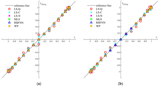
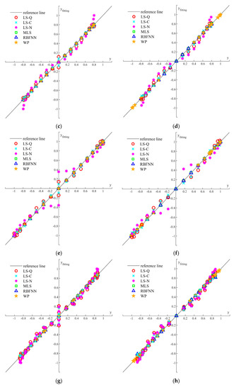
Figure 4. Accuracy comparison of fitting results for (a) TD1 in Case 1, (b) TD1 in Case 2, (c) TD2 in Case 1, (d) TD2 in Case 2, (e) TD3 in Case 1, (f) TD3 in Case 2, (g) TD4 in Case 1, and (h) TD4 in Case 2.

4. Calculation and Fitting for the Sample of the Damaged Ships

4.1. The Improved Smith Method

In the improved Smith method [17], the rotation of the neutral axis can be taken into account, which makes it applicable to asymmetric hull girder, for instance, damaged hull like the cross-section in Figure 5 under combined bending moments.

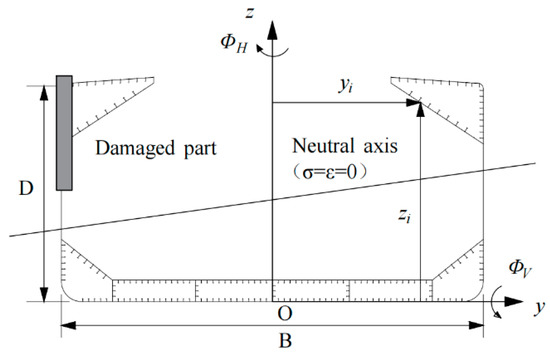
Figure 5. Cross section of a damaged ship.

The process for calculating the residual strength consists of 10 steps [3]:

(1)

The cross section of concern is divided into different types of stiffened plate units, plating units, and hard-corner units;

(2)

For a given curvature, the stress–strain relationships for all types of units are defined as shown in Figure 6. Then, the strain of the i-th unit is

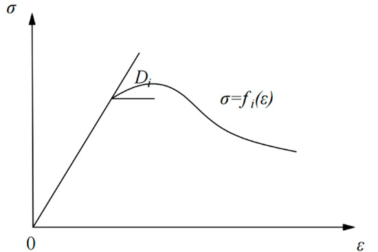Figure 6. Stress–strain curve.

$${\epsilon }_i(y_i,z_i)={\epsilon }_0+y_i{\mathsf{\Phi }}_H+z_i{\mathsf{\Phi }}_V,$$

(27)

where ${\epsilon }_0$ is the strain at the origin O and ${\mathsf{\Phi }}_H$ and ${\mathsf{\Phi }}_V$ are the horizontal curvature and vertical curvature, respectively. Then, the tangential stiffness $D_i$ can be calculated as

$$D_i=\frac{d{f}_i(\sigma )}{d\epsilon }=\frac{\Delta {\sigma }_i}{\Delta \epsilon },$$

(28)

(3)

The axial force P should satisfy

$$P={\displaystyle \sum _{i=1}^N{\sigma }_i{A}_i\equiv 0},$$

(29)

The vertical bending moment $M_V$ and the horizontal bending moment $M_H$ can be calculated as

$$\{\begin{array}{c}{M}_H={\displaystyle \sum _{i=1}^N{\sigma }_i{y}_i{A}_i}\\ M_V={\displaystyle \sum _{i=1}^N{\sigma }_i{z}_i{A}_i}\end{array},$$

(30)

where $A_i$ is the cross-sectional area of the i-th unit;

(4)

The position of point G is shown in Figure 7 and can be obtained by

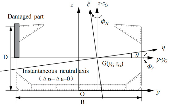Figure 7. Schemes follow the same formatting.

$$\{\begin{array}{c}{y}_G=\left({\displaystyle \sum _{i=1}^n{y}_i{D}_i{A}_i}\right)/\left({\displaystyle \sum _{i=1}^n{D}_i{A}_i}\right)\\ z_G=\left({\displaystyle \sum _{i=1}^n{z}_i{D}_i{A}_i}\right)/\left({\displaystyle \sum _{i=1}^n{D}_i{A}_i}\right)\end{array},$$

(31)

(5)

The flexural stiffness should satisfy the function

$$\left\{\begin{array}{c}\Delta M_H\\ \Delta M_V\end{array}\right\}=\left[\begin{array}{cc}{D}_{HH}& D_{HV}\\ D_{VH}& D_{VV}\end{array}\right]\left\{\begin{array}{c}\Delta {\mathsf{\Phi }}_H\\ \Delta {\mathsf{\Phi }}_V\end{array}\right\},$$

(32)

where

$$\{\begin{array}{c}{D}_{HH}={\displaystyle \sum _{i=1}^N{D}_i{(y_i-y_G)}^2{A}_i}\\ D_{VV}={\displaystyle \sum _{i=1}^N{D}_i{(z_i-z_G)}^2{A}_i}\\ D_{HV}=D_{VH}={\displaystyle \sum _{i=1}^N{D}_i(y_i-y_G)(z_i-z_G)A_i}\end{array},$$

(33)

(6)

The increments of the next curvature and/or bending moment can be calculated by

$$\left\{\begin{array}{c}\alpha \Delta M_H\\ \Delta M_V\end{array}\right\}=\left[\begin{array}{cc}{D}_{HH}& D_{HV}\\ D_{VH}& D_{VV}\end{array}\right]\left\{\begin{array}{c}\Delta {\mathsf{\Phi }}_H\\ \Delta {\mathsf{\Phi }}_V^0\end{array}\right\},$$

(34)

(7)

Increase the curvature, calculate the increment in strain and stress according to the stress–strain curve, and then the cumulative results of bending moment, strain, and stress of each unit can be obtained;

(8)

The position of the neutral axis can be calculated with the stress and strain

$${\epsilon }_0+y{\mathsf{\Phi }}_H+z{\mathsf{\Phi }}_V=0$$

(35)

(9)

When the ultimate strength is reached, the calculation is stopped.

4.2. Distribution of the Sample of Damaged Ships

In order to compare the accuracy of these fitting methods when applied to the limit state function, the sample of the longitudinal strength of a damaged single-hull bulk carrier (DB) and a damaged double-hull oil tanker (DT) calculated by Fujikubo et al. [17] are adopted. The main dimensions of the ships are shown in Table 5. The diagrammatic sketch of the cross sections and the damage conditions are shown in Figure 8.

Table 5. The main dimensions of the ships.

Ship Parameter	DB	DT
L (mm)	217,000	219,000
B (mm)	32,236	32,240
D (mm)	18,300	19,900

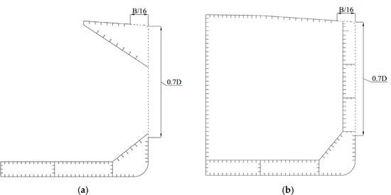
Figure 8. Cross sections of (a) DB and (b) DT.

The distribution of the results for the residual strength of DB and DT are shown in Figure 9.

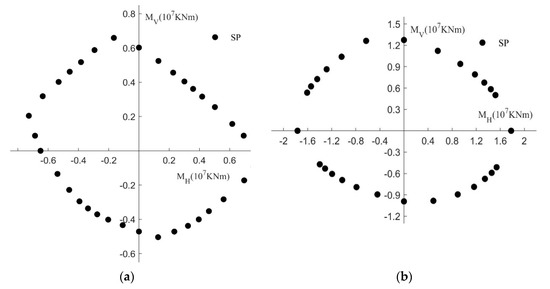
Figure 9. Distribution of sample for (a) DB and (b) DT.

4.3. Residual Strength Fitting Results for the Damaged Ships

The envelopes of bending moments of different ships or damaged cases are not different. In order to facilitate the comparison, the vertical bending moments and horizontal bending moments are nondimensionalized separately by the maximum vertical bending moment and the maximum vertical bending moment, respectively. The fitting results are shown in Figure 10. The fitting results of Case 1 and Case 2 are shown in Figure 11. The maximum errors and MSEs are shown in Table 6 and Table 7.

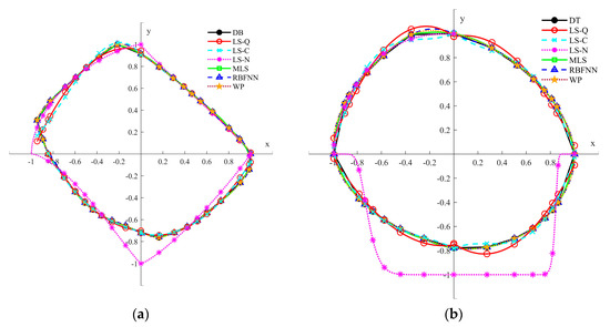
Figure 10. Fitting results for (a) DB and (b) DT.

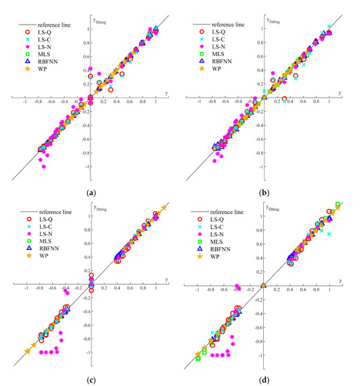
Figure 11. Accuracy comparison of fitting results for (a) DB in Case 1, (b) DB in Case 2, (c) DT in Case 1, and (d) DT in Case 2.

Table 6. Maximum error and MSE for TD1.

Project	Case	LS-Q	LS-C	LS-N	MLS	RBFNN	WP
maximum error	Case 1	0.3121	0.2944	0.4264	0.0129	0.0087	0.0000
	Case 2	0.3267	0.3640	0.2209	0.0471	0.0650	0.0404
MSE	Case 1	0.0046	0.0043	0.0138	8.53 × 10−6	8.21 × 10−6	0.0000
	Case 2	0.0054	0.0075	0.0072	0.0001	0.0005	0.0001

Table 7. Maximum error and MSE for TD2.

Project	Case	LS-Q	LS-C	LS-N	MLS	RBFNN	WP
maximum error	Case 1	0.1326	0.0740	0.4658	0.0024	0.0008	0.0000
	Case 2	0.1069	0.2451	0.4682	0.0700	0.0378	0.0750
MSE	Case 1	0.0026	0.0008	0.0419	1.30 × 10−6	1.66 × 10−7	0.0000
	Case 2	0.0035	0.0047	0.0576	0.0008	0.0001	0.0003

It is shown in Figure 10 that the deviation between fitting curves of LS-Q, LS-C, and LS-N and sample curves is larger than the curves of MLS, RBFNN, and WP. The fitting accuracy of LS-Q and LS-C is poor when the sample curves have more than one inflection point in a single quadrant, such as the curve in the second quadrant in Figure 10a, of which y increases and then decreases near $x=0$ and of which x decreases and then increases near $x=-1$. The fitting accuracy of LS-N is poor when the sample curves do not pass the points (1,0), (0,1), (−1,0), and (0,−1), such as the curve in the fourth quadrant in Figure 10b, which is flat, vertical, and then flat with decreasing x. It depends on the function of LS-N, and influences the curve shape and accuracy. The fitting curves of MLS, RBFNN, and WP are near the sample curves. In Figure 11, it can be found that when y is near −1, 0 and 1, $y_{fitting}$ of LS-Q, LS-C, and LS-N is usually far away from the reference line, which is disadvantageous for the assessment of the ship-hull girder residual strength under vertical bending moments. Comparison of Case 1 and Case 2 shows that the fitting accuracy of LS-Q, LS-C, and LS-N is also poor for the nonsample, and the fitting errors obviously increment or reduce. Comparing Case 1 of MLS for DT, the fitting errors of Case 2 increase when y is near 1 or −1, and the reason is that the lack of inflection point decreases the accuracy. The fitting accuracy of RBFNN and WP is high. In Table 6 and Table 7, it is shown that the maximum error and MSE of Case 1 and Case 2 of LS-Q, LS-C, and LS-N are large and close, but the maximum error and MSE of Case 2 of MLS, RBFNN, and WP are larger than in Case 1. The fitting results also show that LS-Q, LS-C, and LS-N can provide the explicit fitting functions in a single quadrant, and the fitting curves of LS-Q and LS-C are not continuous as well as LS-N not being smooth. The fitting curves of MLS, RBFNN, and WP are continuous and smooth, and a series of explicit fitting functions is obtained with WP, while the implicit fitting functions are obtained with MLS and RBFNN.

5. Conclusions

In this study, four fitting methods and six fitting functions are applied to calculate the fitting curves of four typical sample distributions and the longitudinal strength of two damaged ships under combined bending moments. Based on analysis of the results, the following conclusions are drawn:

(1)

The distribution of the sample influences the fitting accuracy. When the sample curves have multiple inflection points in a single quadrant and the curves do not pass the points (1,0), (0,1), (−1,0), and (0,−1), the difference between the fitting curves and the sample curves is large.

(2)

The least-squares method can fit the curves with different fitting functions and all the functions are explicit, but the fitting accuracies of the quadratic function, the cubic function, and the nonlinear function are not satisfactory. The fitting curves of the linear functions are not continuous, and the nonlinear functions are not smooth. The fitting results also show that the increase in the sample and the order of the function has little contribution to the fitting accuracy.

(3)

Application of MLS, RBFNN, and WP are more complex than the least-squares method, but the fitting accuracy is much better. All the fitting curves are continuous and smooth in the four quadrants, and they are able to improve the assessment accuracy of the residual strength under pure or combined bending moments. It can also be found that the increment of the sample has little contribution to the fitting accuracy.

(4)

The implicit fitting function can be obtained with MLS and RBFNN, and a series of explicit fitting functions can be obtained with WP.

References

- European Maritime Safety Agency (EMSA). Annual Overview of Marine Casualties and Incidents 2019; EMSA: Lisbon, Portugal, 2019. [Google Scholar]
- Chan, H.S.; Incecik, A.; Atlar, M. Structural Integrity of a Damaged Ro-Ro Vessel. In Proceedings of the Second International Conference on Collision and Grounding of Ships, Copenhagen, Denmark, 1–3 July 2001; Technical University of Denmark: Lyngby, Denmark, 2001; pp. 253–258. [Google Scholar]
- International Association of Classification Societies (IACS). Harmonized Common Structural Rules for Oil Tankers and Bulk Carriers; IACS: London, UK, 2014. [Google Scholar]
- Vu, V.T.; Yang, P.; Doan, V.T. Effect of uncertain factors on the hull girder ultimate vertical bending moment of bulk carriers. Ocean Eng. 2018, 148, 161–168. [Google Scholar]
- Vu, V.T.; Yang, P. Effect of corrosion on the ship hull of a double hull very large crude oil carrier. J. Mar. Sci. Appl. 2017, 16, 334–343. [Google Scholar]
- Vu, V.T.; Dong, D.D. Hull girder ultimate strength assessment considering local corrosion. J. Mar. Sci. Appl. 2020, 19, 693–704. [Google Scholar] [CrossRef]
- Gordo, J.M.; Teixeira, A.P.; Guedes Soares, C. Ultimate strength of ship structures. Mar. Technol. Eng. 2011, 2, 889–900. [Google Scholar]
- Estefen, S.F.; Chujutalli, J.H.; Guedes Soares, C. Influence of geometric imperfections on the ultimate strength of the double bottom of a Suezmax tanker. Eng. Struct. 2016, 127, 287–303. [Google Scholar] [CrossRef]
- Yao, T.; Nikolov, P.I. Progressive Collapse Analysis of a Ship’s Hull under Longitudinal Bending (2nd Report). J. Soc. Nav. Archit. Jpn. 1992, 172, 437–446. [Google Scholar] [CrossRef]
- Parunov, J.; Rudan, S.; Gledić, I.; Bužančić Primorac, B. Finite Element Study of Residual Longitudinal Strength of a Double Hull Oil Tanker with Simplified Collision Damage and Subjected to Bi-axial Bending. Ships Offshore Struct. 2018, 13, 25–36. [Google Scholar] [CrossRef]
- Paik, J.K.; Kim, B.J.; Seo, J.K. Methods for Ultimate Limit State Assessment of Ships and Ship-shaped Offshore Structures: Part I Unstiffened Plates. Ocean Eng. 2008, 35, 261–270. [Google Scholar] [CrossRef]
- Paik, J.K.; Kim, B.J.; Seo, J.K. Methods for Ultimate Limit State Assessment of Ships and Ship-shaped Offshore Structures: Part II Stiffened Panels. Ocean Eng. 2008, 35, 271–280. [Google Scholar] [CrossRef]
- Benson, S.; Abubakar, A.; Dow, R.S. A Comparison of Computational Methods to Predict the Progressive Collapse Behaviour of a Damaged Box Girder. Eng. Struct. 2013, 48, 266–280. [Google Scholar] [CrossRef]
- Kim, D.K.; Kim, S.J.; Kim, H.B.; Zhang, X.M.; Li, C.G.; Paik, J.K. Longitudinal Strength Performance of Bulk Carriers with Various Corrosion Additions. Ships Offshore Struct. 2015, 10, 59–78. [Google Scholar] [CrossRef]
- Ogawa, H.; Takami, T.; Tatsumi, A.; Tanaka, Y.; Hirakawa, S.; Fujikubo, M. Buckling/Longitudinal Strength Evaluation For Continuous Stiffened Panel under Combined Shear and Thrust. In Proceedings of the ASME 35th International Conference on Ocean, Offshore and Arctic Engineering (OMAE), Busan, Korea, 19–24 June 2016. [Google Scholar]
- Syrigou, M.S.; Dow, R.S. Strength of Steel and Aluminium Alloy Ship Plating under Combined Shear and Compression/Tension. Eng. Struct. 2018, 166, 128–141. [Google Scholar] [CrossRef]
- Fujikubo, M.; Zubair Muis Alie, M.; Takemura, K.; Iijima, K.; Oka, S. Residual Hull Girder Strength of Asymmetrically Damaged Ships. J. Jpn. Soc. Nav. Archit. Ocean. Eng. 2012, 16, 131–140. [Google Scholar] [CrossRef][Green Version]
- Joonmo, C.; Nam, J.M.; Ha, T.B. Assessment of Residual Ultimate Strength of an Asymmetrically Damaged Tanker Considering Rotational and Translational Shifts of Neutral Axis Plane. Mar. Struct. 2012, 25, 71–84. [Google Scholar]
- Gordo, J.M.; Guedes Soares, C. Collapse of Ship Hulls under Combined Vertical and Horizontal Bending Moments. In Proceedings of the 6th International Symposium on Practical Design of Ships and Mobile Units (PRADS’95), Seoul, Korea, 17–22 September 1995. [Google Scholar]
- Gordo, J.M.; Guedes Soares, C. Interaction Equation for the Collapse of Tankers and Containerships under Combined Bending Moments. J. Ship Res. 1997, 41, 230–240. [Google Scholar] [CrossRef]
- Mansour, A.E.; Lin, Y.H.; Paik, J.K. Ultimate Strength of Ships under Combined Vertical and Horizontal Moments. J. Ship Ocean. Technol. 1998, 2, 31–41. [Google Scholar]
- Luís, R.M.; Hussein, A.W.; Guedes Soares, C. On the Effect of Damage to the Ultimate Longitudinal Strength of Double Hull Tankers. In Proceedings of the 10th International Symposium on Practical Design of Ships and Other Floating Structures (PRADS’07), Houston, TX, USA, 30 September–5 October 2007. [Google Scholar]
- Khan, I.A.; Das, P.K. Random Design Variables and Sensitivity Factors Applicable to Ship Structures Considering Combined Bending Moments. Proc. Inst. Mech. Eng. Part M J. Eng. Marit. Environ. 2008, 222, 133–143. [Google Scholar] [CrossRef]
- Shahid, M. Development of Structural Reliability Techniques and Their Application to Marine Structural Components and Systems. Ph.D. Thesis, Universities of Glasgow and Strathclyde, Glasgow, UK, 2008. [Google Scholar]
- Zhu, Z.; Ren, H.; Li, C.; Zhou, X. Ultimate Limit State Function and Its Fitting Method of Damaged Ship under Combined Loads. J. Mar. Sci. Eng. 2020, 8, 117. [Google Scholar] [CrossRef]
- Lee, D.H.; Paik, J.K. Ultimate Strength Characteristics of As-built Ultra-Large Containership Hull Structures under Combined Vertical Bending and Torsion. Ships Offshore Struct. 2020, 15, 143–160. [Google Scholar] [CrossRef]
- Kim, K.; Yoo, C.H. Ultimate Strengths of Steel Rectangular Box Beams Subjected to Combined Action of Bending and Torsion. Eng. Struct. 2008, 30, 1677–1687. [Google Scholar] [CrossRef]
- Shi, G.J.L.; Wang, D.Y. Residual Ultimate Strength of Open Box Girders with Cracked Damage. Ocean Eng. 2012, 43, 90–101. [Google Scholar] [CrossRef]
- Hu, K.; Yang, P.; Xia, T.; Peng, Z. Residual Ultimate Strength of Large Opening Box Girder with Crack Damage under Torsion and Bending Loads. Ocean Eng. 2018, 162, 274–289. [Google Scholar] [CrossRef]
- Li, J.; Zhou, C.Y.; Cui, P.; He, X.H. Plastic limit loads for pipe bends under combined bending and torsion moment. Int. J. Mech. Sci. 2015, 92, 133–145. [Google Scholar] [CrossRef]
Publisher’s Note: MDPI stays neutral with regard to jurisdictional claims in published maps and institutional affiliations. |
© 2022 by the authors. Licensee MDPI, Basel, Switzerland. This article is an open access article distributed under the terms and conditions of the Creative Commons Attribution (CC BY) license (https://creativecommons.org/licenses/by/4.0/).