Abstract
The Yellow Sea Bottom Cold Water (YSBCW) refers to seawater with a water temperature of 10 °C or less found at the bottom of the center of the Yellow Sea. The spatiotemporal variability of the YSBCW directly affects the distribution of organisms in the marine ecosystem. In this study, hydroacoustic and net surveys were conducted in April (spring) to understand the spatial distribution of the sound scattering layer (SSL) and estimate the density of Euphausia pacifica (E. pacifica) in the YSBCW. Despite the shallow water in the YSBCW region, E. pacifica formed an SSL, which was distributed near the bottom during the daytime; it showed a diel vertical migration (DVM) pattern of movement toward the surface during the nighttime. The mean upward and downward swimming speeds around sunset and sunrise were approximately 0.6 and 0.3–0.4 m/min, respectively. The E. pacifica density was estimated in the central, western, and eastern regions; the results were approximately 15.8, 1.3, and 10.3 g/m2, respectively, indicating significant differences according to region. The results revealed high-density distributions in the central and eastern regions related to the water temperature structure, which differs regionally in the YSBCW area. Additional studies are needed regarding the spatial distribution of E. pacifica in the YSBCW and its relationship with various ocean environmental parameters according to season. The results of this study contribute to a greater understanding of the structure of the marine ecosystem in the YSBCW.
1. Introduction
The Yellow Sea, a semi-enclosed marginal sea located between the Korean peninsula and the China mainland, is connected to the northwestern Pacific Ocean and has a mean depth of approximately 44 m [1]. The maximum water depth in the central part of the sea, which has the characteristics of a continental shelf, is less than approximately 100 m [2]. The Yellow Sea Bottom Cold Water (YSBCW), an important oceanic phenomenon in the Yellow Sea, occurs from spring to autumn at the bottom of the central area [3,4]. The YSBCW, which occupies more than 70% of the total area of the Yellow Sea, has a low water temperature of less than 10 °C and a high salinity of 32–33 practical salinity unit (psu) [5,6].
With catches exceeding 3 million tons of marine organisms per year, the Yellow Sea is an important source of aquatic resources [7,8]. However, its fishery resources are decreasing rapidly because of overfishing, as well as increases in temperature and marine–environmental pollution related to global change [9]. The zooplankton species Euphausia pacifica (E. pacifica) is a key species in the Yellow Sea. The YSBCW provides a cold-water refuge for this species, allowing it to survive summer and autumn when surface temperatures are high. E. pacifica is a major food organism for fish and marine mammals; it has an important role in the food web, where it links predators and phytoplankton [10,11]. Thus, E. pacifica is one of the most important biological factors that affect marine ecosystems and fishery resources in the Yellow Sea [12]. Because the temporal and spatial variabilities of the YSBCW greatly affect the distribution of marine life, there is a need to study the characteristics of marine ecology.
Various zooplankton (Mesozooplankton, Macrozooplankton), small mesopelagic fish and other juvenile fishes generally tend to form a community at a specific depth in the ocean, defined as the sound scattering layer (SSL), or deep scattering layer (DSL), which is of several meters vertical extent [13,14]. The distribution of the SSL varies depending on the marine environment of the specific ocean; it moves toward the surface at night and the bottom during the day because of diel vertical migration (DVM) [14,15]. The DVM of zooplankton changes the distribution of SSLs in accordance with changes in illumination, the constituent organisms, marine environmental conditions, seasons, prey, and escape [16,17]. E. pacifica migrates to the surface at night to avoid predators and moves to the bottom during the day to feed [18,19]. Identifying the distribution of the important zooplankton constituting the SSL is an important consideration for understanding the characteristics of marine ecosystems and relationships within food chains; thus, it requires investigation in aquatic resources research.
To determine the characteristics and structure of marine ecology in the YSBCW, previous studies have mainly examined spatial distribution, individual structure, reproduction, vertical distribution, seasonal volume, and regional appearance distribution via biological sampling [20,21,22,23,24,25]. These previous studies provided qualitative data that are useful for understanding these characteristics, but they were often limited in their abilities to provide quantitative characteristics because of the zooplankton-detection problem associated with the sampling process. When the zooplankton density is determined by net survey alone, there is a possibility that it will be underestimated. However, hydroacoustic techniques are used in various ways to evaluate the spatiotemporal distribution, quantitative distribution, and biomass of zooplankton [26]. In the YSBCW, only the characteristics of circadian changes related to changes in temperature structure have been reported, and few studies have been conducted [12,27]. There have also been studies regarding the distribution of the SSL in the southern Yellow Sea [28] and the estimation of the E. pacifica density in the East China Sea [29]; however, the biomass and spatiotemporal distribution of E. pacifica have not been previously assessed in the YSBCW, and the optimal management strategy for this resource remains unclear. Therefore, because this species is an important biological factor that regulates the total biomass of the marine ecosystem and the fishery resources in the YSBCW area, qualitative and quantitative research regarding E. pacifica is continuously needed for effective resource management.
The goals of this study were to understand the spatial distribution of the SSL and density estimation of the E. pacifica density in the YSBCW. We used hydroacoustic data, net sampling data, and water temperature data gathered near the Yellow Sea during the spring season. The results of this study will enhance understanding of the marine ecosystem structure in the YSBCW.
2. Materials and Methods
2.1. Survey Area
The survey area covered the central Yellow Sea and was divided into the Korea–China provisional water zone (at latitudes of 35° to 36°) and the exclusive economic zone (EEZ) of Korea. YSBCW distribution occurs in the survey area. A research vessel R/V Onnuri was used to conduct the hydroacoustic survey, biological net sampling, and conductivity–temperature–depth (CTD) castings in Figure 1 from 19 to 26 April 2019. Table 1 provides the region, time, latitude, longitude, range, and sea-depth data of each transect.
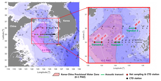
Figure 1.
Map of acoustic transects, net sampling, and CTD stations used for evaluation of the sound scattering layer (SSL) including Euphausia pacifica in the Yellow Sea Bottom Cold Water (YSBCW).

Table 1.
Transect, region, time, start/end position, range, and sea depth information of the acoustic measurements.
2.2. Data Collection
Acoustic measurements were performed using a scientific echosounder system (DT-X Extreme, BioSonics, Inc., Seattle, WA, USA) frequencies of 38 and 200 kHz [30]. The measurement of E. pacifica in the YSBCW was determined using the 38 and 200 kHz. However, the frequencies were mainly used in previous studies of the Yellow Sea [28,29]. Because this study was performed in spring, and given the proliferation of phytoplankton as prey, it was presumed that large numbers of zooplankton would appear in this season; thus, the present study used the frequency of 200 kHz for good resolution in the field acoustic survey.
Before the measurements, the transducers of the echosounder were calibrated in a water tank using 38 mm (38 kHz) and 36 mm (200 kHz) tungsten-carbide calibration spheres and standard procedures [31,32]. After 38 and 200 kHz transducers had been deployed to a small-towed body, it was towed by the research vessel. In order to minimize the effect of ship or surface bubbles by wind, the towed body was located at a depth of roughly 7–9 m from the sea surface to obtain measurements for each transect line (Figure 2, top).
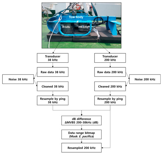
Figure 2.
Flowchart of acoustic data processing using the dB difference method at 38 and 200 kHz.
To identify the regional distribution of E. pacifica, measurements were conducted for three transects at latitudes 35° and 36° in the central, western, and eastern regions (approximately 4 h of measurements for each transect).
Centered on the imaginary midline in the Korea–China provisional water zone (K-C PWZ), the acoustic measurement areas were divided into the central Korea ocean (Transect 1), western China ocean (Transect 2), and eastern Korea exclusive economic zone (EEZ) ocean (Transect 3). The acoustic measurements were performed at sunrise or sunset times for each transect to confirm the DVM pattern of the SSL. Both the 38 and 200 kHz transducers transmitted and received 2 pings/s; the pulse width was 0.5 ms, and the detection range was set at 0–120 m water depth. The threshold level of the received signal was fixed at −100 dB to determine the influence of small organism or zooplankton layers on the volume backscattering strength (Sv). Location information was collected from the differential global positioning system within the echosounder while traveling along the transect lines at a speed of 5–7 knots. The system and environmental parameters of the acoustic measurements are detailed in Table 2.
Table 2.
System parameters of the scientific echosounder used for acoustic surveys in the Yellow Sea Bottom Cold Water.
The ocean environment and net surveys were carried out to understand the ecological characteristics of E. pacifica in the ocean area. Vertical profiles of water temperature were measured at 22 stations (35°, 01–15; 36°, 01–07) using a CTD system (SBE 911plus, Sea-Bird Electronics, Bellevue, WA, USA) from the surface to 5 m above the bottom (Figure 1). The net survey was conducted at five stations: two stations (35°, 10 and 11) in the central region, two stations (35°, 14 and 15) in the western region, and one station (36°, 03) in the eastern region (Figure 1). The net survey was conducted before or after the acoustic transects. The bongo net used for the net survey was a conical net with an attached flowmeter. The bongo net’s diameter, length, and mesh size are 60 cm, 3 m, 200 μm, respectively.
Slope net sampling from the bottom to the surface was performed for approximately 20 min at a net-specific towing speed of 2–3 knots. The samples were fixed immediately using 5% formalin.
After the field surveys, the samples were fixed in formalin and moved to the laboratory. One hundred individuals were randomly selected from each net sampling station, and standard length (L) was measured for 500 specimens obtained through the net surveys at five stations. Because only L was measured and analyzed for these net sampling data, the wet weight (W) was calculated using the W–L relationship of Equation (1) proposed by Kang et al. (2003) [29],
2.3. Acoustic Data Analysis and E. pacifica Identification
The acoustic data collected from the transects were analyzed using acoustic analysis and processing software (Echoview v 9.0; Echoview Ltd., Hobart, Tasmania, Australia). From the acquired Sv of the acoustic measurements, a virtual echogram was generated by removing unnecessary data (e.g., sensor depth, sensor near-field effects, air bubbles in the surface and bottom signals) [33,34]. To understand the DVM of the SSL and identify E. pacifica, the acoustic data were compressed by the horizontal resolution (3.5 s) and the vertical resolution (0.5 m). An analysis and processing flowchart of the acquired acoustic data is shown in Figure 2.
To extract the E. pacifica echoes, this species identification was performed using the difference of the mean volume backscattering strength (∆MVBS) method, which is also known as the dB difference method [35,36,37,38]. The dB difference method depends on the frequency characteristics of the SSL attributable to marine organisms. Generally, zooplankton target strength (TS) is characterized by fluctuations between the low frequency of 38 kHz and the high frequency of 200 kHz [35,39]. Thus, the Sv difference between 38 and 200 kHz is large, providing a good method for species classification. The ∆MVBS window can be used to identify E. pacifica echo signals. By applying the ∆MVBS, other zooplankton (ex. Copepoda) and fish signals were excluded from the net sampling data. The echoes were selected using the data range bitmap algorithm to eliminate noise smaller than the minimum Sv and larger than the maximum Sv of E. pacifica and then masking it by applying the ∆MVBS. E. pacifica were used as the true signals, and all other values were not-selected signals from the data range bitmap (Figure 2). In this study, the range of the ∆MVBS applied (on the basis of biological net sampling data) was 14–19 dB. The range of dB differences used to identify E. pacifica was the recommended range of Sv difference based on the size distribution of E. pacifica by net sampling data.
For the acoustic characteristics of E. pacifica, the TS at 200 kHz was estimated using the distorted wave Born approximation (DWBA) model, a widely used acoustic model for estimating the TS of zooplankton, as shown in Equation (2) [40,41,42],
The ∆MVBS value was obtained by separating the 38 kHz and 200 kHz acoustic signals, using Equation (3),
The swimming speed of DVM of the SSL was estimated by using the echo signal of Sv, to which the ∆MVBS was applied. To calculate the swimming speed, the center of the SSL of each compressed signal was calculated as a function of time D(t). Then, a threshold of −90 dB of Sv was set to accurately extract the center of the SSL. The upward and downward swimming speeds (Vs) were calculated from the rate of change in the SSL as the derivative of D(t) with the time(t) [28],
2.4. Density Estimation of E. pacifica
To estimate the spatially distributed density of E. pacifica, the SSL was separated by excluding fish signals and other zooplankton signals from the acoustic data. The densities by transect of E. pacifica in the SSL were calculated using the ∆MVBS, the Sv, and the nautical area scattering cross-section (NASC) of the 1 nautical mile (n·mile) interval of the elementary distance sampling unit. The density of E. pacifica was calculated via Equation (4) using the L with frequency of L, W–L relationship, and the NASC values obtained from the net sampling data [26,43,44,45],
where is the relative frequency value of E. pacifica concerning the standard length (), and the sum is 1; and are constants calculated from the conversion factor, considering the NASC and W–L relationship. To calculate the mean density () in the survey area, the weighted mean of the data obtained from each transect was used, as in Equation (6):
where N is the number of transect lines, is the mean density of the i-th transect line, and is the distance obtained by converting the i-th transect line into 1 n·mile.
3. Results
3.1. Zooplankton Community Analysis and Size Distribution
According to an analysis of the net sampling data at the five stations, Copepoda was a dominant class with an average of 86%. Euphausiacea and etc. comprised 11% and under 3%, respectively (Figure 3a). It was confirmed that Copepoda consisted of individuals less than 2 mm in L, and Euphausiacea mainly consisted of juvenile and adults of E. pacifica.
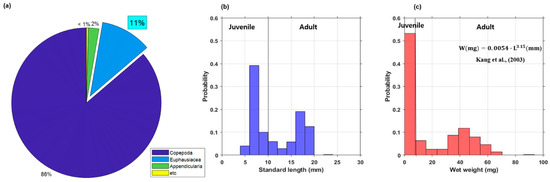
Figure 3.
(a) Zooplankton species composition from net sampling data and the histograms of the (b) standard length (L) frequency distribution and (c) wet weight (W) frequency distribution from all net surveys of E. pacifica in the SSL.
Analysis of the size and weight distribution of E. pacifica was performed using the net survey data; the findings indicated that the juveniles and adults were mixed and distributed concurrently. In the central region, the adult mean L and mean W were 15.1 mm and 33.4 mg, respectively. In contrast, the juvenile mean L and mean W were 6.6 mm and 2.1 mg, respectively. In the western region, the juvenile and adult of mean L and W were 7.2 mm and 2.8 mg, respectively, whereas the juvenile and adult of mean L and W in the eastern region were 17.5 mm and 45.5 mg, respectively. Hence, larger individuals of E. pacifica were caught in the eastern region than at the other net sampling stations. Among five net surveys performed at all net sampling stations, the mean L of E. pacifica was 11.4 mm and the mean W was 19.4 mg.
Large individuals of E. pacifica were found in the eastern region and the Korean oceans; small individuals inhabited the western region. A histogram analysis, performed by dividing the distribution of L of E. pacifica from all net sampling stations by 2 mm, revealed a bimodal distribution ranging from 6 to 8 mm and from 16 to 18 mm (Figure 3b). The highest frequency of W was 0–8 mg (Figure 3c). L and W information obtained via net sampling was used to estimate the density of E. pacifica from the acoustic data.
3.2. DVM of SSL
Figure 4 shows the compressed sample echogram received from the 38 (Figure 4a,c,e) and 200 (Figure 4b,d,f) kHz transducers. The 38 kHz echogram was different from that of the 200 kHz echogram. Despite the shallowness of the ocean, an SSL was formed from E. pacifica and distributed in the YSBCW. Analysis of acoustic data obtained before and after sunrise and sunset revealed that the SSL was distributed at the surface during the nighttime; the DVM findings were characteristic of swimming toward the bottom during the daytime.
In Transect 1 at 200 kHz of the central region, the biological community of the SSL during the nighttime was divided into two layers. At nighttime, an SSL located in the upper layer of the water column was distributed from the surface to a depth of approximately 50 m; an SSL in the lower layer was distributed from a depth of approximately 60 m from the bottom. The upper layer (SSL 1), located at a depth of approximately 25 m, began to swim toward the bottom with a swimming speed of 0.63 m/min from 05:40. The distribution was mixed, with the lower layer (SSL 2) located at a depth of approximately 75 m (Figure 4b).

Figure 4.
Vertical and spatial distributions of the 38 kHz (a,c,e) and 200 kHz (b,d,f) sample echograms for (a,b) Transect 1, (c,d) Transect 2, and (e,f) Transect 3. In the figure, E is east, W is west, black regions are bottom, and depth are divided by 25 m. Daytime and nighttime at the top are divided based on the on-site sunrise and sunset, and the green line is the measured and calculated regions considering the transducer depth, near-field effects, and bottom.

In Transect 2 at 200 kHz in the western region, the SSL was densely distributed near the bottom during the daytime, but it then swam slowly to the surface at the swimming speed of 0.25 m/min. At 20:00, after sunset, the SSL was distributed from the surface layer to a depth of 40 m. As in Transect 1, the SSL in Transect 2 tended to be divided and distributed into two layers (Figure 4d).
In contrast, Transect 3 at 200 kHz in the eastern region exhibited SSL distribution from 40 to 65 m depth during the daytime. From 19:00, before sunset, the SSL moved toward the surface at the swimming speed of 0.40 m/min; it rapidly became densely located at a depth of approximately 20 m after sunset (Figure 4f). The E. pacifica results confirmed DVM during the daytime and nighttime; the downward swimming speed was higher than the upward speed.
3.3. DVM of SSL Vertical Distribution of E. pacifica
The results of the 200 kHz echo signal were comparatively analyzed (Figure 5). In Transect 1, the acoustic signal was highest (−60 dB) at a depth of 60–70 m during the daytime; it was high at a depth of approximately 15–30 m during the nighttime (Figure 5a). In Transect 2, the Sv was high at a depth of approximately 70 m during the daytime, as well as at depths of 30–35 m and 45–60 m during the nighttime (Figure 5b). Conversely, in Transect 3, the Sv was high at a depth of 10–50 m during the nighttime and 45–65 m during the daytime (Figure 5c).
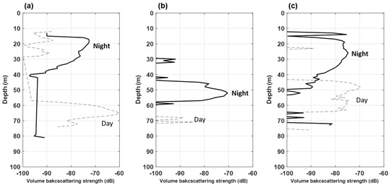
Figure 5.
Variations in mean volume backscattering strength (∆MVBS) of the 200 kHz during daytime and nighttime in the YSBCW at (a) Transect 1, (b) Transect 2, and (c) Transect 3.
The distribution depth of E. pacifica during the nighttime was similar from the acoustic data of Transect 1 and Transect 3. However, the Transect 2 data were densely distributed at a low water depth. The data implied that E. pacifica was densely distributed in the lower layer during the daytime, whereas it was widely distributed from the surface layer to the middle layer during the nighttime. The acoustic data confirmed that the vertical distribution of E. pacifica differed according to the day and night DVM characteristics, as well as the region.
3.4. Density and Spatial Distribution of E. pacifica
Using the dB difference method with the acoustic and net sampling results, DVM patterns in the surface and bottom waters were revealed. The echo signals for Copepoda and fish contained in zooplankton were removed through the ∆MVBS method, and only E. pacifica was extracted. Figure 6 shows the mean density along each transect line. The density was similar when using Sv or NASC. Analysis of the E. pacifica density according to section showed that the E. pacifica density was especially high in the central region, where it was 1.60–55.96 g/m2. In the western and eastern regions, the overall densities were 0.01–9.50 g/m2 and 2.38–25.81 g/m2, respectively. The E. pacifica density in the YSBCW was noticeably higher in the central and eastern regions than in the western region.
The mean E. pacifica densities were 15.78 g/m2, 1.33 g/m2, and 10.26 g/m2, and the coefficients of variation (CV) were 1.14, 1.97, 0.61, respectively, in the central, western, and eastern regions. The overall mean density was 8.33 g/m2. Thus, the SSL had a high-density distribution in the central and eastern regions of the Korean oceans, while it exhibited a low-density distribution in the western region of the YSBCW.

Figure 6.
Calculated densities at each nautical mile, and mean density of E. pacifica in the YSBCW at (a) Transect 1, (b) Transect 2, and (c) Transect 3.
Figure 6.
Calculated densities at each nautical mile, and mean density of E. pacifica in the YSBCW at (a) Transect 1, (b) Transect 2, and (c) Transect 3.

4. Discussion
The YSBCW is formed during the previous winter but remains in the lower layer from spring to late autumn [1,5]. In summer, high temperature and low salinity are distributed at the surface, but low temperature and high salinity are distributed at the bottom in the YSBCW [1]. Therefore, the spatiotemporal distribution of marine organisms in the Yellow Sea is greatly affected by changes in the physical environment, which are related to seasonal changes. In a previous study, E. pacifica exhibited DVM patterns in all water columns from the surface to the bottom in the spring season; it moved to only the lower water column where the thermocline occurred in summer [12]. During the spring season, when the present study was conducted, the water temperature structure of the YSBCW showed a mixed layer from the surface to the bottom; the observed biological characteristics implied SSL movement to the surface and to the bottom through DVM. By applying dB difference, the SSL showing DVM pattern was found to be E. pacifica, and the SSL showing no DVM pattern was removed.
In general, water temperature, salinity, and chlorophyll-a concentration are considered major environmental factors that affect the distribution of E. pacifica [20,21,22]. In the Yellow Sea, E. pacifica is mainly distributed at temperatures lower than 20 °C during the summer [46]; the spatial distribution of E. pacifica is determined primarily by temperature, with a tendency to inhabit cold water (8–16 °C) [23]. Although the net sampling results could not demonstrate a high-resolution SSL pattern (because of the discrete sampling method and net avoidance by E. pacifica), the sampling data provide valuable information for understanding the species composition of the SSL. Therefore, we compared the spatial distribution of temperature with the density of E. pacifica to understand the regional distribution of the YSBCW (Figure 7). The spatial temperature structure obtained from the CTD survey revealed that the difference in temperature between the surface and bottom was within approximately 1 to 4 °C during this period, indicating that all water columns were mixed without significant differences in temperature. The mean temperature was less than approximately 10 °C in the central region (Figure 7b, Transect 1) and less than approximately 8 °C in the eastern region (Figure 7a, Transect 3), except for a portion at the surface; in contrast, a high temperature of approximately 10 °C or higher existed in the western region (Figure 7b, Transect 2). Based on the distribution of water temperature, we concluded that the density of E. pacifica was high in the central and eastern regions because the temperature was lower there than in the western region (less than 10 °C). Therefore, it is assumed that the density of E. pacifica was related to the water temperature.
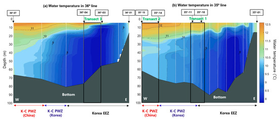
Figure 7.
Spatial distribution of water temperature in the (a) 36° and (b) 35° lines from CTD stations in the YSBCW. In the figure, W is west, E is east, and the depth is divided by 10 m. White dotted lines and grey regions are CTD stations and bottom, respectively.
Thus far, various studies have reported the density or biomass of E. pacifica in the YSBCW, as well as its spatial distribution. In addition to the spatial and temporal distributions of E. pacifica, the estimated density distributions obtained through acoustic and net surveys have been compared with the densities of E. pacifica reported in previous studies. In August 1997 and February 1998, the densities in the northwestern sea of Jeju Island and the central Yellow Sea obtained through net surveys in summer and winter, respectively, were in the range of 39.5–314.7 mg/m3 [20]. In spring 1998, the density of E. pacifica was in the range of 16.5–129.1 mg/m3 [21]. In summer 2002, the density in the East China Sea obtained through acoustic and net surveys was in the range of 20.4–221.4 mg/m3 [29], similar to our results. According to the regular ocean observations of zooplankton biomass conducted from 1978 to 2010 using the net sampling method of the National Institute of Fisheries Science of the Korean government at Korea Oceanographic Data Center stations, the density of E. pacifica in spring was in the range of 10.4–913.9 mg/m3 [47]. Thus, the density shows great variability according to season and year. In an examination of the spatial distribution pattern during the spring of 2006, the mean concentrations of individual eggs, larvae, adults, and juveniles obtained through net surveys in the Yellow Sea were 39.9, 3.58, 0.28, and 0.46 ind./m3 [23], resulting in density range of 0.5–69.2 mg/m3. In that study, egg abundance was positively correlated with chlorophyll-a concentration to a significant degree; the locations of adults were closely correlated with water temperature. In the late spring (May) of 2010, the density of E. pacifica obtained through net surveys in the Yellow Sea was 13.1 ± 14.3 mg/m3 [24]. Kim and Kang (2020) analyzed the density of E. pacifica by net survey in the YSBCW during spring [25]. They reported that the densities in central, western, and eastern regions were in the range of 12.7–495.6 mg/m3, thus revealing some regional differences. According to the acoustic and net surveys in the present study, the density of E. pacifica was in the range of 17.7–210.4 mg/m3. At this time, the density unit of g/m2 was converted to mg/m3 considering the mean depth of 75 m in the YSBCW, and unit of ind./m3 was converted to mg/m3 considering the mean W of E. pacifica.
The density results calculated from the acoustic and net surveys of previous studies provided the same range of values, but some previous results showed a larger variation compared with the density results in the present study. The acoustic survey revealed a high-density distribution of E. pacifica, but quantitative net sampling was difficult because of the strong swimming ability of this species; thus, relative underestimation by net sampling is likely [29]. Table 3 summarizes the density values of E. pacifica according to region, season, and year in the Yellow Sea and the East China Sea, as recorded in previous studies and the present study.
Table 3.
Comparison of E. pacifica density results between previous studies and the present study.
Further studies on more accurate E. pacifica density will be obtained by a multi-frequency technique using 38, 120, 200, and 420 kHz with the dB difference method. If the dB difference method is applied by simultaneously operating various frequencies, it is possible to estimate the density more accurately through the application of the acoustic characteristics for each frequency of E. pacifica. It is planned to estimate the density through acoustic data analysis only during the daytime when the SSL is stably located near the bottom.
On the other hand, the DVM pattern is influenced by environmental and biological factors such as salinity, chlorophyll, suspended solid concentration, nutrient, light intensity, and predator relationship, but we only focused on the water temperature. Therefore, in order to fully understand the DVM mechanism and the characteristics of the regional SSL in the whole YSBCW area, other environmental and biological factors must be investigated in future study.
5. Conclusions
This study proposes the DVM characteristics of the SSL during daytime and nighttime in the YSBCW using hydroacoustic techniques; density characteristics of E. pacifica attributable to regional differences were also identified. In the spring season, E. pacifica showed DVM between the surface and the bottom; upward and downward swimming speeds in the YSBCW were in the range of 0.25–0.63 m/min. The central and eastern regions exhibited a high-density distribution of E. pacifica, while the western region showed a low-density distribution, indicating regional differences. The regional distribution of E. pacifica was related to the water temperature. These results could be used to enhance understanding of the marine ecosystem structure of the YSBCW.
Author Contributions
Conceptualization, H.K. and D.K.; methodology, H.K. and D.K.; formal analysis, H.K., G.K. and M.K.; investigation, H.K., G.K. and D.K.; writing—original draft preparation, H.K. and D.K. All authors have read and agreed to the published version of the manuscript.
Funding
This research was conducted with the support of the research project of “Research based on Understanding and Response to Changes in Marine Ecosystems in the Adjacent Sea of Korea (PE99913)” funded by the Korea Institute of Ocean Science and Technology (KIOST) and “Development of Marine Science Exploration Technology in Coastal areas (PM62603)” funded by the Ministry of Oceans and Fisheries (MOF), Korea.
Institutional Review Board Statement
Not applicable.
Informed Consent Statement
Not applicable.
Data Availability Statement
The data presented in this study are available on request from the corresponding author. The data are not publicly available since the data also forms part of an on- going study.
Acknowledgments
We are grateful to Seok Lee, other scientists, and crew members of “R/V Onnuri” in the Korea Institute of Ocean Science and Technology (KIOST).
Conflicts of Interest
The authors declare no conflict of interest.
References
- Lie, H.J. A note on water masses and general circulation in the Yellow Sea. J. Oceanol. Soc. Korea 1984, 19, 187–194. (In Korean) [Google Scholar]
- Teague, W.J.; Jacobs, G.A. Current observations on the development of the Yellow Sea warm current. J. Geophys. Res. 2000, 105, 3401–3411. [Google Scholar] [CrossRef]
- Park, Y.H. Water characteristics and movements of the Yellow Sea Warm Current in summer. Prog. Oceanogr. 1986, 17, 243–254. [Google Scholar] [CrossRef]
- Lie, H.J.; Cho, C.H.; Lee, S. Tongue-shaped frontal structure and warm water intrusion in the southern Yellow Sea in winter. J. Geophys. Res. Ocean. 2009, 114, C01003. [Google Scholar] [CrossRef]
- Hur, H.B.; Jacobs, G.A.; Teaque, W.J. Monthly variations of water masses in the Yellow and East China seas. J. Oceanogr. 1999, 55, 171–184. [Google Scholar] [CrossRef]
- Jang, S.T.; Lee, J.H.; Kim, C.H.; Jang, C.J.; Jang, Y.S. Movement of cold water mass in the Northern East China Sea in summer. Sea J. Korean Soc. Oceanogr. 2011, 16, 1–13. (In Korean) [Google Scholar]
- Food and Agriculture Organization (FAO). Fishery Production Statistics. 2020. Available online: http://www.fao.org/home/en/ (accessed on 1 March 2021).
- Ministry of Oceans and Fisheries (MOF). Fisheries Production Statistics, Ministry of Oceans and Fisheries. 2020. Available online: https://www.mof.go.kr/en/index.do/ (accessed on 17 October 2020).
- Jang, M.; Jo, H.; Kweon, D.; Cha, B.; Hwang, J.; Han, K.; Im, Y. Geographical distribution and catch fluctuations of Mottled skate, Beringraja pulchra in the eastern Yellow sea. Korean J. Ichthyol. 2014, 26, 295–302. (In Korean) [Google Scholar]
- Everson, I. The Southern Ocean. In Krill Biology, Ecology and Fisheries; Everson, I., Ed.; Blackwell Science Oxford: London, UK, 2008; pp. 63–79. ISBN 9780470999486. [Google Scholar]
- Kim, Y.S.; Choi, J.H.; Kim, J.N.; Oh, T.Y.; Choi, K.H.; Lee, D.W.; Cha, H.K. Seasonal variation of fish assemblage in Sacheon marine ranching, the southern coast of Korea. J. Korean Soc. Fish Technol. 2010, 46, 335–345. [Google Scholar] [CrossRef]
- Lee, H.; Cho, S.; Kim, W.; Kang, D. The diel vertical migration of the sound-scattering layer in the Yellow Sea Bottom Cold Water of the southeastern Yellow sea: Focus on its relationship with a temperature structure. Acta Oceanol. Sin. 2013, 32, 44–49. [Google Scholar] [CrossRef]
- Zaret, T.M.; Suffern, J.S. Vertical migration in zooplankton as a predator avoidance mechanism. Limnol. Oceanogr. 1976, 21, 804–813. [Google Scholar] [CrossRef]
- Forward, R.B. Diel vertical migration: Zooplankton photobiology and behaviour. Oceanogr. Mar. Biol. Annu. Rev. 1988, 26, 361–393. [Google Scholar]
- Berge, J.; Cottier, F.; Varpe, Ø.; Renaud, P.E.; Falk-Petersen, S.; Kwasniewski, S.; Griffiths, C.; Søreide, J.E.; Johnsen, G.; Aubert, A.; et al. Arctic complexity: A case study on diel vertical migration of zooplankton. J. Plankton Res. 2014, 36, 1279–1297. [Google Scholar] [CrossRef] [PubMed]
- Lampert, W. The adaptive significance of diel vertical migration of zooplankton. Funct. Ecol. 1989, 3, 21–27. [Google Scholar] [CrossRef]
- Murphy, H.M.; Jenkins, G.P.; Hamer, P.A.; Swearer, S.E. Diel vertical migration related to foraging success in snapper Chrysophrys auratus larvae. Mar. Ecol. Prog. Ser. 2011, 433, 185–194. [Google Scholar] [CrossRef]
- Zhou, M.; Dorland, R.D. Aggregation and vertical migration behavior of Euphausia superba. Deep Sea Res. Part II Top. Stud. Oceanogr. 2004, 51, 2119–2137. [Google Scholar] [CrossRef]
- Gaten, E.; Tarling, G.; Dowse, H.; Kyriacou, C.; Rosato, E. Is vertical migration in Antarctic krill (Euphausia superba) influenced by an underlying circadian rhythm? J. Genet. 2008, 87, 473–483. [Google Scholar] [CrossRef] [PubMed][Green Version]
- Yoon, W.D.; Cho, S.H.; Lim, D.H.; Choi, Y.K.; Lee, Y. Spatial distribution of Euphausia pacifica (Euphausiacea: Crustacea) in the Yellow Sea. J. Plankton Res. 2000, 22, 939–949. [Google Scholar] [CrossRef][Green Version]
- Yoon, W.D.; Yang, J.Y.; Lim, D.; Cho, S.H.; Park, G.S. Species composition and spatial distribution of euphausiids of the Yellow Sea and relationships with environmental factors. Ocean Sci. J. 2006, 41, 11–29. [Google Scholar] [CrossRef]
- Liu, H.L.; Sun, S. Diel vertical distribution and migration of a euphausiid Euphausia pacifica in the Southern Yellow Sea. Deep Sea Res. Part II Top. Stud. Oceanogr. 2010, 57, 594–605. [Google Scholar] [CrossRef]
- Sun, S.; Tao, Z.; Li, C. Spatial distribution and population structure of Euphausia pacifica in the Yellow Sea (2006–2007). J. Plankton Res. 2011, 33, 873–889. [Google Scholar] [CrossRef]
- Zuo, T.; Liu, H. Seasonal size composition and abundance distribution of Euphausia pacifica in relation to environmental factors in the southern Yellow Sea. Acta Oceanol. Sin. 2019, 38, 70–77. [Google Scholar] [CrossRef]
- Kim, G.; Kang, H.K. Mesozooplankton community structure in the Yellow Sea in Spring. Ocean Polar Res. 2020, 42, 271–281. (In Korean) [Google Scholar] [CrossRef]
- Simmonds, E.J.; MacLennan, D.N. Fisheries Acoustics: Theory and Practice, 2nd ed.; Blackwell Science: Oxford, UK, 2005; pp. 1–437. ISBN 9780632059942. [Google Scholar]
- Lü, L.-G.; Liu, J.; Yu, F.; Wu, W.; Yang, X. Vertical migration of sound scatterers in the southern Yellow Sea in summer. Ocean Sci. J. 2007, 42, 1–8. [Google Scholar] [CrossRef]
- Lee, M.A.; Chao, M.H.; Weng, J.S.; Lan, Y.C.; Lu, H.J. Diel distribution and movement of sound scattering layer in Kuroshio waters, northeastern Taiwan. J. Mar. Sci. Technol. 2011, 19, 253–258. [Google Scholar] [CrossRef]
- Kang, D.; Hwang, D.J.; Soh, H.Y.; Yoon, Y.H.; Suh, H.L.; Kim, Y.J.; Shin, H.C.; Iida, K. Density estimation of Euphausiid (Euphausia pacifica) in the sound scattering layer of the East China sea. J. Korean Fish. Soc. 2003, 36, 749–756. (In Korean) [Google Scholar]
- BioSonics. Visual Acquisition DT-X User Guide, Version 3.37; BioSonics: Seattle, WA, USA, 2019; pp. 1–64. [Google Scholar]
- BioSonics. Calibration Manual (Wireless Scienfitic Echo Sounder DT-X Series), Version 2; BioSonics: Seattle, WA, USA, 2004; pp. 1–23. [Google Scholar]
- Svein, V.; Kenneth, F.; Mark, T.; David, F. A technique for calibration of monostatic echosounder systems. IEEE J. Ocean. Eng. 1996, 21, 298–305. [Google Scholar]
- De Robertis, A.; Higginbottom, I. A post-processing technique for estimation of signal-to-noise ratio and removal of echosounder background noise. ICES J. Mar. Sci. 2007, 64, 1282–1291. [Google Scholar] [CrossRef]
- Ryan, T.E.; Downie, R.A.; Kloser, R.J.; Keith, G. Reducing bias due to noise and attenuation in open-ocean echo integration. ICES J. Mar. Sci. 2015, 72, 2482–2493. [Google Scholar] [CrossRef]
- Miyashita, K.; Aoki, I.; Seno, K.; Taki, K.; Ogishima, T. Acoustic identification of isada krill, Euphausia pacifica Hansen, off the Sanriku coast, north-eastern Japan. Fish. Oceanogr. 1997, 6, 266–271. [Google Scholar] [CrossRef]
- Kang, M.H.; Furusawa, M.; Miyashita, K. Effective and accurate use of difference in mean volume backscattering strength to identify fish and plankton. ICES J. Mar. Sci. 2002, 59, 794–804. [Google Scholar] [CrossRef]
- Watkins, J.L.; Brierley, A.S. Verification of the acoustic techniques used to identify Antarctic krill. ICES J. Mar. Sci. 2002, 59, 1326–1336. [Google Scholar] [CrossRef]
- Kang, M.H.; Fajaryanti, R.; Son, W.; Kim, J.-H.; La, H.S. Acoustic detection of krill scattering layer in the Terra Nova Bay Polynya, Antarctica. Front. Mar. Sci. 2020, 7, 1013. [Google Scholar] [CrossRef]
- Korneliussen, R.J.; Ona, E. Synthetic echograms generated from the relative frequency response. ICES J. Mar. Sci. 2003, 60, 636–640. [Google Scholar] [CrossRef]
- McGehee, D.E.; O’Driscoll, R.L.; Traykovski, L.M. Effects of orientation on acoustic scattering from Antarctic krill at 120 kHz. Deep Sea Res. Part II Top. Stud. Oceanogr. 1998, 45, 1273–1294. [Google Scholar] [CrossRef]
- Demer, D.A.; Conti, S.G. Reconciling theoretical versus empirical target strengths of krill: Effects of phase variability on the distorted-wave Born approximation. ICES J. Mar. Sci. 2003, 60, 429–434. [Google Scholar] [CrossRef]
- Bairstow, F.; Gastauer, S.; Finley, L.; Edwards, T.; Brown, C.T.; Kawauchi, S.; Cox, M.J. Improving the Accuracy of Krill Target Strength Using a Shape Catalog. Front. Mar. Sci. 2021, 8, 290. [Google Scholar] [CrossRef]
- Hewitt, R.P.; Demer, D.A. Dispersion and abundance of Antarctic krill in the vicinity of Elephant Island in the 1992 austral summer. Mar. Ecol. Prog. Ser. 1993, 99, 29–39. [Google Scholar] [CrossRef]
- Reiss, C.S.; Cossio, A.M.; Loeb, V.; Demer, D.A. Variations in the biomass of Antarctic krill (Euphausia superba) around the South Shetland Islands, 1996–2006. ICES J. Mar. Sci. 2008, 65, 497–508. [Google Scholar] [CrossRef]
- Choi, S.G.; Chae, J.; Chung, S.; Oh, W.; Yoon, E.; Sung, G.; Lee, K. Density estimation of Antarctic krill in the south Shetland Island (subarea 48.1) using dB-difference method. Sustainability 2020, 12, 5701–5715. [Google Scholar] [CrossRef]
- Iguchi, N.; Ikeda, T. Experimental study on brood size, egg hatchability, and early development of a euphausiid Euphausia pacifica from Toyama Bay, Southern Japan Sea. Bull. Jpn. Sea Natl. Fish. Res. Inst. 1994, 44, 49–57. [Google Scholar]
- Choi, J.W.; Park, W.G. Variations of Marine Environments and Zooplankton Biomass in the Yellow Sea during the Past Four Decades. J. Mar. Sci. Eng. 2013, 25, 1046–1054. (In Korean) [Google Scholar]


Publisher’s Note: MDPI stays neutral with regard to jurisdictional claims in published maps and institutional affiliations. |
© 2022 by the authors. Licensee MDPI, Basel, Switzerland. This article is an open access article distributed under the terms and conditions of the Creative Commons Attribution (CC BY) license (https://creativecommons.org/licenses/by/4.0/).