Hydrodynamic Modelling of Wave Overtopping over a Block-Covered Flood Defence

Abstract

Wave overtopping can cause erosion on the landward slope due to high flow velocities and turbulence that cause high stresses on the cover. Innovative block revetments such as Grassblocks protect the subsoil of the dike against erosion. The blocks are permeable, which reduces the flow velocity and the pressures along the landward slope. The performance of these blocks is assessed in physical tests, which provides insights into the stability of the blocks. However, such experiments are expensive and accurate measurements are difficult due to highly turbulent conditions. Therefore, the goal of this study is to determine the hydrodynamic conditions at the dike cover caused by the wave run-up on the seaward slope and by the overtopping flow over the crest and landward slope. The geometry and wave conditions from the physical test at the Deltares Delta flume are implemented in an OpenFOAM^® numerical model. Using the porousWaveFoam solver, a porous layer on the crest and landward slope is implemented, where the flow resistance of this porous layer largely depends on the resistance coefficients $\alpha$ [-] and $\beta$ [-]. The numerical model is calibrated based on resistance coefficients as introduced earlier in the literature, which showed that the resistance coefficients of $\alpha =500$ and $\beta =2.0$ performed best for the peak flow velocities and the peak pressures. The numerical model is evaluated by using these resistance coefficients in other time series of the physical tests. The evaluated model is then used to determine the hydrodynamic conditions on the landward slope, which showed that the pressure was the most influential hydrodynamic condition at the time of failure. Finally, the model showed that a porosity of $n=0.6$ and the porous layer thickness $\eta =36\mathrm{mm}$ reduced the peak pressure the most.

1. Introduction

Wave overtopping is one of the main failure mechanisms of dikes. The wave overtopping process consists of three different phases: wave impact, wave run-up, and wave overtopping. The waves can overtop over the dikes during storm events. When the water reaches the seaward slope, crest, or landward slope of the dike, it can cause erosion due to high flow velocities and turbulence [1,2,3,4]. Dike cover erosion due to wave loads by overtopping waves could eventually lead to dike breaching, which can result in severe losses of properties and lives. Experiments [5,6,7,8,9,10] and numerical models [11,12] have shown that erosion on dikes is mainly caused by wave loads, such as pressure, normal stress, shear stress and flow velocities. Therefore, accurate estimations of these wave loads are important for dike designs and safety assessments.

Innovative covers strengthen the earthen dike cover against wave run-up and overtopping flow. When the grass cover erodes during extreme storm events, the blocks will still protect the underlying subsoil of the dike against erosion by overtopping waves (Figure 1). Blocks such as Grassblocks (Figure 2) have an open volume between the blocks to absorb the up- and down-rushing water and dissipate the wave energy. This open volume per square meter defines the porosity of the system. Physical overtopping tests were performed to assess the performance of these blocks [13]. These large-scale physical tests provide insights into the stability of the blocks, but such tests are expensive. Furthermore, it is difficult to measure the flow conditions, such as flow velocity and pressure due to the highly turbulent conditions and the limited number of measuring locations. Additionally, it is time consuming to change the dike configurations in the physical tests.

Numerical models can provide the flow characteristics on any location on the dike cover and, therefore, can provide insight into the flow conditions on the dike and the limits of the dike cover. Previous research, e.g., Jacobsen et al. [15], Van Bergeijk et al. [16], and Chen et al. [17], has shown the capability of hydrodynamic numerical modelling in simulating the wave overtopping flow. However, these models were applied to simulate the flow on the waterside of the flood defence [15,17,18] or on the landward side [11,16]. The models for the landward slope use empirical volume distributions at the dike crest as the input for modelling the wave load along the landward slope, which can lead to inaccurate estimations of the wave load. Furthermore, the connection to the design conditions such as the water level and wave height is missing in these landward slope models. A hydrodynamic numerical model that has been validated for accurately simulating the hydrodynamic conditions due to wave overtopping over the waterside slope, crest, and landward slope of dikes, including permeable block revetments, does not exist yet. Therefore, the main goal of this paper is to make a reliable model for predicting the wave overtopping load along the dike cross-section and to use this model to quantify the physical stresses during the wave overtopping process. Using this new numerical model, we will access the strongest configuration of porous layer thickness and porosity of the block revetment in order to protect the dike against wave overtopping erosion.

For that purpose, a 2DV numerical model was set up using OpenFOAM®, in which a porous layer was implemented to represent the porosity of the Grassblock revetment. The OpenFOAM® model was calibrated and evaluated by comparing the numerically modelled flow velocities and pressures with the experimental data of the large-scale physical tests of Van Steeg [13]. The evaluated numerical model was then applied to determine the optimal configuration of the block revetment for reducing the overtopping forces.

The paper is structured as follows: Section 2 describes the physical model set-up, whereas Section 3 shows the numerical model set-up, calibration, and evaluation. In Section 4, the results are presented followed by the discussion and the conclusions in Section 5 and Section 6, respectively.

2. Physical Model Tests

Two flume tests were performed in the Deltares Delta flume by Van Steeg [13] to determine the strength of the Grassblock against the wave forces. The waves were generated using a wave paddle that can generate regular and irregular waves with a significant wave height $H_s$ up to $2.0\mathrm{m}$ and is equipped with an active wave absorption system that prevents wave reflection [19]. Figure 3 shows the test set-up with the location of the wave generator paddle, the dike, the wave height meters, and the flow velocity and pressure sensors along the dike crest and landward slope. The toe of the dike structure was located at a cross-flume distance of $X=164.19\mathrm{m}$. The lower waterside slope of the dike consists of concrete, followed by a section of Grassblocks ($X=190.29\mathrm{m}$, $Z=8.95\mathrm{m}$) on the waterside slope covering the crest until the landward slope ($X=201.79\mathrm{m}$, $Z=6.20\mathrm{m}$). The Grassblocks that were used in this study are permeable and were installed on a layer of geotextile with a clay layer of $0.4$ m underneath [13]. The free surface elevation of the waves was measured by three wave height meters (also referred to as wave gauges) located at $108.5$ m, $114.5$ m, and $117.5$ m, respectively, from the wave paddle.

The flow velocity was measured with a frequency of 100 Hz by two paddle wheels (PW) which were installed on the landward slope of the dike (Figure 3b). The centres of the paddle wheels were located at 27 mm above the top of the Grassblocks. The pressure was measured on five locations on the dike by pressure sensors (PS) with a frequency of $100$ Hz. The pressures at PS2–PS5 were measured at 8 mm above the top of the Grassblocks and at 30 cm from the wall of the flume.

The test program consisted of two different tests in which the wave load was increased by increasing the wave height and reducing the wave steepness, see

Table 1. The wave characteristics during the two tests with the water depth h, significant wave height $H_{m0}$, maximum wave height $H_{max}$, peak wave period $T_p$, spectral wave period $T_{m-1,0}$, wave steepness $s_{m-1,0}$, and number of waves N.

Test	h	${\mathit{H}}_{\mathit{m}0}$	${\mathit{H}}_{\mathit{max}}$	${\mathit{T}}_{\mathit{p}}$	${\mathit{T}}_{\mathit{m}-1,0}$	${\mathit{s}}_{\mathit{m}-1,0}$	q	N
	[m]	[m]	[m]	[s]	[s]	[−]	[l/s/m]	[−]
Test A	6.9	1.48	2.66	4.89	4.54	0.046	9.3	1032
Test B	6.9	1.63	2.36	7.23	6.53	0.024	34.2	54

. The irregular waves were generated based on the JONSWAP spectrum. The forces on the blocks were only caused by water flowing over the blocks, because the overtopping water did not separate at the landward crest line and therefore the blocks did not experience any impact forces (Figure 4a). After Test A, no damage was observed on the Grassblocks. After one critical overtopping wave at 300 s in Test B the Grassblocks collapsed after which this test was aborted (Figure 4b). The collapse started at the toe of the landward slope, directly followed by the collapse of the block formation from the landward toe towards the crest.

3. Method

The measurements of the physical wave overtopping tests by Van Steeg [13] are used to set-up, calibrate, and evaluate the numerical model for a range of wave load conditions. After the evaluation, the hydraulic loads on the blocks were determined using the numerical model to determine the block revetment specifications leading to the smallest hydraulic forces. This section gives a description of the model set-up (Section 3.1), model calibration (Section 3.2), model evaluation (Section 3.3), and hydraulic loads on the blocks (Section 3.4).

3.1. Numerical Model Set-Up

OpenFOAM® 1712 was used in this study to set up the numerical model. OceanWave3D coupled with the waves2Foam toolbox developed by Jacobsen et al. [15] was used to generate the same waves in the numerical model as those in the physical model tests. Detailed information about the coupling approach can be found in Paulsen et al. [20]. The movement of the wave paddle at the Deltares Delta flume is controlled by a steering file that describes the movement of the wave paddle to generate the wave time series. The steering files were used to translate the movement of the wave paddle into the OpenFOAM® model using OceanWave3D [21]. Since the Grassblocks that were used in this study are permeable, the Volume-averaged Reynolds-averaged Navier–Stokes (VRANS) equations were solved using the porousWaveFoam solver [18], which is included in the waves2Foam toolbox using the resistance coefficients $\alpha$ and $\beta$ (see Appendix A).

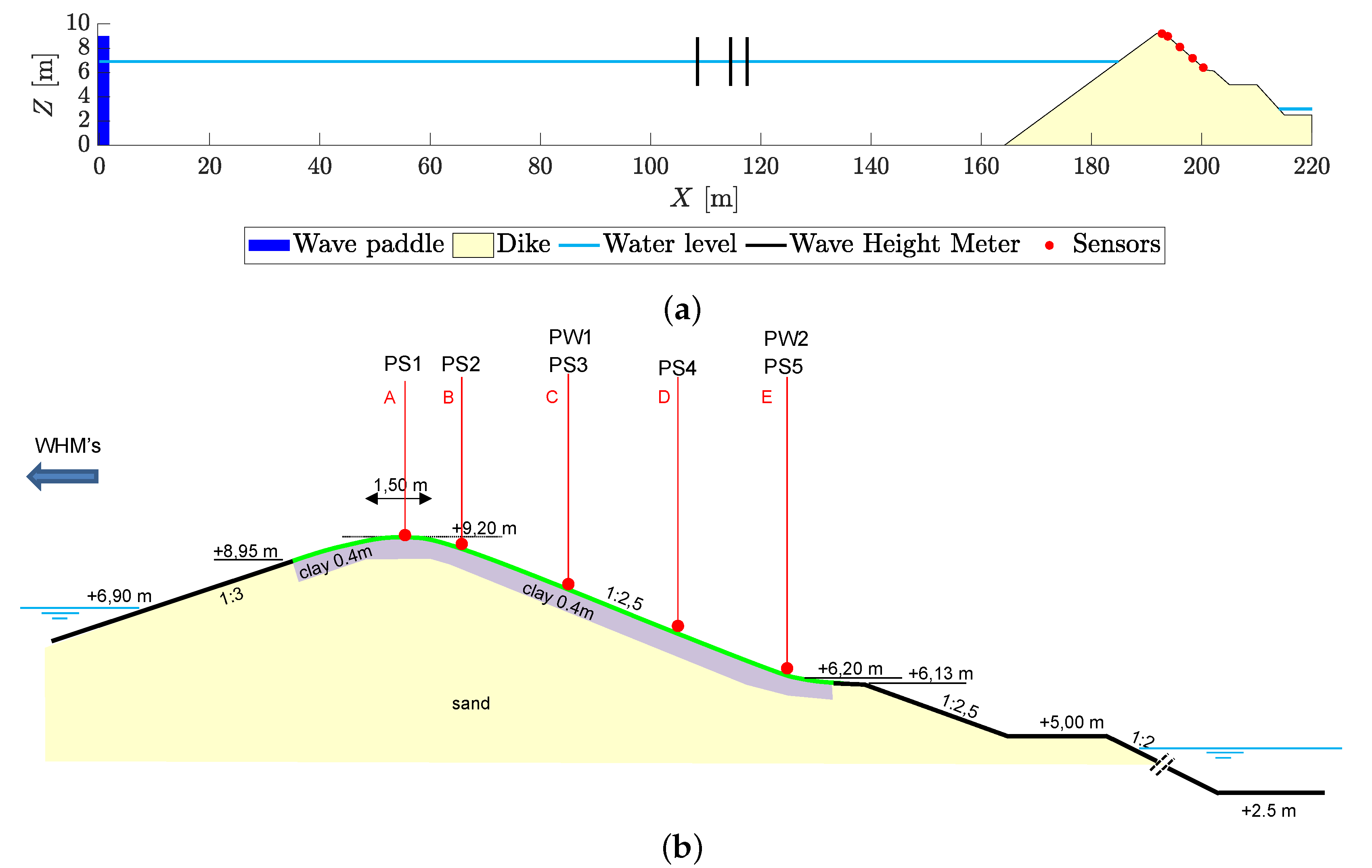
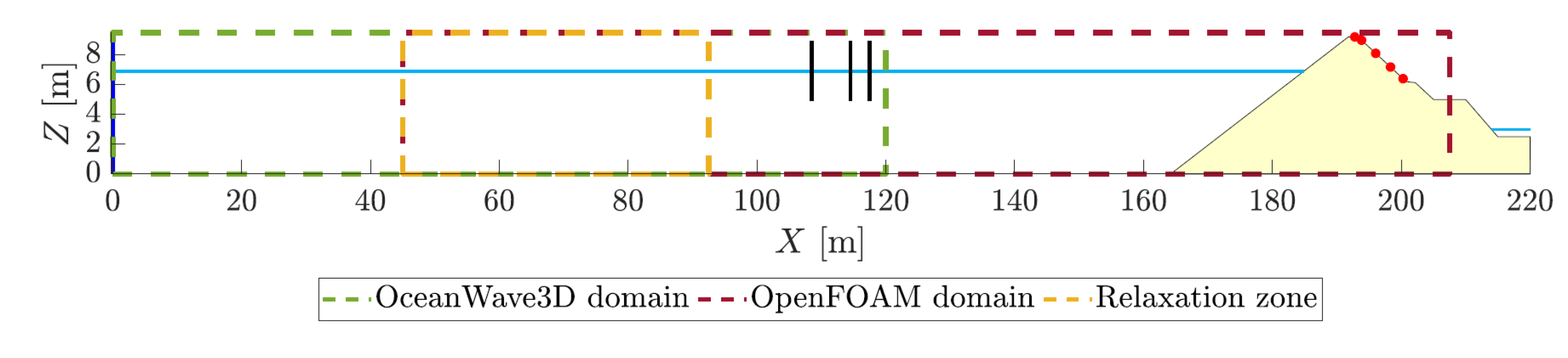
The dike geometry was implemented into the OpenFOAM® model using blockMesh (Figure 5). The flume in the numerical model starts at $42.5$ m away from the wave generator up to 206 m with a height of $12.1$ m. The relaxation zone avoids internally reflecting waves at the wave generating boundary of the numerical model. The length of the relaxation zone was set as close to one wavelength [22].

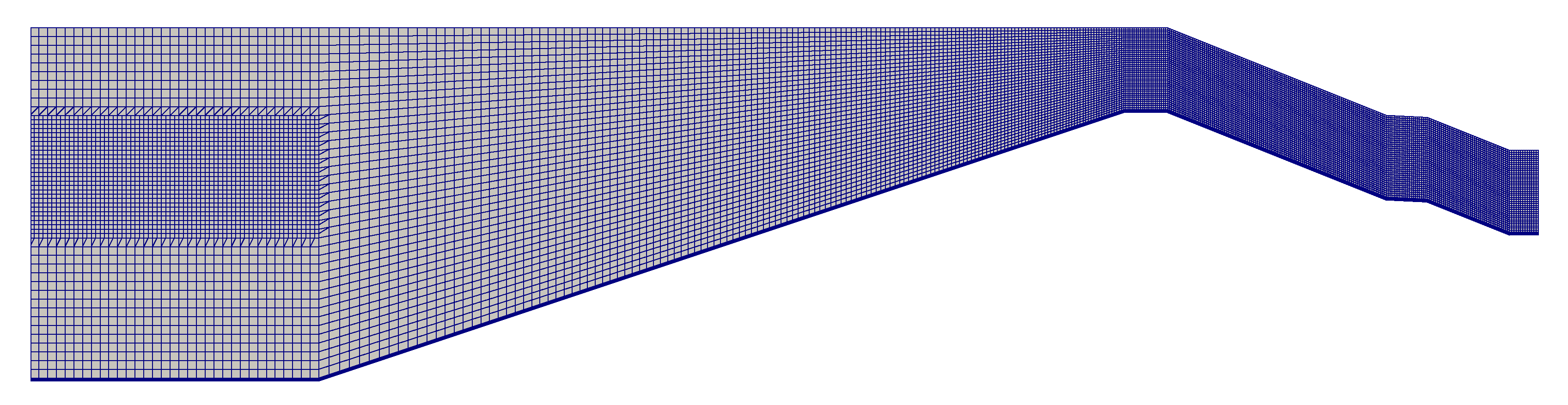
According to Jacobsen et al. [15] and Pedersen et al. [23], maintaining an aspect ratio of $\Delta x/\Delta z=1$ throughout the computational domain improves the accuracy and numerical stability of the model. The mesh size is 30 × 30 cm, leading to 40 cells in the vertical direction. The mesh size on the crest and landward slope is 7 × 7 cm. Similar to the research by Chen et al. [17], a wall function was used in the boundary layer near the bottom surface of the flume. The mesh was refined near the bottom along the entire domain using 10 cells with a height of 1 cm to simulate the vertical velocity profile accurately.

Windt et al. [24] have shown that 10 layers of cells per wave height are needed to resolve the wave height accurately. The significant wave height varies from $1.48$ m up to $1.69$ m. With a minimum of 10 vertical layers per wave height, this leads to a mesh size of 15 × 15 cm. Therefore, the grid was locally refined near the water surface from $Z=4.9$–$8.9\mathrm{m}$ in vertical direction and from the start of the flume until the start of the slope ($X=42.5$–$164.19\mathrm{m}$) in horizontal direction (Figure 6). The maximum Courant number was set to 0.25 as Gruwez et al. [25] showed that $C=0.25$ led to a good balance between accuracy and computational costs.

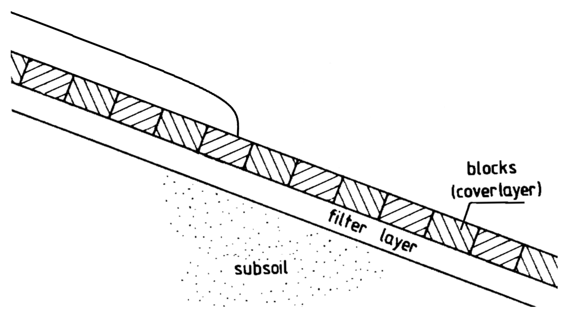
The porous zones are defined by resistance properties and were implemented into OpenFOAM® using porosityZones. The porous zone starts near the top of the waterside slope ($X=191.04$ m, $Z=8.95$ m) and ends at the toe of the landward slope ($X=201.79$ m, $Z=6.2$ m). The porous zone has a depth of 36 mm over the whole layer, which is the same height as the open top part of the Grassblocks so that only the porous part of the blocks is implemented as porous layer in the numerical model. Furthermore, the porosity of $n=0.4$ is used in the numerical model based on the ratio of void volume out of the total volume on the upper 36 mm of the Grassblock.

Van Gent [26] proposed the resistance coefficients $\alpha =1000$ and $\beta =1.1$ based on measurements of the permeability during experiments with porous flows through rubble-mound material. Losada et al. [27] showed that the resistance coefficients depend on parameters such as the Reynolds number, the shape of the stones, the grade of the porous material, and the permeability and the flow characteristics. However, the precise descriptions of the $\alpha$ and $\beta$ coefficients are still not fully understood for oscillatory flows in wave propagation and breaking over slopes [27]. For these conditions, the values as proposed in literature may not be valid since the experimental conditions for obtaining those formulae were not considering these effects. Based on a comparison of experimental data and numerical modelling results of wave overtopping processes (COBRAS-UC), Losada et al. [27] proposed $\alpha =200$ and $\beta =0.8$ as the best-fit parameters in his research. Furthermore, Jensen et al. [18] compared experimental data with numerical outcomes. Based on research by Burcharth and Andersen [28], Jensen et al. [18] proposed that the Reynolds number in porous media $R{e}_p$ can be determined using Equation (1).

$$R{e}_p=\frac{\langle \overline{u}\rangle d_{50}}{n\nu }$$

(1)

Based on this Reynolds number, a distinction was made by Jensen et al. [18] for different flow regimes. The first is a non-linear flow regime, also described as the Forchheimer flow regime ($10<R{e}_p<150$). The second is an unsteady laminar flow regime, also called the transitional flow regime ($150<R{e}_p<300$). The last one is the fully turbulent flow regime, with $R{e}_p>300$. According to Jensen et al. [18], the resistance coefficients $\alpha =500$ and $\beta =2.0$ performed best considering all flow regimes.

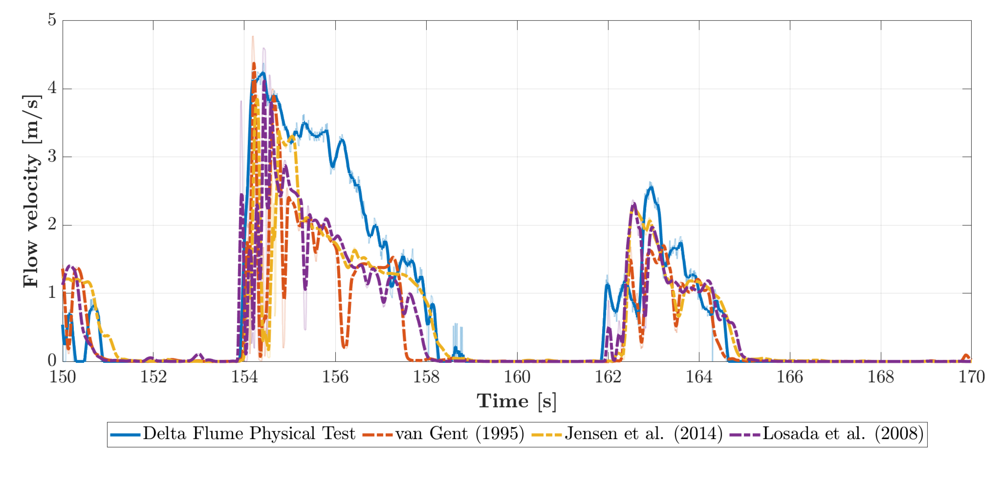
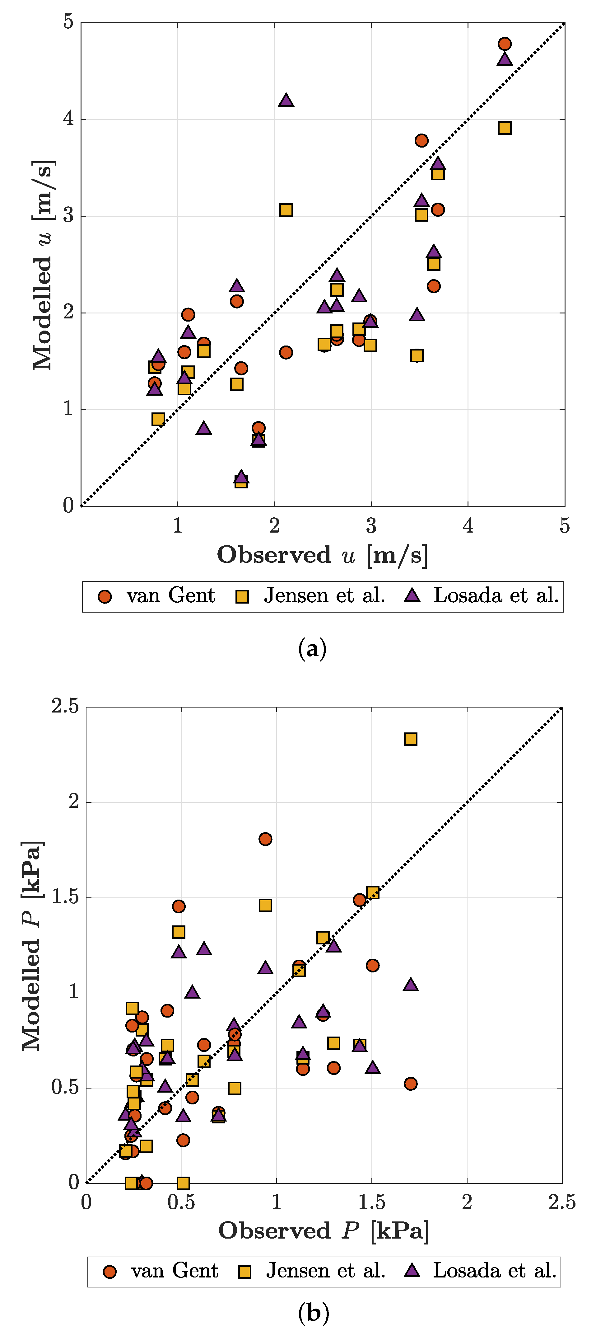
Three different sets of resistance coefficients were selected based on Van Gent [26], Losada et al. [27], Jensen et al. [18] to calibrate the numerical model, as displayed in

Table 2. Resistance coefficients $\alpha$ and $\beta$ used in different studies.

Study	$\mathit{\alpha }$	$\mathit{\beta }$
Van Gent [26]	1000	1.1
Jensen et al. [18]	500	2.0
Losada et al. [27]	200	0.8

.

Since wave breaking was observed in the physical experiments, the turbulence should be accounted for in the numerical model. The stabilised $k-\omega$ turbulence model developed by Larsen and Fuhrman [29] was used in this study, where k is the turbulent kinetic energy [m²/s²] and $\omega$ the specific rate of dissipation of turbulent kinetic energy. The $k-\omega$ turbulence model has a stress limiter ${\lambda }_1$ and an effective potential flow threshold ${\lambda }_2$. Larsen and Fuhrman [29] suggested a value of ${\lambda }_2=0.05$ and for ${\lambda }_1$ either 0.2 and 0.875 is mentioned. Chen et al. [17] showed that ${\lambda }_1=0.2$ performed better in a $k-\omega$ model for wave overtopping. The stabilised $k-\omega$ model with ${\lambda }_1=0.2$ and ${\lambda }_2=0.05$ was used in this study.

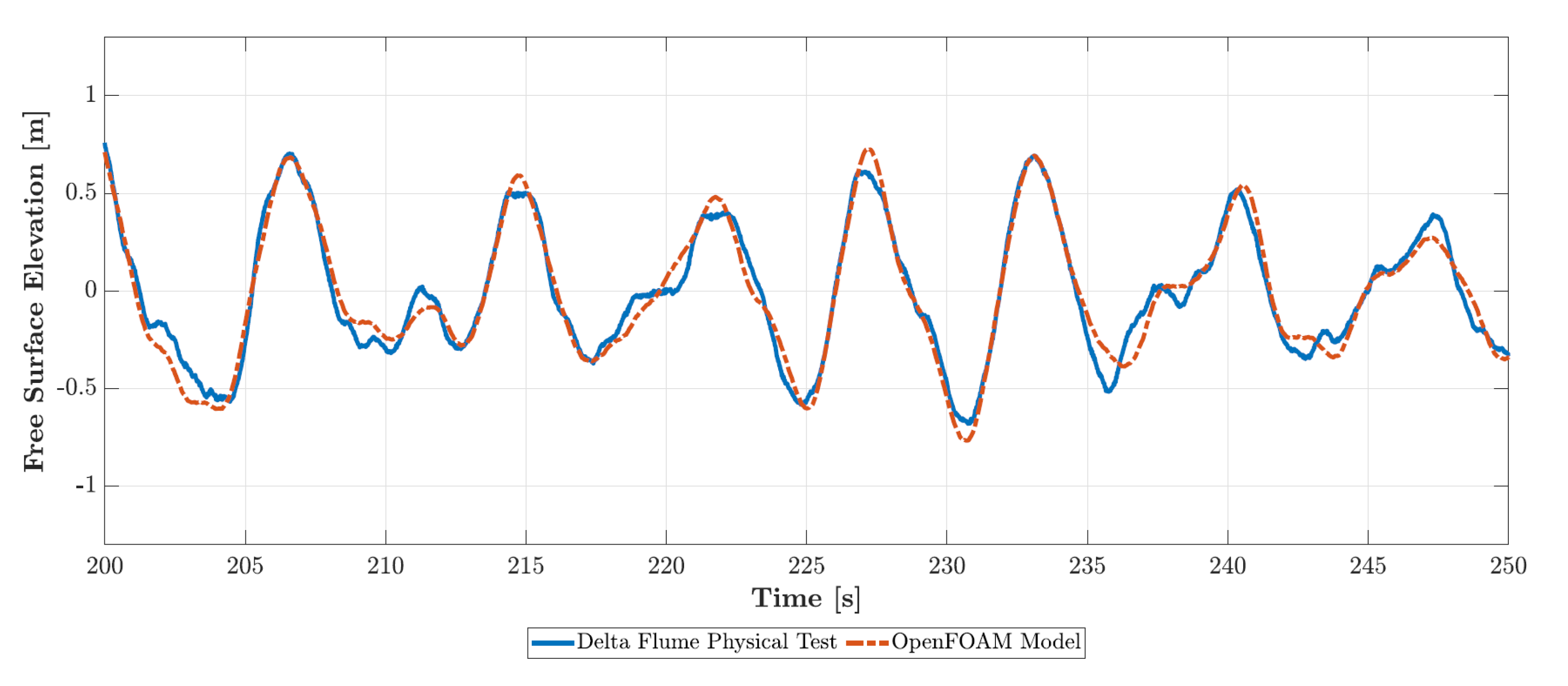
The generated waves were calibrated following the approach of Chen et al. [17] to ensure that the modelled waves accurately represent the waves from the physical experiment. Wave height meters were defined in the numerical model at the same location as used in the physical experiment. Using the wave separation method of Mansard and Funke [30], the spectral density of the free surface elevation was determined. Based on the $m_0$ and $m_{-1}$ moment of the spectral density, the significant wave height $H_{m0}=4\sqrt{m_0}$ and spectral wave period $T_{m-1,0}=m_{-1}/m_0$ were obtained. The waves were then calibrated by comparing $H_{m0}$ and $T_{m-1,0}$ of the numerical model simulated waves and the physical test waves.

3.2. Calibration of the Resistance Coefficients

The pressures and flow velocities were calculated in OpenFOAM® using probes at the same locations as the pressure sensor and paddle wheels in the physical test. The first half of Test B ($t=0$–$170$ s) was used for calibration. The peak flow velocity and peak pressure of each overtopping wave were assessed, because the peak values of the flow velocity and pressure have the most influence on the stability of the dike cover. An overtopping wave was defined as the exceedance of a minimum pressure of 0.2 kPa and a minimum flow velocity of 0.5 m/s. The modelled peak pressures and velocities of each run with resistance coefficients from Van Gent [26], Jensen et al. [18], and Losada et al. [27] were compared with the peak pressures and velocities as measured in the physical tests. The goodness of the obtained fits for each set of resistance coefficients are scored using the Nash–Sutcliffe Efficiency (NSE) and the root-mean-square error (RMSE), which are often used in previous studies (e.g., Chen et al. [31], Van Bergeijk et al. [4], and Van Gent [32]). A perfect fit between the model results and the formulation results in a NSE of 1 and a NSE of 0 indicates that the formulation is as accurate as the mean of the model results [33]. The RMSE shows the average deviation of the modelled values compared to the observed values. The resistance coefficient set with the highest NSE and smallest RMSE is selected for the further simulations in this study.

3.3. Evaluation of the Resistance Coefficients

The evaluation of the numerical model was performed using the test data of Test A ($t=0$–$500$ s) and the second half of Test B ($t=170$–$350$ s). Although the block revetments collapsed after 300 s in Test B, the test was stopped after 350 s. Therefore, the evaluation also partly includes the hydrodynamic conditions on the collapsed revetment. Similar to the calibration phase, an overtopping wave is defined as the exceedance of a minimum pressure of 0.2 kPa and a minimum flow velocity of 0.5 m/s. The resistance coefficients set of Jensen et al. [18] using $\alpha =500$ and $\beta =2.0$ has been evaluated by comparing the modelled peak flow velocities and peak pressures of each overtopping wave with the peak pressures and velocities of each overtopping wave as measured in the physical tests. The modelled peak flow velocities and pressures are then assessed based on the NSE and RMSE values.

3.4. Hydraulic Loads on Blocks

The evaluated numerical model was used to determine the forces that occurred on the landward slope during Test B and caused the block revetments to collapse after 300 s in Test B. The location of failure during the test was at the toe of the landward slope of the dike. Around this moment the hydrodynamic conditions pressure P [kPa], flow thickness h [m] and flow velocity u [m/s] were determined at the toe of the landward slope using the numerical model.

Subsequently, the evaluated numerical model was applied to investigate the sensitivity of the hydrodynamic conditions for the porosity and thickness of the permeable layer. Multiple simulations were completed where the peak pressure P, peak flow velocity u, and peak flow thickness h are calculated at the toe of the landward slope around the moment of failure ($t=290$–$310$ s). As displayed in

Table 3. Porosity n and porous layer thickness $\eta$ used for univariate sensitivity analysis.

#	n [-]	Relative Change	#	$\mathit{\eta }$ [m]	Relative Change
$n1$	0.2	−50%	$\eta 1$	0.016	−55.6%
$n2$	0.3	−25%	$\eta 2$	0.026	−27.8%
$n3$	0.4	0%	$\eta 3$	0.036	0%
$n4$	0.5	+25%	$\eta 4$	0.046	+27.8%
$n5$	0.6	+50%	$\eta 5$	0.056	+55.6%

, the porosity n was varied between 0.2 and 0.6 with increments of 0.1. Separately, the porous layer thickness $\eta$ was varied between $0.016$ m and $0.056$ m with increments of $0.01$ m. The relative change in peak values is calculated using the difference of the calculated peak values and the default peak values for porosity $n=0.4$ and porous layer thickness $\eta =36$ mm, respectively. The results of this sensitivity analysis can be used in practice to determine which block revetment properties reduce the hydraulic loads the most.

4. Results

4.1. Validation of Wave Conditions

The calibration of the free surface elevation was based on the significant wave height and spectral wave period. The OpenFOAM® model shows great performance for modelling the free surface elevation with an inaccuracy of $0.001$ m for both tests. The spectral wave period was accurately modelled, only with a slight overestimation of $0.2$ s for Test B (

Table 4. Significant wave height and spectral wave period of physical test and numerical model.

Test A ($\mathit{t}=0$–$500\mathbf{s}$)
	$H_{m0}$ [m]	$T_{m-1,0}$ [s]
Physical	1.282	4.691
Numerical	1.283	4.662
Test B ($\mathit{t}=0$–$330\mathbf{s}$)
	$H_{m0}$ [m]	$T_{m-1,0}$ [s]
Physical	1.364	6.356
Numerical	1.365	6.562

). Figure 7 shows the comparison of the measured and modelled incoming propagation of the free surface elevation on the location of the first wave gauge ($X=108.5$ m) between 200 and 250 s of Test B. This signal shows that wave heights were accurately simulated.

4.2. Calibration of the Resistance Coefficients

Figure 8 shows the measured time-varying flow velocity and the numerically modelled flow velocity using the three different sets of resistance coefficients between $t=150$–$170$ s. It can be seen that the numerical model can capture the timing and the variation of the flow velocity reasonably well. Figure 9 shows the one-to-one comparison of the modelled peak flow velocities and peak pressures per overtopping wave from $t=0$–170 s in Test B. The three different resistance coefficients sets perform similarly for the flow velocity as seen in Figure 8 and Figure 9a and resulted in comparable NSE (0.332, 0.315, 0.299) and RMSE (0.874, 0.885, 0.895) in

Table 5. Performance indicators of the flow velocity u and the pressure P for the three sets of resistance coefficients.

Resistance Coefficients	Flow Velocity u		Pressure P
	NSE [-]	RMSE [m/s]	NSE [-]	RMSE [kPa]
Van Gent [26]	0.332	0.874	−0.024	0.452
Jensen et al. [18]	0.315	0.885	0.266	0.382
Losada et al. [27]	0.299	0.895	0.225	0.393

.

As can be seen in Figure 9b, the modelled flow velocities are more accurate than the modelled pressures. Table 5 shows that using the Jensen et al. [18] (NSE = 0.266) and Losada et al. [27] resistance coefficients (NSE = 0.225), the model performed reasonably well, whereas the Van Gent [26] resistance coefficients (NSE = −0.024) resulted in less accurate pressures. Overall, these small differences in performance show that the model already performs reasonably well without too much calibration. The resistance coefficient set as suggested by Jensen et al. [18] was selected for the further simulations in this study based on the comparison of the NSE and RMSE values.

4.3. Evaluation of the Resistance Coefficients

Figure 10 shows the one-to-one comparison of the modelled peak flow velocities and peak pressures per overtopping wave during the evaluation from $t=170$–350 s in the test using resistance coefficients of Jensen et al. [18] ($\alpha =500$, $\beta =2.0$). The modelled peak flow velocities (

Table 6. Performance indicators of the peak flow velocity u.

Sensor	NSE [-]	RMSE [m/s]
PW1	0.681	0.817
PW2	0.502	1.072
Total	0.606	0.935

) show less scatter for PW1 (NSE = 0.681) than for PW2 (NSE = 0.502), which shows that the flow velocities on the crest are modelled more accurately than lower on the slope. With a total NSE of 0.606 the peak flow velocities were predicted accurately.

The difference between the modelled and measured pressure shows more scatter with an NSE of 0.125 (

Table 7. Performance indicators of the peak pressure P.

Sensor	NSE [-]	RMSE [kPa]
PS2	−0.251	0.443
PS3	−0.023	0.382
PS4	−1.192	0.312
PS5	0.546	0.472
Total	0.154	0.411

). Furthermore, there is quite some variation between the pressure sensors with NSE coefficients ranging from −1.192 up to 0.546. The pressure of PS5 has the highest NSE value, which is close to the location of interest (toe of landward slope). The pressures of PS2 and PS4 have below zero NSE values, which might be caused by wall effects (Section 5). In general, the numerical model simulating wave overtopping over a permeable block layer performed reasonably well, whereas the modelled peak flow velocities showed higher accuracy than the modelled peak pressures, which will be discussed in more detail in Section 5.

4.4. Hydraulic Loads on Blocks

Table 8. Peak flow characteristics at location of failure in Test B with the time t, flow velocity u, flow thickness h, and pressure P.

t [s]	u [m/s]	h [m]	P [kPa]
43	1.97	0.31	0.83
155	2.87	0.37	2.67
220	3.76	0.25	1.35
246	2.36	0.17	1.22
300	3.65	0.41	5.07

shows the five largest overtopping waves in Test B. The flow velocity, flow thickness, and pressure were simulated at the location where damage occurred, which is at the toe of the landward slope. This shows that especially at 300 s the pressure is larger than in other peaks in Test B, which is caused by the relatively high flow velocity and flow thickness occurring at the same time. The high flow velocities result in high dynamic pressures ($p_d=\frac{1}{2}\rho {\left|u\right|}^2$) and the large flow thickness in high static pressures ($p_s=\rho gh$). These pressures combined result in a relatively large total pressure ($p_0=p_s+p_d$), which exceeded the limit state of the Grassblock revetments. This is in accordance with the experimental observation that the failure of the Grassblocks occurred around $t=300$ s in Test B.

Considering the overtopping wave after $t=300$ s in Test B led to failure of the Grassblocks, this specific overtopping wave has been used for the sensitivity analysis. The results of the porosity based sensitivity analysis are displayed in Figure 11a using $n=0.2$ up to $n=0.6$, resulting in a relative change in porosity of −50% to +50% compared to the reference case of $n=0.4$. The peak flow velocity at approximately $t=300$ s shows to depend on the porosity, where the peak flow velocity increases as the porosity increases. Furthermore, the peak flow velocity occurs earlier for a higher porosity (300 s for $n=0.6$) compared to a lower porosity (302 s for $n=0.2$). This can be explained by the water flowing faster through the porous layer at a higher porosity, which leads to the water reaching the toe of the landward slope earlier. The flow thickness decreases when the porosity increases. This can be explained by more water flowing through the porous layer. The only outlier in this case is $n=0.3$, which has a larger flow thickness than $n=0.2$. The pressure time series shows a large dependency on the porosity.

The results of the sensitivity analysis based on the thickness of the porous layer using 16, 26, 36, 46, and 56 mm resulting in a relative change in porous layer thickness of −55.5% to +55.5% compared to the reference case of $\eta =36$ mm are displayed in Figure 11b. It shows that the peak flow velocity decreases when the thickness of the porous layer increases. Increasing the porous layer thickness leads to more porous volume, which therefore gives more resistance to larger volumes of water, thus decreasing the flow velocity. The opposite effect occurs for the overtopping flow thickness, which increases as the porosity increases. Noticeable in the pressure time series is that the current porous layer thickness results in the smallest peak pressures.

5. Discussion

5.1. Towards Improved Modelling of Porous Dike Revetments

The results showed that we were able to construct a reliable numerical model in order to simulate the hydrodynamic conditions along the whole cross-dike profile. For computational benefits, the numerical model was set up as an 2D-vertical (2DV) model. In the physical test, the side walls of the Deltares Delta flume create friction, which leads to 3D effects [34]. This means that the flow velocity in the middle of the flume might be larger than near the walls of the flume. The 2DV model represents the middle of the flume, the location with the smallest amount of wall friction. However, the measuring equipment was installed near the side walls of the flume, with a distance of 30 cm. The 2DV numerical model excludes the influence of side walls. This might explain a timing and magnitude difference between the model output and physical test data. In future physical testing it might be desirable to have measurements from the centre part of the flume to minimise the effect of wall friction in future physical tests.

In the numerical model, the composition of the revetment layer below the block revetments was slightly different than in the physical test. In the physical test, the blocks were installed on a geotextile filter layer located on the subsoil consisting of sand, which may cause infiltration of water into the dike core. In the OpenFOAM® model, the infiltration of the overtopping water into the dike was not implemented. The additional calibration of the porosity and resistance coefficients of the filter layer, clay layer, and sand layer would be too complex and computationally expensive for this research goal. Therefore, the porous block revetments in the numerical model were assumed to be located on the same type of surface as of the waterside slope, which is concrete. Although this concrete surface in OpenFOAM® is impermeable, the geotextile filter layer, as used in the physical test, has a low permeability with a hydraulic conductivity of $0.07$ m/s. Thus, although there is a difference in permeability between the physical and the modelled dike cover, it is a feasible approximation within this research. For future research, it is recommended to investigate the implementation of this infiltration in the dike to assess the effect of the permeability of the dike. Furthermore, a sensitivity analysis of the resistance coefficients $\alpha$ and $\beta$ could give insight in which resistance coefficient is most critical for the peak hydrodynamic conditions. Koutrouveli and Dimas [35] found that for low-crested breakwaters the calibration of the $\alpha$ coefficient was much more crucial.

5.2. Performance and Limitations of the Model

The simulation of higher frequency waves turned out to be most difficult for the numerical model. This is also visible when we zoom in on the free surface elevation as plotted in Figure 7. Here, the data of the physical test show very small changes in surface elevation within a wave. The numerical model does not simulate these small bumps in surface elevation and has a more general approximation. However, these minor changes in surface elevation are not expected to have a significant influence on the wave propagation and wave overtopping. The peaks and the period of the surface elevation are most important and these are approximated well.

Although most of the overtopping waves in Test A were predicted well, there were some inaccuracies in the timing of the modelled pressures. A probable cause of this is the way the pressures were measured during the test. The pressure sensors have shown to be sensitive to the flow thickness and become less accurate for smaller flow thicknesses. In Test A, there was less wave overtopping, both in frequency and overtopping volume, resulting in less accurate pressure measurements. This is especially proven in Test B, where there was more wave overtopping and the pressure sensors functioned well. The results showed that the model performed best for Test B, which has the largest overtopping volumes and therefore the largest flow thicknesses.

The modelled peak pressures showed less agreement with the measurements compared to the modelled flow velocities. A possible explanation is the difficulties in the measurements of pressure during the physical test. These inaccurate pressure measurements might have influenced the performance indicators (NSE and RMSE) of the calibration and evaluation phase of this research. Due to the lesser amount of available data of pressure peaks, the sample size for calibration and evaluation was reduced. However, the numerical model was able to accurately simulate the timing of each wave overtopping peak.

The sensitivity analysis for porosity values showed that the porosity of $n=0.6$ led to the most reduction in peak pressure. This coincides well with a sensitivity analysis on the porosity by Ren et al. [36], which showed that the effective value of porosity for a submerged breakwater is in the range from $n=0.4$ to 0.8. However, it should be noted that the range of porosity in the sensitivity analysis of this research was from 0.2 to 0.6, not considering porosity values larger than 0.6. A drawback of the current model is that the model is two-dimensional and, therefore, 3D aspects could not be simulated. Another drawback is the computation time, it takes about 22 h to compute one simulation for about 300 s on a computer with 2 processors (2.5 GHz). In order to improve the computational efficiency we recommend to use the newly developed boundary condition by Wellens and Borsboom [37] for wave generation and absorption since this boundary condition eliminates the need of relaxations and therefore reduces the amount of cells, or to parallelise the computation in case more processors are available. However, such computational times are still less than executing physical tests in the laboratory.

5.3. Application

The numerical model can be used to assess the different kinds of flow characteristics on each location on the upper side of the waterside slope, the crest and the landward slope over time to provide more insight into the dominant flow characteristics. Furthermore, the dike geometry of the model can be easily adapted compared to physical flume experiments, which can then be used to assess the effect of different waterside slopes, crest widths, or landward slopes of the dike on the hydrodynamic conditions. Additionally, the wave conditions can be adjusted to determine how they affect the flow over the waterside slope, crest, and landward slope. The porous layer can also be adjusted to represent other types of block revetments, although the flow over these blocks depends on the grading and shape of the permeable material [38]. This could, therefore, require a calibration of the resistance coefficients $\alpha$ and $\beta$. However, the resistance coefficients of Jensen et al. [18] have proven to be valid for different kinds of flow regimes and could be widely applicable.

Using the model, the hydrodynamic conditions on the dike cover can be determined. These hydrodynamic loads are important for two types of dike failure: erosion of the dike cover and the block stability. The output of the numerical model can be used to determine the hydraulic load resulting in dike cover erosion [39]. Existing erosion models require hydraulic variables such as the flow velocity [4,40], the shear stress [3], or the normal stress [10], which can be calculated using this new numerical model. Furthermore, the model can be used for the design of innovative covers, such as described by Capel [41] and Chen et al. [42] leading to more reduction in the wave overtopping volume (waterside slope) or more erosion resistant covers (landward slope). The designs can be tested in the model and optimal specifications can be determined, which can optimise the block stability and reduce the amount of physical testing and, therefore, is more time- and cost-effective. An example is the sensitivity analysis performed on the grass blocks in this study where the hydraulic load on the blocks was calculated for different values of the porosity and the layer thickness. The characteristics and locations of the block revetment can easily be adapted in the numerical model to find the best design of the block revetment resulting in the smallest wave load.

6. Conclusions

A VRANS-based hydrodynamic model was built using a coupling of waves2Foam and OpenFOAM® by implementing the geometry and wave conditions from large-scale physical tests conducted at the Delta flume of Deltares. The porous function of the Grassblocks on the crest and landward slope was implemented into the model using a porous layer, where the porous function of this layer largely depends on the resistance coefficients $\alpha$ and $\beta$. Based on research by Van Gent [26], Losada et al. [27], and Jensen et al. [18], three sets of resistance coefficients were selected to calibrate the numerical model using a comparison of the modelled and observed peak flow velocities and pressures, which showed that the resistance coefficients of Jensen et al. [18] performed the best. The numerical model was then evaluated by using these resistance coefficients in other time series of the physical tests, which showed good results for the peak flow velocities (NSE = 0.606) and sufficient results for the peak pressures (NSE = 0.154). The calibrated and evaluated model was then used to determine the hydrodynamic conditions that led to failure of the block revetments. Model results show that the pressure was the most influential hydrodynamic condition at the time of failure. The model was also used to determine the influence of the porosity or the porous layer thickness on the hydrodynamic conditions, which showed that a porosity of $n=0.6$ and the porous layer thickness of 36 mm reduced the pressure the most.

The hydrodynamic model has proven to be able to simulate the hydrodynamic conditions along the whole cross-dike profile. Although the peak pressures and flow velocities have proven to be difficult to simulate, the evaluated model could especially approximate the peak flow velocity well, whereas the peak pressure have shown to be approximated reasonably well. The model also proved to be a valuable tool in the design phase of block revetments by assessing which hydrodynamic conditions occurred. Using the model we were able to determine the properties of the block that result in the most reduction in the hydrodynamic loads on the dike cover.

References

1. Dean, R.G.; Rosati, J.D.; Walton, T.L.; Edge, B.L. Erosional equivalences of levees: Steady and intermittent wave overtopping. Ocean Eng. 2010, 37, 104–113. [Google Scholar] [CrossRef]
2. Hughes, S.A. Adaptation of the Levee Erosional Equivalence Method for the Hurricane Storm Damage Risk Reduction System (HSDRRS); ERDC/CHL TR-11-3; U.S. Army Engineer Research and Development Center: Vicksburg, MS, USA, 2011. [Google Scholar]
3. Hoffmans, G.J.C.M. The Influence of Turbulence Soil Erosion; Eburon Academic Publishers: Delft, The Netherlands, 2012. [Google Scholar]
4. Van Bergeijk, V.M.; Warmink, J.J.; Van Gent, M.R.A.; Hulscher, S.J.M.H. An analytical model of wave overtopping flow velocities on dike crests and landward slopes. Coast. Eng. 2019, 149, 28–38. [Google Scholar] [CrossRef] [Green Version]
5. Steendam, G.J.; Van Hoven, A.V.; Van der Meer, J.; Hoffmans, G. Wave overtopping simulator tests on transitions and obstacles at grass covered slopes of dikes. Coast. Eng. Proc. 2014, 1, 79. [Google Scholar] [CrossRef] [Green Version]
6. Chen, X.; Hofland, B.; Altomare, C.; Suzuki, T.; Uijttewaal, W. Forces on a vertical wall on a dike crest due to overtopping flow. Coast. Eng. 2015, 95, 94–104. [Google Scholar] [CrossRef]
7. Zhang, Y.; Chen, G.; Hu, J.; Chen, X.; Yang, W.; Tao, A.; Zheng, J. Experimental study on mechanism of sea-dike failure due to wave overtopping. Appl. Ocean Res. 2017, 68, 171–181. [Google Scholar] [CrossRef]
8. Klein Breteler, M. Vergelijkend Onderzoek Zetstenen Voor Dijken—Samenvattend Rapport (in Dutch); Technical Report; Deltares: Delft, The Netherlands, 2016. [Google Scholar]
9. Klein Breteler, M.; Provoost, Y.; Van Steeg, P.; Wolters, G.; Kaste, D.; Mourik, G. Stability comparison of 9 modern placed block revetment types for slope protections. Coast. Eng. Proc. 2018, 75. [Google Scholar] [CrossRef] [Green Version]
10. Ponsioen, L.; van Damme, M.; Hofland, B.; Peeters, P. Relating grass failure on the landside slope to wave overtopping induced excess normal stresses. Coast. Eng. 2019, 148, 49–56. [Google Scholar] [CrossRef]
11. Bomers, A.; Aguilar Lopez, J.P.; Warmink, J.J.; Hulscher, S.J.M.H. Modelling effects of an asphalt road at a dike crest on dike cover erosion onset during wave overtopping. Nat. Hazards 2018, 93, 1–30. [Google Scholar] [CrossRef] [Green Version]
12. Aguilar-López, J.P.; Warmink, J.J.; Bomers, A.; Schielen, R.M.J.; Hulscher, S.J.M.H. Failure of Grass Covered Flood Defences with Roads on Top Due to Wave Overtopping: A Probabilistic Assessment Method. J. Mar. Sci. Eng. 2018, 6, 74. [Google Scholar] [CrossRef] [Green Version]
13. Van Steeg, P. Stabiliteit van Grassblocks op de Kruin en het Binnentalud van een Dijk (in Dutch); Technical Report; Deltares: Delft, The Netherlands, 2017. [Google Scholar]
14. Bezuijen, A.; Klein Breteler, M.; Bakker, K. Design criteria for placed block revetments and granular filters. In Proceedings of the Second International Conference on Coastal and Port Engineering in Developing Countries, Beijing, China, 7 September 1987; pp. 1852–1866. [Google Scholar]
15. Jacobsen, N.G.; Fuhrman, D.R.; Fredsøe, J. A wave generation toolbox for the open-source CFD library: OpenFoam®. Int. J. Numer. Methods Fluids 2012, 70, 1073–1088. [Google Scholar] [CrossRef]
16. Van Bergeijk, V.M.; Warmink, J.J.; Hulscher, S.J.M.H. Modelling the wave overtopping flow over the crest and the landward slope of grass-covered flood defences. J. Mar. Sci. Eng. 2020, 8, 489. [Google Scholar] [CrossRef]
17. Chen, W.; Warmink, J.J.; Van Gent, M.R.A.; Hulscher, S.J.M.H. Numerical modelling of wave overtopping at dikes using OpenFOAM®. Coast. Eng. 2021, 166, 103890. [Google Scholar] [CrossRef]
18. Jensen, B.; Jacobsen, N.G.; Christensen, E.D. Investigations on the porous media equations and resistance coefficients for coastal structures. Coast. Eng. 2014, 84, 56–72. [Google Scholar] [CrossRef]
19. Van Gent, M.R.A. Overview of physical modelling at Deltares, including the new Delta flume. In Proceedings of the 5th Conference on the Application of Physical Modelling to Port and Coastal Protection, Orewa, New Zealand, 29 September–2 October 2014. [Google Scholar]
20. Paulsen, B.T.; Bredmose, H.; Bingham, H.B. An efficient domain decomposition strategy for wave loads on surface piercing circular cylinders. Coast. Eng. 2014, 86, 57–76. [Google Scholar] [CrossRef]
21. Engsig-Karup, A.P.; Bingham, H.B.; Lindberg, O. An efficient flexible-order model for 3D nonlinear water waves. J. Comput. Phys. 2009, 228, 2100–2118. [Google Scholar] [CrossRef]
22. Miquel, A.M.; Kamath, A.; Chella, M.A.; Archetti, R.; Bihs, H. Analysis of different methods for wave generation and absorption in a CFD-based numerical wave tank. J. Mar. Sci. Eng. 2018, 6, 73. [Google Scholar] [CrossRef] [Green Version]
23. Pedersen, J.R.; Larsen, B.E.; Bredmose, H.; Jasak, H. A New Volume-Of-Fluid Method in Openfoam. In MARINE VI: Proceedings of the VI International Conference on Computational Methods in Marine Engineering; CIMNE: Barcelona, Spain, 2017; pp. 266–278. [Google Scholar]
24. Windt, C.; Davidson, J.; Schmitt, P.; Ringwood, J.V. On the assessment of numerical wave makers in CFD simulations. J. Mar. Sci. Eng. 2019, 7, 47. [Google Scholar] [CrossRef] [Green Version]
25. Gruwez, V.; Altomare, C.; Suzuki, T.; Streicher, M.; Cappietti, L.; Kortenhaus, A.; Troch, P. Validation of RANS modelling for wave interactions with sea dikes on shallow foreshores using a large-scale experimental dataset. J. Mar. Sci. Eng. 2020, 8, 650. [Google Scholar] [CrossRef]
26. Van Gent, M.R.A. Porous Flow through Rubble-Mound Material. J. Waterw. Port Coastal Ocean Eng. 1995, 121, 176–181. [Google Scholar] [CrossRef]
27. Losada, I.J.; Lara, J.L.; Guanche, R.; Gonzalez-Ondina, J.M. Numerical analysis of wave overtopping of rubble mound breakwaters. Coast. Eng. 2008, 55, 47–62. [Google Scholar] [CrossRef]
28. Burcharth, H.F.; Andersen, O.K. On the one-dimensional steady and unsteady porous flow equations. Coast. Eng. 1995, 24, 233–257. [Google Scholar] [CrossRef]
29. Larsen, B.E.; Fuhrman, D.R. On the over-production of turbulence beneath surface waves in Reynolds-averaged Navier–Stokes models. J. Fluid Mech. 2018, 853, 419–460. [Google Scholar] [CrossRef] [Green Version]
30. Mansard, E.P.D.; Funke, E.R. The measurement of incident and reflected spectra using a least squares method. In Proceedings of the 17th International Conference on Coastal Engineering, Sydney, Australia, 23–28 March 1980; pp. 154–172. [Google Scholar] [CrossRef] [Green Version]
31. Chen, W.; Marconi, A.; van Gent, M.R.A.; Warmink, J.J.; Hulscher, S.J.M.H. Experimental Study on the Influence of Berms and Roughness on Wave Overtopping at Rock-Armoured Dikes. J. Mar. Sci. Eng. 2020, 8, 446. [Google Scholar] [CrossRef]
32. Van Gent, M.R. Influence of oblique wave attack on wave overtopping at smooth and rough dikes with a berm. Coast. Eng. 2020, 160, 103734. [Google Scholar] [CrossRef]
33. Nash, J.E.; Sutcliffe, J.V. River flow forecasting through conceptual models part I—A discussion of principles. J. Hydrol. 1970, 10, 282–290. [Google Scholar] [CrossRef]
34. Xie, N.; Hann, M.; Pemberton, R.; Iglesias, G.; Greaves, D. A numerical and experimental investigation of the effect of side walls on hydrodynamic model testing in a wave flume. Ocean Eng. 2019, 186, 106108. [Google Scholar] [CrossRef]
35. Koutrouveli, T.I.; Dimas, A.A. Wave and hydrodynamic processes in the vicinity of a rubble-mound, permeable, zero-freeboard break water. J. Mar. Sci. Eng. 2020, 8, 206. [Google Scholar] [CrossRef] [Green Version]
36. Ren, B.; Wen, H.; Dong, P.; Wang, Y. Numerical simulation of wave interaction with porous structures using an improved smoothed particle hydrodynamic method. Coast. Eng. 2014, 88, 88–100. [Google Scholar] [CrossRef]
37. Wellens, P.; Borsboom, M. A generating and absorbing boundary condition for dispersive waves in detailed simulations of free-surface flow interaction with marine structures. Comput. Fluids 2020, 200, 104387. [Google Scholar] [CrossRef]
38. Jacobsen, N.G.; van Gent, M.R.A.; Capel, A.; Borsboom, M. Numerical prediction of integrated wave loads on crest walls on top of rubble mound structures. Coast. Eng. 2018, 142, 110–124. [Google Scholar] [CrossRef]
39. Van Bergeijk, V.M.; Warmink, J.J.; Hulscher, S.J.M.H. The wave overtopping load on landward slopes of grass-covered flood defences: Deriving practical formulations using a numerical model. Coast. Eng. 2022, 171, 104047. [Google Scholar] [CrossRef]
40. Van der Meer, J.W.; Hardeman, B.; Steendam, G.J.; Schüttrumpf, H.; Verheij, H. Flow depths and velocities at crest and landward slope of a dike, in theory and with the wave overtopping simulator. In Proceedings of the 32nd International Conference on Coastal Engineering, ICCE 2010, Shanghai, China, 30 June–5 July 2010. [Google Scholar]
41. Capel, A. Wave run-up and overtopping reduction by block revetments with enhanced roughness. Coast. Eng. 2015, 104, 76–92. [Google Scholar] [CrossRef]
42. Chen, W.; van Gent, M.R.A.; Warmink, J.J.; Hulscher, S.J.M.H. The influence of a berm and roughness on the wave overtopping at dikes. Coast. Eng. 2020, 156, 103613. [Google Scholar] [CrossRef]
43. Jacobsen, N.G.; van Gent, M.R.A.; Wolters, G. Numerical analysis of the interaction of irregular waves with two dimensional permeable coastal structures. Coast. Eng. 2015, 102, 13–29. [Google Scholar] [CrossRef]
Figure 1. Overview of the layers on the landward slope of a block-covered dike, adapted from Bezuijen et al. [14].
Jmse 10 00089 g001
Figure 2. (a) Scaled Grassblock (12 × 12 ×10 cm) as used in the physical tests [13]. (b) Grassblocks installed on crest and landward slope in the Deltares Delta flume [13].
Jmse 10 00089 g002aJmse 10 00089 g002b
Figure 3. (a) Overview of test setup with wave paddle located at X = 0 m, water level h = 6.9 m and wave height meters located at X = 108.5 ,   114.5 and 117.5 m. (b) Cross section of the test set-up in the Deltares Delta Flume, including Wave Height Meter (WHM), Pressure Sensor (PS), and Paddle Wheel (PW), adapted from Van Steeg [13].
Jmse 10 00089 g003
Figure 4. (a) Wave overtopping during Test A [13]. (b) Damage on Grassblocks after Test B [13].
Jmse 10 00089 g004
Figure 5. Overview of OceanWave3D and OpenFOAM® domain, with X [m] and Z [m] the horizontal and vertical position in the flume.
Jmse 10 00089 g005
Figure 6. A section of generated mesh in OpenFOAM®, the locally refined mesh near the water surface is visible on the left. The grid cells are refined towards the crest and along the landward slope, which are the areas of interest.
Jmse 10 00089 g006
Figure 7. Free surface elevation of incoming waves at X = 108.5 m from t = 200 250 s in Test B.
Jmse 10 00089 g007
Figure 8. The measured flow velocity at PW1 between t = 150 170 s in Test B together with the modelled flow velocity using resistance coefficients of Van Gent [26], Jensen et al. [18], Losada et al. [27].
Jmse 10 00089 g008
Figure 9. (a) Modelled against observed peak flow velocity u [m/s] at PW1 and PW2 per overtopping wave during t = 0 –170 s in Test B. (b) Modelled against observed peak pressure P [kPa] at PS2–PS5 per overtopping wave during t = 0 –170 s in Test B.
Jmse 10 00089 g009
Figure 10. (a) Modelled against observed peak flow velocity u [m/s] per overtopping wave during t = 170 –350 s in Test B using α = 500 and β = 2.0 . (b) Modelled against observed peak pressure P [kPa] per overtopping wave during t = 170 –350 s in Test B using α = 500 and β = 2.0 .
Jmse 10 00089 g010
Figure 11. (a) Relative change in porosity n [%] compared to the default n = 0.4 . The peak values are based on the time series between 290 and 310 s and compared to the default peak values using n = 0.4 . (b) Relative change in porous layer thickness η [%] compared to the default 36 mm. The peak values are based on the time series between 290 and 310 s compared to the default peak values using η = 36 mm.
Jmse 10 00089 g011