Sea Turtles Employ Drag-Reducing Techniques to Conserve Energy

Abstract

Sea turtles are recognised as one of the ocean’s most remarkable migratory species, accomplishing journeys that cover thousands of kilometres. This fact is even more extraordinary when considering sea turtles consume mostly low-energy foods. The biology of sea turtles dominates the literature; however, the swimming strategies they employ to achieve their migratory success from a biomechanical and hydrodynamic viewpoint is relatively unexplored. In past research, the sea turtle’s upstroke has been debated among researchers as to whether it is passive or for thrust production. In this work, we recreate a model based on the green sea turtle (Chelonia mydas) and develop an ad hoc testing rig to uncover the secrets behind the sea turtle’s upstroke. Our findings suggest sea turtles utilise a passive upstroke that can substantially lower the animal’s drag coefficient to levels that cause insignificant losses in swim speed despite not developing any thrust force. This can conceivably save the animal a notable amount of energy as the upstroke is responsible for a large percentage of the overall limb beat cycle. These findings could potentially pave a path towards developing high-efficiency bioinspired underwater drone technologies.

1. Introduction

Sea turtles are well known to be one of the ocean’s most fascinating migratory species, with migrations across oceans covering thousands of kilometres [1,2,3]. These migrations are even more interesting when considering their diet of low-energy foods [4,5,6,7]. How sea turtles accomplish such enormous migrations is not thoroughly understood, but could be partly due to their swimming strategies [8]. Unlike flying animals [9,10] and some swimming animals [11] that require lift forces to stay in the air or remain afloat, sea turtles can regulate their buoyancy to become almost entirely neutrally buoyant [12]. Because of this, the turtles can likely adapt their swimming style to maximise efficient propulsion.

Efficient propulsion in flying and swimming animals has been shown to occur as the animal flawlessly sheds interacting vortices into their wake. The interacting vortices, referred to as the reverse von Karman vortex street, occur due to perfectly timed counterrotating vortices shed at the extreme limits of the animal’s control surface (pectoral flippers/wings or caudal fin) stroke. The interaction of the vortices produces high-momentum, high-velocity jet flows, helping the animal replace some drag for thrust [13]. However, sea turtles’ wings apply highly asymmetric oscillations [14,15,16,17,18,19]. The asymmetric stroke pattern may indicate that sea turtles cannot take full advantage of the reverse von Karman vortex. If so, what evolutionary techniques have sea turtles adopted to produce efficient propulsion?

Work has been produced to replicate two-dimensional asymmetric swimming patterns in sea turtles [17,18,19] by simplifying the analysis into a single plane and wing cross-section. However, vortex shedding and wake signatures depend on the kinematics; therefore, although these 2D studies give insight, they fall short of fully uncovering the turtle propulsion methods. This leaves a substantial shortcoming in our understanding of how this animal produces efficient propulsion. Studies into the kinematics of sea turtles have often described the downstroke as two times faster than the upstroke. However, there has been much debate about whether the upstroke is a feathering stroke or for thrust production [14,15,16], with most studies taking data from young juveniles, and sometimes even hatchlings [14,20,21]. In a recent study by van der Geest et al. [16], the swimming patterns of wild green sea turtles (Chelonia mydas) are detailed three-dimensionally. They describe the upstroke as appearing passive, taking an average of 1.2 s to complete with a relatively constant wing twist of 28° (Figure 1). They also describe the wing twist as linearly increasing from the turtle’s elbow to the wing tip (wingspan ($s$)) with the exact amount of twist at any point along the span calculated by: $\theta \left(x\right)=\frac{\theta }{s}x$, where $\theta$ is the maximum amount of twist at the wing tip measured from the horizontal plane and $x$ is the location of interest along the turtle’s wingspan $\left(s\right)$.

In this paper, we take advantage of the recent findings from van der Geest et al. [16] and apply them to uncover how the green sea turtle (Chelonia mydas) uses its pectoral wings (Figure 1) during the upstroke. To accomplish this, we design and build a full-scale turtle model based on wild green sea turtles (Chelonia mydas) (Figure 1) that can reproduce the animal’s upstroke through various testing procedures.

Our findings suggest that during the sea turtle’s general swimming routine, they employ a drag-reducing passive upstroke to conserve energy. This potentially supports how sea turtles produce efficient propulsion to achieve their migratory success, as the upstroke is responsible for a substantial amount of the overall limb beat cycle. Additionally, the passive upstroke can lower the turtle’s drag coefficient to levels that cause minor losses in velocity during the upstroke period despite not generating any thrust force. To the best of our knowledge, this is the first study that focuses on the upstroke in wild adult sea turtles and the first report of the upstroke not only being passive but drag-reducing. Furthermore, these findings could be applied and optimised to enhance the efficiency of underwater robots and drone technologies.

2. Methods

2.1. Overview of Methods

To create the proposed model in Figure 1, we took full advantage of modern additive manufacturing equipment to produce the model with a straight carapace length (S.C.L.) of 490 mm. Using a custom-designed and built tow rig shown in Figure 2, we measured the drag forces and upstroke based on the swim speed of sea turtles of 0.6 m/s [22,23]. To streamline experimental testing, the model was designed with quick exchange wing geometries, shown in Figure 2b. Each wing geometry was created with various degrees of wing twist, as produced by wild sea turtles [14,15,16] (Figure 2b). The test rig (Figure 2a) was installed in a commercial freshwater pool with dimensions of 4 m long by 2 m wide by 1 m deep.

2.2. Sea Turtle Geometry

The sea turtle geometry (Figure 1) was created from video footage of wild green sea turtles in Australia’s Great Barrier Reef, obtained from work conducted by van der Geest et al. [16]. This process involved filming from the top, side and front of three different green sea turtles. The video footage was then imported into CAD (SolidWorks, Waltham, MA, U.S.A.), with each clip being placed and scaled onto the appropriate plane using the “sketch picture” tool. Planes were generated within the images for producing 2-dimensional sketches that ran to the limits of each image. From this, the “Loft” tool was used to loft all 2-dimensional sketches onto a finished surface (Figure 3a). This process was followed approximately four times for the geometries of the shell, head, front wings and rear fins. The rear fins were modelled to be tucked in behind the carapace, pointing backwards, as this lowers the turtle’s parasitic drag during the regular swimming routine [16].

Wing twist was modelled using the SolidWorks feature “Flex” by twisting the wing geometry linearly from a plane at the wingtip to a plane at the wing root (Figure 3c). As seen in Figure 3b, the wing twist values are based on findings from van der Geest et al. [16], where they matched their CAD models with footage of freely swimming green sea turtles while keeping the CAD model mass and volume constant. The exact amount of twist at any point on the wing can be found using: $\theta \left(x\right)=\frac{\theta }{s}x$, where $\theta$ is the maximum amount of twist measured from the horizontal plane and $x$ is the location of interest along the turtle’s wingspan $\left(s\right)$.

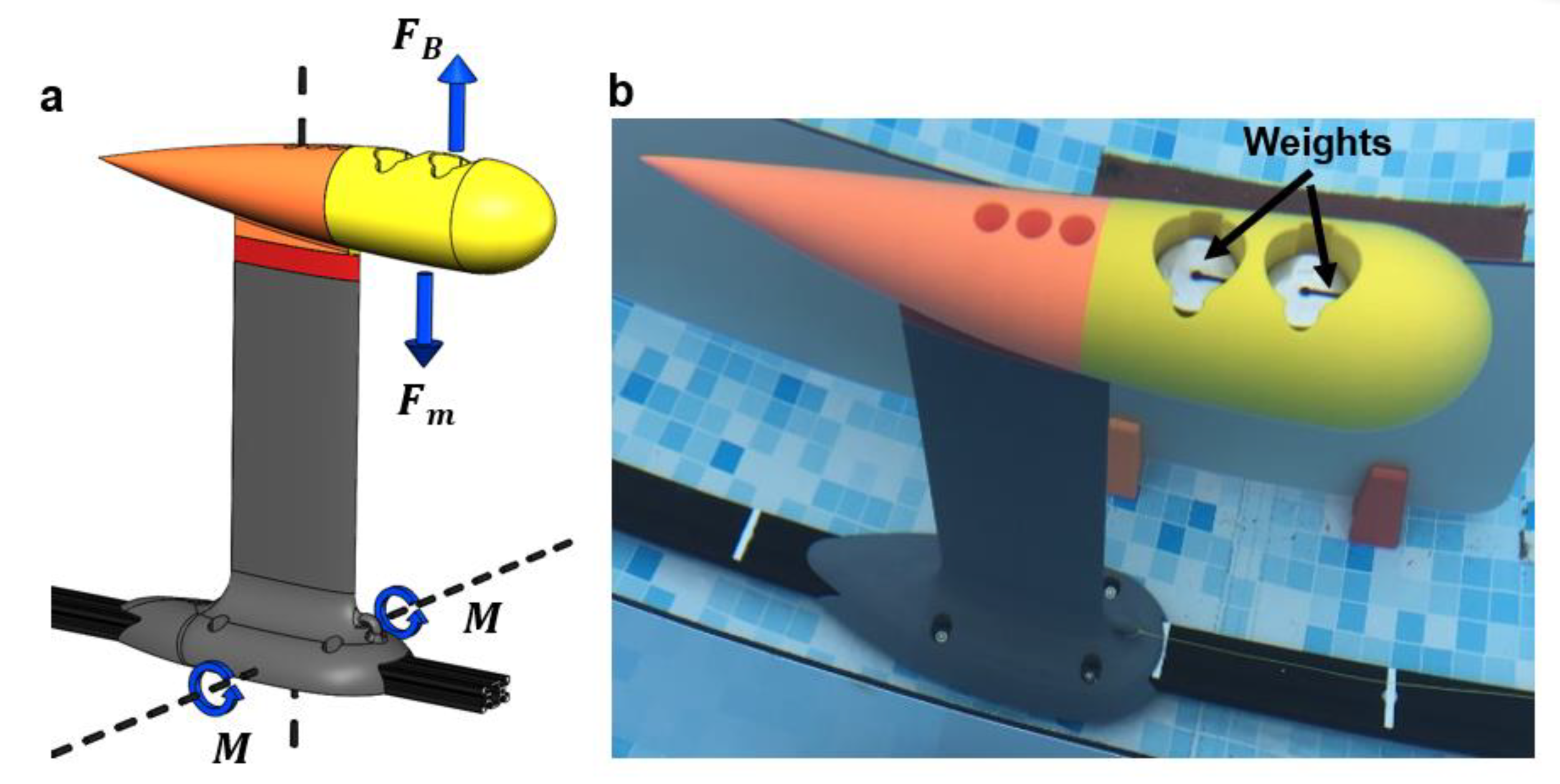
2.3. Test Rig Design and Manufacture

This section details the design to be manufactured of the test rig assembly, as displayed in Figure 2. The turtle chassis (head, carapace and rear flippers) was 3D-printed from PLA+ (Esun, Shenzhen, China) in six separate, hollow sections (Supplementary Figure S1). Each section was printed at 215 °C with 0.2 mm layer heights and with a consistent 1.6mm wall thickness. The part cooling fan was set to an 80% flow rate to capture fine details, but did not affect layer adhesion. Each part of the chassis was designed to fill with water through filling bungs at the bottom of each section to make the chassis slightly negatively buoyant. The front wings were manufactured in two sections: the wing tip to elbow section and elbow to shoulder section (Supplementary Figure S1). These used identical temperatures and layer heights as the chassis; however, 18 solid top and bottom layers with 9 shells at a 35% honeycomb infill were used for the wing tip to the elbow section. The shoulder to elbow section used the identical infill settings; however, 26 solid top and bottom layers were used with 13 shells. All parts were sliced using Simplify3D (Simplify3D version 4.1, Cincinnati, OH, U.S.A.) and printed on a “Caribou 420 MK3s Rel 3” machine (Caribou MK3s, Remagen, Germany). The printer was set up with a Mosquito Hotend, (Slice Engineering, Gainesville, FL, U.S.A.) with a 0.4 mm nozzle and dual-gear direct drive extruder (Bondtech, Värnamo, Sweden). Using these print settings, surface finishes of Ra 7 µm perpendicular to the flow direction and Ra 3 µm parallel to the flow direction were obtained. Surface roughness was measured with a stylus profilometer (FORMTALYSURF 50, Taylor Hobson, Leicester, U.K.) (Supplementary Figure S2). All fins were manufactured to 230 g with an identical volume of 226.5 cubic centimetres. The centre of buoyancy for every fin was 70 mm from the fin rotation axis, with the centre of mass located 73 mm from the rotation axis. This created a small torque to resist passive operation.

The pulley assembly was primarily 3D-printed, except for the linear rails, standard hardware and the main aluminium truss frame. All printed parts used Esun PLA+, except for the motor mount that was printed from PETG at 245 °C. PLA+ and PETG were printed with 4 shells, 8 top and bottom solid layers, with a 35% honeycomb infill.

To ensure the absolute lowest friction while running all rotating components, 100% Zirconia Oxide ceramic bearings were used, which also made sure the bearings that were located underwater did not suffer from corrosion. The motor and pulley assembly was installed onto a linear rail, allowing the motor and pulley to pull against the force sensor. The pulley cable was made from the Spectra fibre 50lb braided line (Spectra^®®, Honeywell, NC, U.S.A.) due to its high-strength and low-stretch properties. During towing, the braided line was designed to neatly wind onto the pully to ensure the system had a consistent velocity after the acceleration stage.

The pulley system was controlled by an electric circuit consisting of a stepper motor “NEMA 17”, an A4988 stepper motor driver (Allegro Microsystems, Manchester, NH, U.S.A.), a microcontroller (Arduino.cc, Somerville, MA, U.S.A.) and a variable D.C. power supply (SkyRC Technology, Guanlan, Shenzhen, China). The Arduino was used to control the angular speed of the motor in revolutions per minute (R.P.M.) using the A4988 driver. The necessary R.P.M. was calculated from the required linear velocity using the following formula: $RPM=\frac{60v}{2\pi r}$, where “$v$” is the linear velocity, and “$r$” is the radius of the pulley ($r$ = 0.0225 m). Furthermore, to ensure a smooth transition at the start of each test and to avoid high acceleration loads, linear velocity was defined as $v=0.2t$, where $t$, the time in second, was terminated at the maximum velocity to keep the system at the desired constant velocity. Moreover, to ensure smooth motor steps during the low initial speeds, micro-stepping of a ¼ step was implemented.

2.4. Testing Procedures

Drag force testing consisted of five procedures, all of which were repeated a minimum of five times at 0.6 m/s. The Arduino program that controlled motor speed was tuned to ensure motor speeds were within a 0.5% target. The speed was verified by timing how quickly the pylon passed white markers placed on the linear rail using high-speed video footage at 240 FPS. Additionally, the pully R.P.M. was verified with a digital tachometer to ensure the linear velocity was proportional to angular velocity values. All tests performed consisted of towing a pylon of a cross-section NACA 0010 on a linear rail, as seen in Figure 2, down a 4 m long, 2 m wide and 1m deep freshwater swimming pool at a temperature 20 to 21 °C. Data were collected for the last second of running to ensure the system was as close as possible to a steady-state. Depending on the test, the pylon would have the following items attached, consisting of:

-

Pylon only (no attachments);

-

Pylon with force sensitivity device (to measure system sensitivity to lift forces);

-

Pylon with sea turtle model and rigidly mounted wings (wings could not rotate);

-

Pylon with sea turtle model and passive wings (wings are free to rotate);

-

Pylon with sea turtle model with wings removed (no wings, turtle carapace only).

Running the pylon only without attachments resulted in a resistance of 0.596 ± 0.016 N at 0.6 m/s. This value was then subtracted from all force measurements. A sensitivity study was conducted to ensure that any lift forces generated did not affect the drag force due to an increase in load acting normal to the linear rail. This process involved designing the device, shown in Figure 4, that could retain a constant hydrodynamic drag force while controlling a variable force acting normal to the linear rail. Adjusting the normal force was achieved by inserting 100 g weights internally into the device (Figure 4b). The device produced a maximum buoyant force of 8.085 N, acting normal to the linear rail with no internal weights. Additionally, this buoyant force was positioned forward of the bearings to induce a moment to simulate the torque generated by the lift force from the rigid turtle wings. The findings from this exercise showed that the system’s sensitivity to forces acting normal to the linear rail could be neglected with changes only up to 0.06 N, as evident in the pull force data (Supplementary Figure S3).

The passively mounted wing and rigidly mounted wing both shared an identical geometry except for the attachment point, with the rigid wing using a splined input shaft to prevent rotation and the passive wing using a smooth input shaft running on ceramic bearings. This allowed the passive wing to freely rotate about the turtle’s shoulder during tow tests.

Upstroke angular displacement data were obtained by filming the turtle during a tow test from the front, as illustrated in Figure 5. Tests were performed at 0.6 m/s tow speeds. Filming was carried out with a Paralenz Vaquita camera (Paralenz, Rødovre, Denmark) at Full HD 240 FPS. The video footage was edited in the software “VideoPad Professional” (N.C.H. Software, Canberra, A.C.T., Australia) to find the time taken to complete the upstroke. The test rig was set up to release the fins at approximately 135° clockwise from the vertical axis, which was defined based on findings by van der Geest et al. [16] that were based on the position of the wing at the start of the upstroke in wild sea turtles. The top of the upstroke was taken as the wings highest point before leaving the camera frame. Based on the time taken for the wings to complete the angular displacement, angular velocity could be calculated for 0.6 m/s swim speeds.

2.5. Flow Pattern Generation

Dye injection was used to help better understand why the fluid dynamic forces changed for each testing case. Flow patterns generated by the turtle were documented by injecting a water-based dye. The water-based dye ensured it remained neutral after injection and did not sink or rise in the water column. Documentation of flow patterns was obtained by filming how the dye mixed with freshwater when the turtle passed through (Supplementary Figure S4a–d and Supplementary Video S1) using two high-speed cameras (Chronos 2.1-HD 32GB, Kron Technologies Inc, Burnaby, BC, Canada) filming at full HD 1000 FPS. Dye testing was utilised for this work due to its ease of application, low cost and due to it having been successfully applied in many high-level applications [24,25,26,27].

As no commercial devices were available to purchase for such a test, two devices were designed and built, shown in Figure 6a,b, to allow different methods of dye injection. Device one (Figure 6a) could inject significant levels of stationary dye with up to two colours. The device made it simple to acquire information on the wingtip vortex formation concerning passive and rigid wings. On the other hand, device two (Figure 6b) was designed to induce streamlines into the turtle’s incoming flow to help visualise flow separation and attachment (Supplementary Figure S4a–d and Supplementary Video S1). Both devices utilised medical syringes built into their central bodies and produced the dye injection via a hand trigger.

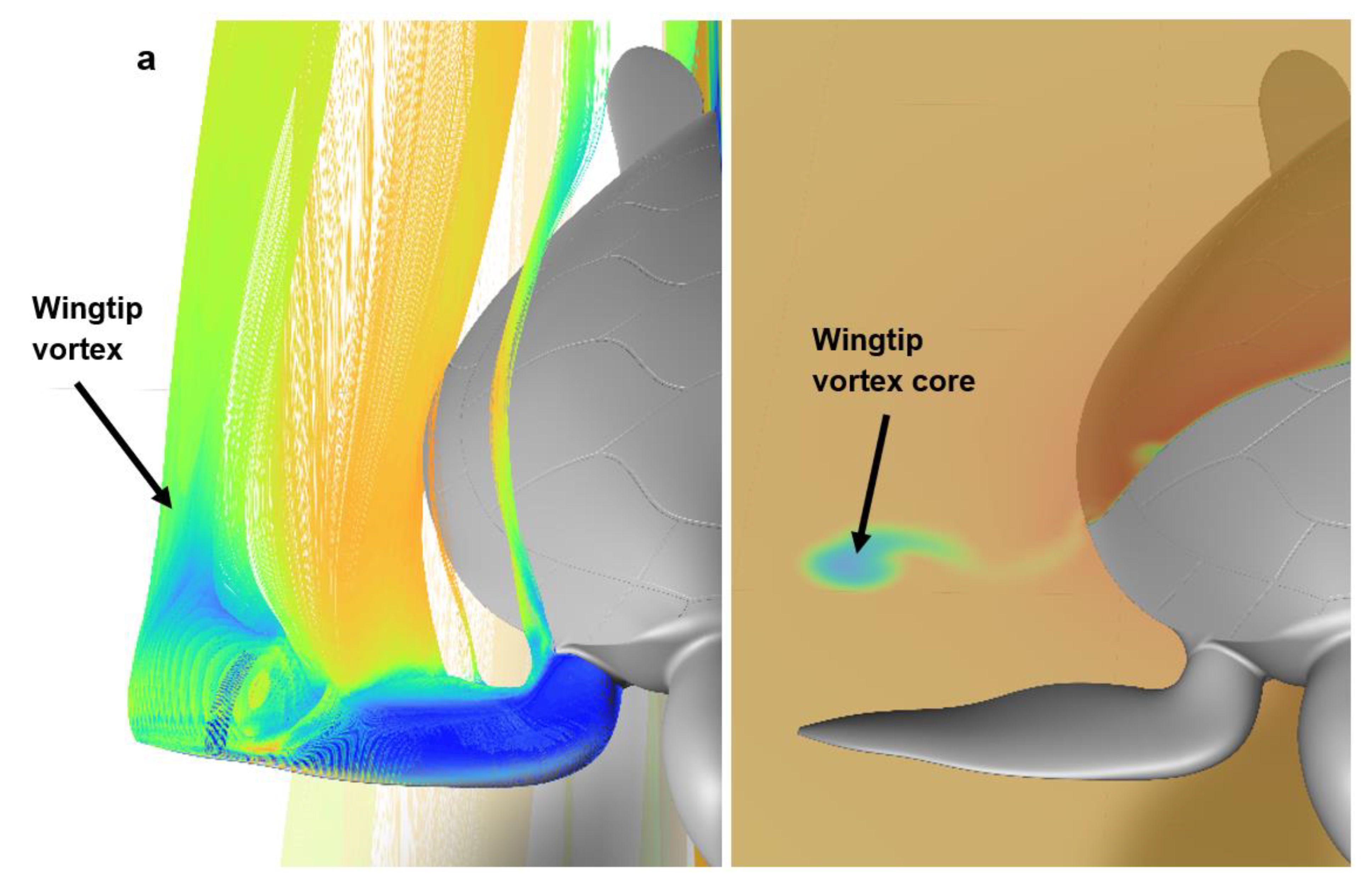
2.6. C.F.D. Analysis

C.F.D. simulations were produced with the commercial C.F.D. software ANSYS Fluent (ANSYS 2021 R2, Canonsburg, PA, U.S.A.) using the Reynolds average Navier–Stokes (RANS) models. The C.F.D. simulations in this study were only made for rigidly mounted wings. The simulations also served two purposes: firstly, to provide a second solution to the drag coefficients that did not rely on testing results, and secondly, to help display the flow features that caused the increase in drag during nonpassive wing operation.

The pylon geometry was subtracted from the computational domain and all surface fasteners to simplify the model, thus lowering the nodal count. The computational domain (Supplementary Figure S5a) was set up with a symmetry boundary condition to halve the domain and substantially lower computational expense. The curvature of the pool wall was modelled in and set as a zero-slip moving wall, with the pool surface modelled as a zero-shear/free-slip wall. All surfaces of the turtle geometry were set as zero-slip smooth walls, with the measured surface roughness not considered in any simulations. Fluents Poly-Hexcore mesh was used, containing approximately 12,500,000 nodes and 6,000,000 elements. Each simulation had an initial estimate using the realisable k-epsilon model before switching to the k-omega S.S.T. model. The mesh was refined down to an average wall $y^{+}$ value of 1.07 to resolve the flow down to the viscous sublayer. Bodies of influence were added at the wingtips, rear of the turtle’s body and one zone encasing the entire turtle assembly to refine the mesh in those critical areas. Monitors were set up to observe the scaled residuals, drag force, lift force, wall $y^{+}$ and the standard deviation of the velocity at the outlet. Comparing the C.F.D. values with field test values, a close correlation was achieved for the drag coefficient (Supplementary Figure S5b). Additionally, when comparing flow patterns from C.F.D. to field testing, corresponding flow feature trends were obtained.

3. Results and Discussion

This section is divided into three subsections. The first subsection describes the effect of a passive wing on the overall turtle drag coefficient ($c_d$), as well as detailing the contribution towards changes in $c_d$. Additionally, our turtle’s $c_d$ results and frontal area are compared with the same values from the literature to ensure the geometry correlates with previous works. The second subsection details the effects of the wing twist on the time required to complete the turtle’s upstroke. The final subsection details a numerical process to calculate the drop in swim speed due to the turtle producing a passive drag-reducing upstroke.

3.1. Effect of Passive Wings on the Turtle’s Drag Coefficient

Testing with the wings held rigidly would increase the drag force almost linearly for all values of wing twists. The contribution to the increase in drag came from an increase in magnitude of the wingtip vortex (Figure 7a) and increased flow separation due to adverse pressure gradients (Figure 7b) caused by the increase in wing twist. The passive wings (meaning the wing is free to rotate around its axes, referring to the axes of rotation in Figure 8d) were able to keep prolonged flow attachment (Supplementary Video S1 and Supplementary Figure S4), owing to the relative angle of attack remaining constant along the wingspan. This was due to the addition of an increasing vertical component of velocity towards the wingtip. Additionally, the wingtip vortex was cancelled out, likely due to the wing entering a near-equilibrium state, creating near-constant pressure across each surface and preventing any cross-flow due to pressure differences. To quantify these effects, the drag coefficient $(c_d$) was calculated by applying:

$$c_d=\frac{2F_d}{A_p{\rho }_{h2o}{v}^2}$$

(1)

where $F_d$ is the average drag force (obtained from test rig data) acting on the turtle and wing assembly, $A_p$ is the projected area perpendicular to the flow direction, ${\rho }_{h2o}$ is the fluid density and $v$ is the tow speed. All force measurements were taken at 0.6 m/s with a Reynolds number ($Re)$ of 297,970 based on the straight carapace length (S.C.L.). The Reynolds number was defined by:

$$Re=\frac{v{D}_{SCL}{\rho }_{h2o}}{{\mu }_{h2o}}$$

(2)

where $v$ is the tow speed, and the characteristic length is defined as $D_{SCL}$ with ${\rho }_{h2o}$ and ${\mu }_{h2o}$ being the fluid density and dynamic viscosity. Referring to Figure 8a, it can be observed that an average $c_d$ for a passive wing was 0.151 ± 0.008 and was obtained for all values of wing twist. Tests without wings produced a $c_d$ of 0.133 ± 0.012, which directly coincides with values obtained by T.Todd Jones et al. [28] of 0.13 ± 0.02 from castings (without front wings) of deceased green sea turtles through wind tunnel testing.

Additionally, the frontal area of our test rig model was between 0.0436 and 0.0482 m² (depending on wing twist). This closely correlates with findings by Kinoshita et al. [8] from 0.0416 to 0.0448 m² for similar-sized green sea turtles. Based on the mentioned literature, the accuracy of our green sea turtle geometry appears justified.

Based on the $c_d$ values, it can be observed that a passive wing, regardless of wing twist, only contributes to 12% of the overall drag on the turtle, whereas rigid wings contribute from 21% up to 50% of the overall drag depending on the value of wing twist.

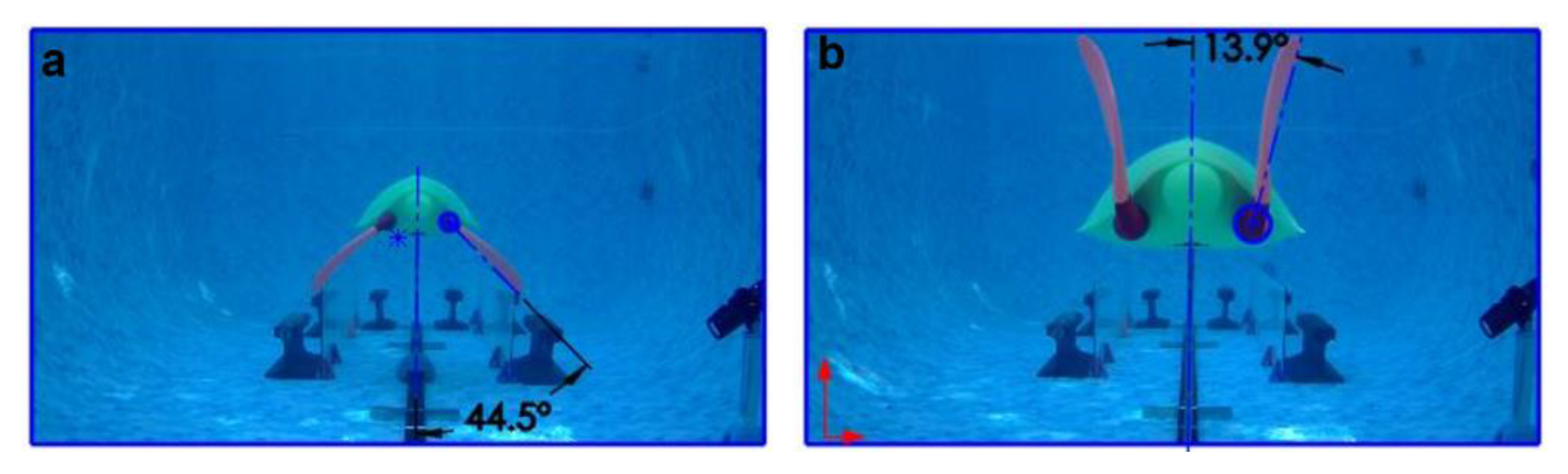
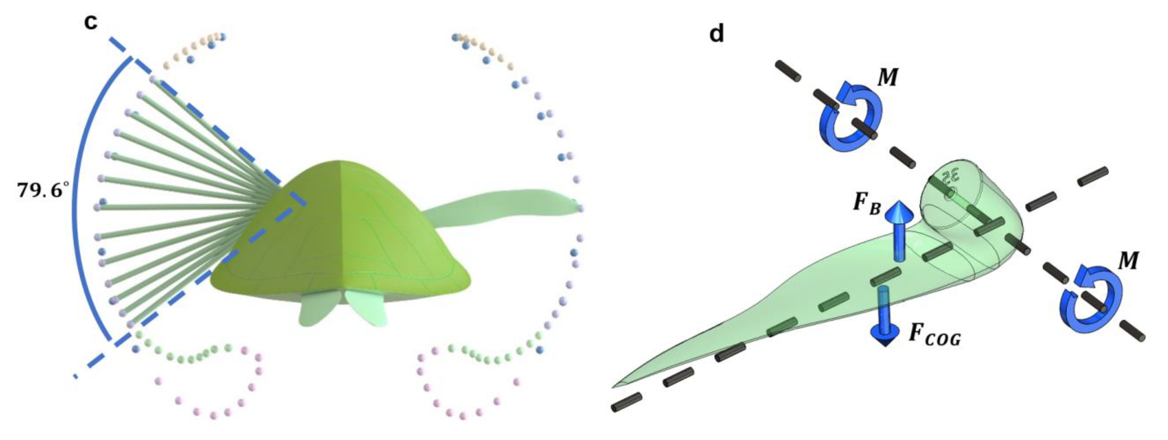
3.2. Passive Wing Rotation Speed Based on Wing Twist

Figure 8b displays the average angular velocity of a passive wing from the testing results at swim speeds of 0.6 m/s. Based on the average upstroke displacement of 79.6°, we found that a passive upstroke with a wing twist of 28° occurs in 1.25 s at a swim speed of 0.6 m/s, closely matching the findings of van der Geest et al. (Figure 8c) [16] of a 28° twist in 1.2 s. Moreover, this swim speed aligns neatly with the literature for the cruising speeds of sea turtles [22,23]. Unsurprisingly, the 35° wing twist produced the fasted upstroke at just 1.03 s, with the lowest wing twist of 10° completing the upstroke in 3.07 s.

Tests for this work were carried out with a slightly negatively buoyant wing geometry (Figure 8d). This was based on the body density of a sea turtle being 1046.5 kg/m³ [29] in saltwater of a density of 1025 kg/m³. There was a slight mismatch in the centre buoyancy compared with the centre of mass of the test wings due to manufacturing limitations; however, the position remained constant for all wings manufactured.

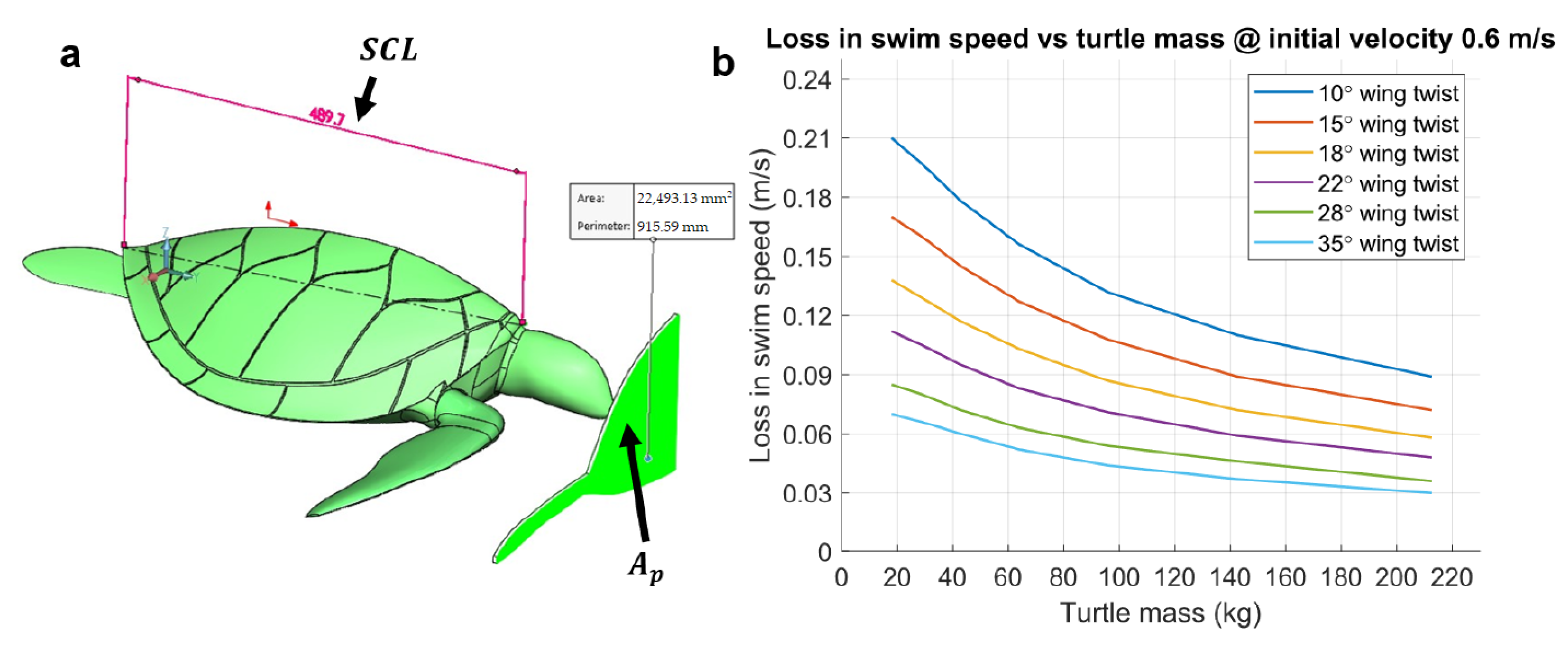
3.3. Velocity Drop during the Nonpropulsive Upstroke

Based on the findings, it is reasonable to assume the turtle does not generate any thrust during a passive upstroke, and thus, must lose swim speed during the upstroke period. To quantify this, the drop in swim speed as a function of time was derived from Newtonian physics as:

$$v_{drop}\left(t\right)=\frac{A_p{\rho }_{h2o}{v}^2{c}_d}{2m}t$$

(3)

where $v$ is the initial swim speed, $c_d$ is the average drag coefficient during the upstroke, ${\rho }_{h2o}$ is the fluid density and $t$ is the time taken for the upstroke to complete, with the turtle mass $m$ calculated based on research by Eguchi et al. [30], using their empirical function with respect to the S.C.L.: $m\left(SCL\right)=e^{0.96+0.04SCL}$. The frontal area $A_p$ was found by scaling the turtle CAD geometry, as seen in Figure 9a, within CAD to varying levels of the S.C.L. At each scale, $A_p$ was measured within CAD, as seen in Figure 9a. The results of $A_p$ with respect to the S.C.L. proved to align remarkably well with the past research values obtained by Kinoshita et al. [8].

It can be observed in Figure 9b that the loss in swim speed for larger turtles is as low as 0.03 m/s. Combining findings from earlier works that relate the mass and size of a turtle to its age [31,32] with findings from this study shows adult sea turtles > 80 kg are far less affected by swim speed losses generated by a passive upstroke than juveniles < 80 kg. This could suggest that adult green sea turtles are naturally more efficient swimmers. From an evolutionary and behavioural perspective, this suggestion makes sense, as the adult green sea turtles must undertake enormous migration distances during breeding seasons.

4. Conclusions and Future Work

Although in this study a rigid body with a constant wing twist is analysed, when applying a wing twist of 28°, our model completes the turtle’s upstroke in 1.25 s at a swim speed of 0.6 m/s. This aligns smartly with the findings of wild green sea turtles with a 28° wing twist completing their upstroke in 1.2 s [16] and a turtle swim speed of 0.6 m/s [22,23]. Additionally, this supports the work of van der Geest et al. [16] that found that the turtle’s wing remains relatively constant in shape during the upstroke. Based on these findings, we suggest that sea turtles apply a drag-reducing passive upstroke to conserve energy. This makes practical sense, as sea turtles have a cambered aerofoil-shaped wing that could generate inefficient thrust for the upstroke. The passive upstroke can be further justified because it occurs in approximately half the time of the turtle’s downstroke [14,16]. It must be noted that sea turtles may not always apply a passive upstroke. However, the passive upstroke can substantially lower the turtle’s drag coefficient to levels that cause minor changes in velocity during the upstroke period despite not generating any thrust force. This is particularly the case for larger turtles due to their increased body mass compared with their frontal area, potentially helping answer how green sea turtles (Chelonia mydas) migrate on such little energy intake [4,5,6,7]. With a passive upstroke, it is possible the turtle produces diminutive vortex shedding at the top of the upstroke, which could mean the reverse von Karman vortex is unattainable. To test that this hypothesis is accurate, the complete three-dimensional swimming routine will need to be reproduced. A dedicated work to produce this is currently being carried out, and the results will be disclosed in a future publication. Furthermore, this work provides new avenues to study animal locomotion without the need for animal interaction by utilising life-like additive-manufactured testing equipment coupled with simulation. Additionally, these findings could be optimised for conserving energy in bioinspired underwater drone technologies.

References

1. Hays, G.C.; Scott, R. Global patterns for upper ceilings on migration distance in sea turtles and comparisons with fish, birds and mammals. Funct. Ecol. 2013, 27, 748–756. [Google Scholar] [CrossRef]
2. Luschi, P.; Hays, G.C.; Del Seppia, C.; Marsh, R.; Papi, F. The navigational feats of green sea turtles migrating from Ascension Island investigated by satellite telemetry. Proc. R. Soc. Lond. Ser. B Biol. Sci. 1998, 265, 2279–2284. [Google Scholar] [CrossRef]
3. Wilme, L.; Waeber, P.O.; Ganzhorn, J.U. Marine turtles used to assist Austronesian sailors reaching new islands. C. R. Biol. 2016, 339, 78–82. [Google Scholar] [CrossRef]
4. Díaz-Abad, L.; Bacco-Mannina, N.; Madeira, F.M.; Neiva, J.; Aires, T.; Serrao, E.A.; Regalla, A.; Patrício, A.R.; Frade, P.R. eDNA metabarcoding for diet analyses of green sea turtles (Chelonia mydas). Mar. Biol. 2021, 169, 1–12. [Google Scholar] [CrossRef]
5. Howell, L.N.; Shaver, D.J. Foraging Habits of Green Sea Turtles (Chelonia mydas) in the Northwestern Gulf of Mexico. Front. Mar. Sci. 2021. Available online: https://www.frontiersin.org/articles/10.3389/fmars.2021.658368/full (accessed on 1 October 2022). [CrossRef]
6. Bjorndal, K.A. Nutritional Ecology of Sea Turtles. Copeia 1985, 1985, 736–751. [Google Scholar] [CrossRef]
7. McDermid, K.; Stuercke, B.; Balazs, G. Nutritional composition of marine plants in the diet of the green sea turtle (Chelonia mydas) in the Hawaiian Islands. Bull. Mar. Sci. 2007, 81, 55–71. [Google Scholar]
8. Kinoshita, C.; Fukuoka, T.; Narazaki, T.; Niizuma, Y.; Sato, K. Analysis of why sea turtles swim slowly: A metabolic and mechanical approach. J. Exp. Biol. 2021, 224, jeb236216. [Google Scholar] [CrossRef]
9. Chin, D.D.; Lentink, D. Birds repurpose the role of drag and lift to take off and land. Nat. Commun 2019, 10, 5354. [Google Scholar] [CrossRef] [Green Version]
10. Henningsson, P.; Hedenstrom, A.; Bomphrey, R.J. Efficiency of lift production in flapping and gliding flight of swifts. PLoS ONE 2014, 9, e90170. [Google Scholar] [CrossRef] [Green Version]
11. Iosilevskii, G. Centre-of-mass and minimal speed limits of the great hammerhead. R. Soc. Open Sci. 2020, 7, 200864. [Google Scholar] [CrossRef]
12. Hochscheid, S.; Bentivegna, F.; Speakman, J.R. The dual function of the lung in chelonian sea turtles: Buoyancy control and oxygen storage. J. Exp. Mar. Biol. Ecol. 2003, 297, 123–140. [Google Scholar] [CrossRef]
13. Davari, A.R. Wake structure and similar behavior of wake profiles downstream of a plunging airfoil. Chin. J. Aeronaut. 2017, 30, 1281–1293. [Google Scholar] [CrossRef]
14. Davenport, J.; Munks, S.A.; Oxford, P.J. A Comparison of the swimming of Marine and Freshwater Turtles. R. Soc. London. Ser. B Biol. Sci. 1984, 220, 447–475. [Google Scholar] [CrossRef]
15. Walker, W.F. Swimming in Sea Turtles of the Family Cheloniidae. Copeia 1971, 1971, 229. [Google Scholar] [CrossRef]
16. Van der Geest, N.; Garcia, L.; Nates, R.; Godoy, D.A. New insights into the swimming kinematics of wild Green sea turtles (Chelonia mydas). Sci. Rep. 2022, 12, 1–12. [Google Scholar] [CrossRef]
17. Izraelevitz, J.S.; Triantafyllou, M.S. Adding in-line motion and model-based optimisation offers exceptional force control authority in flapping foils. J. Fluid Mech. 2014, 742, 5–34. [Google Scholar] [CrossRef]
18. Licht, S.C.; Wibawa, M.S.; Hover, F.S.; Triantafyllou, M.S. In-line motion causes high thrust and efficiency in flapping foils that use power downstroke. J. Exp. Biol. 2010, 213, 63–71. [Google Scholar] [CrossRef] [Green Version]
19. Zhou, K.; Liu, J.-k.; Chen, W.-s. Numerical and experimental studies of hydrodynamics of flapping foils. J. Hydrodyn. 2018, 30, 258–266. [Google Scholar] [CrossRef]
20. Rivera, A.R.V.; Wyneken, J.; Blob, R.W. Forelimb kinematics and motor patterns of swimming loggerhead sea turtles (Caretta caretta): Are motor patterns conserved in the evolution of new locomotor strategies? J. Exp. Biol. 2011, 214, 3314–3323. [Google Scholar] [CrossRef] [Green Version]
21. Booth, D.T. Kinematics of swimming and thrust production during powerstroking bouts of the swim frenzy in green turtle hatchlings. Biol. Open 2014, 3, 887–894. [Google Scholar] [CrossRef]
22. Watanabe, Y.Y.; Sato, K.; Watanuki, Y.; Takahashi, A.; Mitani, Y.; Amano, M.; Aoki, K.; Narazaki, T.; Iwata, T.; Minamikawa, S.; et al. Scaling of swim speed in breath-hold divers. J. Anim. Ecol. 2011, 80, 57–68. [Google Scholar] [CrossRef]
23. Narazaki, T.; Sato, K.; Abernathy, K.J.; Marshall, G.J.; Miyazaki, N. Sea turtles compensate deflection of heading at the sea surface during directional travel. J. Exp. Biol. 2009, 212, 4019–4026. [Google Scholar] [CrossRef] [Green Version]
24. Bandyopadhyay, P.R.; Beal, D.N.; Hrubes, J.D.; Mangalam, A. Relationship of roll and pitch oscillations in a fin flapping at transitional to high Reynolds numbers. J. Fluid Mech. 2012, 702, 298–331. [Google Scholar] [CrossRef] [Green Version]
25. Carr, Z.R.; Chen, C.; Ringuette, M.J. Finite-span rotating wings: Three-dimensional vortex formation and variations with aspect ratio. Exp. Fluids 2013, 54, 1–26. [Google Scholar] [CrossRef]
26. Firat, E.; Ozkan, G.M.; Akilli, H. Flow past a hollow cylinder with two spanwise rows of holes. Exp. Fluids 2019, 60, 1–17. [Google Scholar] [CrossRef]
27. Kartheeswaran, A.; Jothi, T.J.S.; Arackal, R.S. Visualisation studies on plane jets at low Reynolds numbers. Sādhanā 2021, 46, 1–12. [Google Scholar] [CrossRef]
28. Todd Jones, T.; Van Houtan, K.S.; Bostrom, B.L.; Ostafichuk, P.; Mikkelsen, J.; Tezcan, E.; Carey, M.; Imlach, B.; Seminoff, J.A.; Rands, S. Calculating the ecological impacts of animal-borne instruments on aquatic organisms. Methods Ecol. Evol. 2013, 4, 1178–1186. [Google Scholar] [CrossRef]
29. Sato, K. Body temperature stability achieved by the large body mass of sea turtles. J. Exp. Biol. 2014, 217, 3607–3614. [Google Scholar] [CrossRef] [Green Version]
30. Eguchi, T.; Seminoff, J.A.; LeRoux, R.A.; Prosperi, D.; Dutton, D.L.; Dutton, P.H. Morphology and Growth Rates of the Green Sea Turtle (Chelonia mydas) in a Northern-most Temperate Foraging Ground. Herpetologica 2012, 68, 76–87. [Google Scholar] [CrossRef]
31. Chaloupka, M.; Limpus, C. Estimates of sex- and age-class-specific survival probabilities for a southern Great Barrier Reef green sea turtle population. Mar. Biol. 2004, 146, 1251–1261. [Google Scholar] [CrossRef]
32. Goshe, L.R.; Avens, L.; Scharf, F.S.; Southwood, A.L. Estimation of age at maturation and growth of Atlantic green turtles (Chelonia mydas) using skeletochronology. Mar. Biol. 2010, 157, 1725–1740. [Google Scholar] [CrossRef]
Figure 1. Three-dimensional model of a green sea turtle (Chelonia mydas) displaying various levels of wing twist of the pectoral wing. (a) Model showing upstroke with 28° degrees of wing twist. (b) Model showing downstroke with −72° of wing twist [16].
Jmse 10 01770 g001
Figure 2. Test rig assembly. (a) Complete test rig assembly CAD model, with a closeup of pully assembly shown at the top right. (b) The 3D-printed turtle with all wings. Yellow/red and orange/red = 35° twist, red = 28°, orange = 22°, green = 18°, yellow = 15° and blue = 10°. Passive wings are shown above turtle with rigid wings below. All wings are manufactured to the same volume and mass of 226.5 cubic centimetres and 230 g. (c) Image showing a typical test. (d) Workstation setup.
Jmse 10 01770 g002
Figure 3. Turtle geometry development. (a) Side, top and front view footage sets of wild green sea turtles (Chelonia mydas) overlayed in CAD, showing the two-dimensional sketches on each generated plane. (b) Images from van der Geest et al. [16] showing wing twist compared with CAD models during the upstroke. (c) Wing twist generation in CAD using the SolidWorks feature “Flex” to generate a linear varying twist between the plane at the wing tip (red plane) and elbow (green plane).
Jmse 10 01770 g003
Figure 4. Normal load sensitivity study. (a) Calibration device schematic with F B = 8.085 N and F m = 0.981 n , where n is equal to the number of 100 g weights used. (b) Calibration device with six 100 g weights installed.
Jmse 10 01770 g004
Figure 5. Upstroke data collection showing wings of 35° twist during a 0.6 m/s pull test. (a) Beginning of upstroke as wings leave the 135° constrainer. (b) Top of the upstroke measured anticlockwise from the vertical axis.
Jmse 10 01770 g005
Figure 6. The 3D-printed flow test equipment. (a) Dual-injection tool for inserting motionless clouds of dye. Actuation via hand trigger attached via a braided line to a sliding plunger. (b) Streamline injection tool to add streamlines of dye into turtle swim path. Actuation via hand trigger attached via a braided line to a rack and pinion mechanism (hand trigger location not in actual position).
Jmse 10 01770 g006
Figure 7. C.F.D. post-processing results of flow field velocity for a rigid wing of flex 35°. (a) Rigid wing generating the wingtip vortex. The image on the left shows streamlines starting at the turtle’s wing. The image on the right shows the vortex core via a transverse plane. (b) Longitudinal section plane through turtle wing showing flow separation due to adverse pressure gradients observed on rigid wings.
Jmse 10 01770 g007aJmse 10 01770 g007b
Figure 8. Testing data and parameters. (a) Drag coefficient vs. wing twist, the blue line represents a rigidly mounted wing with green line representing a passive wing. (b) Average upstroke angular velocity vs. wing twist for passive wings. (c) Sea turtle swimming pattern [16] detailing upstroke angular displacement of 79.6° for the turtle’s wing with solid green links and purple spheres. Blue spheres represent downstroke, pink spheres the sweep stroke, green spheres the recovery stroke one and orange spheres the recovery stroke two [16]. (d) Free body diagram of test rig fin showing the centre of gravity acting at 73 mm from the rotation axis and centre of buoyancy acting at 70 mm from the rotation axis.
Jmse 10 01770 g008aJmse 10 01770 g008b
Figure 9. Turtle geometry and its effects on swim speed. (a) Extraction of turtle frontal area A p with respect to S.C.L. from CAD. (b) Loss in turtle swim speed during a passive upstroke with an initial swim speed of 0.6 m/s versus turtle mass. Based on the time required for each wing to complete upstroke displacement of 79.6° obtained from testing data.
Jmse 10 01770 g009
Publisher’s Note: MDPI stays neutral with regard to jurisdictional claims in published maps and institutional affiliations.