Influence of Stern Rudder Type on Flow Noise of Underwater Vehicles

Abstract

The stern rudder of an underwater vehicle has a significant impact on the wake field and the flow noise. Hence, it is important to optimize the design of the stern rudder for reducing the radiated noise. In this work, a numerical model is set up to predict the flow noise of the underwater vehicle, based on the LES turbulence model and FW-H acoustic analogy method. After the verification study, the numerical prediction of the flow noise is compared with the experimental measurements to verify the accuracy of the numerical model. Then, the influence of sails on the flow noise is explored. It is observed that the existence of the sail significantly increases the noise at the low frequency. Furthermore, to examine the influence of the stern rudder type, the sound pressure levels of underwater vehicles with three full appendages having cross-type rudders, X-type rudders, and T-type rudders, are compared. The strong interaction between the sail’s wake and the stern rudder is evident. The underwater vehicle with T-type rudders exhibits the lowest sound pressure. In addition, the influence of the stern rudder type on the directivity of sound pressure levels is also presented.

1. Introduction

When an underwater vehicle travels below the surface of the sea, the stern rudders protruding from the main hull disturb the flow field, shed several vortices, and induce pressure pulsation and distribution on the vehicle surface. This phenomenon, in turn, affects the flow noise characteristics. A successful design requires an excellent main hull shape and appropriate stern rudder layout such that the designed underwater vehicle exhibits the characteristics of low resistance and low flow noise. Therefore, it is of great engineering significance to examine the influence of the stern rudder form on flow noise characteristics.

There are two main methods for studying the flow noise in underwater vehicles: experimental tests and numerical simulations. The main experimental tests include cavitation tunnel measurements, towed body measurements, and buoyant model experiments. Numerical prediction methods include direct numerical simulation (DNS) and hybrid numerical simulation. By directly solving the N-S equation, DNS is the most accurate method for obtaining the sound pressure pulsation of the flow field, but it requires excessively high computing resources and is not suitable for engineering calculations under complicated conditions. Using hybrid numerical simulation, the flow field is predicted first, and the far-field noise is obtained via acoustic analogy, which can ensure simulation accuracy and shorten the calculation time. Commonly used hybrid numerical simulation methods mainly include Reynolds average Navier-Stokes (RANS) random noise generation model [1,2,3], the turbulence model and acoustic analogy [4], the discrete vortex method and acoustic analogy [5], the vortex acoustic separation method [6,7], and other methods. The most widely used methods are the turbulence model and acoustic analogies.

To date, numerous numerical and experimental studies have been conducted on the flow noise of underwater vehicles. Huang et al. conducted numerical simulations of the flow noise of axisymmetric objects in a complex marine environment [8]. Luo et al. analyzed the radiated noise of an underwater jet propelled by a high-pressure water jet using a co-simulation method combining Computational Fluid Dynamics (CFD) and computational aeroacoustics. Combined with the k-ε turbulence model and Lighthill acoustic simulation, a water jet model for high-pressure water jet propulsion was established [9]. Zhang et al. examined and tested the flow noise around underwater axisymmetric models with a bio-inspired coating via a high-speed water tunnel experiment [10]. Wang et al. studied the mechanism and characteristics of the flow noise of underwater high-speed vehicles via experiments and simulation methods. The results showed that the flow noise of the target increases with an increase in the velocity, and the turbulent velocity and pulsating pressure are higher at the head of the model, followed by the tail. The convection noise contribution in the middle part was small [11]. Liu et al. carried out numerical simulation and experiments on a model-scale underwater vehicle to study the distribution characteristics and the generation mechanism of underwater vehicles flow noise [12].

The most widely used methods are the turbulence model and acoustic analogies. Wang et al. used large eddy simulation (LES) and Lighthill acoustic simulation methods to predict the hydrodynamic noise of an underwater vehicle. The variation characteristics along the axial and transverse directions, radiation directivity, and sound energy were investigated. Moreover, the hydrodynamic noise due to the sail and propeller was analyzed [13]. Yao et al. used the LES method to simulate the flow field around an underwater vehicle with full appendages and compared the flow noise predicted by the boundary element method and the Ffowcs Williams-Hawkings (FW-H) equation [14]. Duo Qu used LES, Lighthill acoustic simulation theory, and vibro-acoustic theory to numerically predict the flow and sound fields of the rudder at different rudder angles. Subsequently, the characteristics of hydrodynamic noise under hydrodynamic excitation, including flow noise and vibration acoustics, were analyzed [15]. Based on the Volume of Fluid (VOF) multiphase flow and the Schnerr and Sauer cavitation models, Tu et al. established an LES/FW-H coupled numerical model to simulate the noise characteristics of underwater high-speed vehicles and combined it with a water tunnel experiment to examine those noise characteristics under different operating conditions [16]. SEZEN S et al. used RANS and Detached-Eddy Simulation (DES) solvers, combined with the porous FW-H (P-FWH) equation, to predict the hydrodynamic and underwater acoustic performance of a marine propeller in open water [17]. HU J et al. predicted contra-rotating propeller noise using the shear stress-transfer k-ω turbulence model, FW-H acoustic model, and the Schnerr-Sauer cavitation model [18]. Kolahan et al. used the LES turbulence approach and Sauer mass transfer models to analyze the cavitation phenomenon around the sphere in different cavitation numbers [19]. Pendar M.R et al. used the LES model to investigate the impact of using wavy leading-edge (WLE) airfoils in combination with curved multidielectric barrier discharge (DBD) plasma actuators as hybrid passive and active flow control mechanisms [20,21].

However, there is a paucity of studies on the influence of stern rudders on the flow noise characteristics of underwater vehicles. Shi Yao et al. conducted a numerical simulation of the flow field and flow noise on SUBOFF using the Lighthill acoustic simulation and the LES method. It was determined that the noise of X-type rudders was 3 dB less than that of cross-type rudders [22]. Zhang et al. predicted the flow field and flow noise of an underwater vehicle using the Lighthill acoustic simulation theory and FW-H equation, and they studied the influence of the stern rudder on the flow noise. The resistance and flow noise of the cross-type and X-type rudders were simulated. The results showed that the X-type rudders have a weaker blocking effect on the flow field than traditional cross-type rudders, and the flow noise of the X-type stern rudders is improved to a certain extent [23]. Xiao et al. conducted numerical simulations on an underwater vehicle with X-type stern rudders to examine the influence of different rudder areas on the resistance and wake field [24]. Jeon M. et al. evaluated the hydrodynamic performance of +rudder and ×rudder submarines during environmental disturbances. The study shows that the ×rudder submarine with improved control force has an advantage in maneuverability [25].

Current studies mainly focus on the influence of the vehicle hull on the flow noise, particularly the head shape. However, there is a lack of comprehensive and systematic investigation of the effect of stern rudder on the flow noise. To comprehensively examine the influence of the stern rudder arrangement on the noise level of underwater vehicles, the effectiveness of the LES turbulence model, combined with the FW-H equation, in predicting flow noise was verified by comparing the numerical predictions with the experimental measurements of the flow noise of an Albacore underwater vehicle. Subsequently, the influence of the sail on the flow field and the flow noise was investigated based on the validated numerical model. Finally, the flow field and flow noise characteristics of three full-appendage vehicles with different stern rudders were compared. The strong interaction between the sail’s wake and the stern rudder is evident. The flow noise contribution of the stern rudders and their rudder surfaces were calculated, and a stern rudder layout with low flow noise was obtained. In this study, we provide insights into the design of the overall layout of underwater vehicles.

2. Numerical Approach

2.1. Large Eddy Simulation(LES)

The flow field of an underwater vehicle is generally in a uniform flow state, and the speed of the underwater vehicle is normally in the range of 1.03 m/s–6.17 m/s (2 kn–12 kn). Therefore, the flow-field control equation can use the continuity and momentum equations of an incompressible fluid as follows:

$$\frac{\partial u_i}{\partial x_i}=0$$

(1)

$$\frac{\partial \rho u_i}{\partial t}+\frac{\partial \rho u_i{u}_j}{\partial x_j}=-\frac{\partial P}{\partial x_i}+\mu \frac{{\partial }^2{u}_i}{\partial x_j\partial x_j}$$

(2)

where P denotes pressure, ρ denotes fluid density, u denotes velocity vector, μ denotes the dynamic viscosity coefficient, and i and j denote the components of the ith and jth directions of the variable, respectively.

In the LES model, vortices are classified into two parts based on the scale of the eddy: large- and small-scale eddies. Large scale eddies are solved directly, whereas the influence of small eddies is simulated. This implies that the solution variable is decomposed into large-scale and small-scale vortices:

$$u_i=\widehat{u_i}+u_i^{\prime }$$

(3)

The subgrid turbulent viscosity of the LES turbulence model is simulated using the Wall-Adapting Local-Eddy (WALE), which is used to characterize the effect of small-scale vortices on the flow. The WALE viscosity is the most widely used sublattice model for characterizing turbulent viscosity:

$${\mu }_t=\rho {\Delta }^2{S}_W$$

(4)

where Δ denotes the turbulence length scale or mesh filter width and S_W denotes the deformation parameter.

$$\Delta =\{\begin{array}{c}{C}_W{V}^{1/3}\\ \min \left(\kappa d,C_W{V}^{1/3}\right)\end{array}$$

(5)

$$S_W=\frac{S_d:S_d^{3/2}}{S_d:S_d^{5/4}+S:S^{5/2}}$$

(6)

$$S_d=\frac{1}{2}\left[\nabla \mathrm{u}·\nabla \mathrm{u}+{\left(\nabla \mathrm{u}·\nabla \mathrm{u}\right)}^T\right]-\frac{1}{3}tr\left(\nabla \mathrm{u}·\nabla \mathrm{u}\right)I$$

(7)

where C_W = 0.544, κ = 0.41.

The RANS turbulence model applies the statistical theory to average the unsteady Navier-Stokes equation between time intervals to solve the time mean required in engineering. It has low grid requirements and fast calculation speed, which is suitable for engineering applications. DES turbulence model implements the RANS model in the area near the wall, and the LES model in the area far away from the wall. It can solve large separation flows in areas far from the wall, while significantly reducing the amount of mesh compared to the LES. Thus, the computation efficiency of the DES model is higher than the LES model, while the LES model provides more details on the flow field and pressure distribution. Their performance on the prediction of the flow noise will be shown in the Verification and Validation section.

2.2. FW-H Acoustic Analogy Method

The numerical study of flow noise is commenced with the Lighthill acoustic analogy theory. The Lighthill equations are derived from Navier-Stokes (NS) equations of fluid mechanics [26,27]. In recent years, the FW-H equation, developed from the Lighthill equation, has been used to predict flow noise [28].

The FW-H equation is proposed to solve the sound problem of free-moving objects in fluids [28], which is expressed as follows:

$$\left(\frac{{\partial }^2}{\partial t^2}-c^2\frac{{\partial }^2}{\partial y_i^2}\right)\left(\overline{\rho -{\rho }_0}\right)=\frac{{\partial }^2\overline{T_{ij}}}{\partial y_i\partial y_j}-\frac{\partial }{\partial y_i}\left(p_{ij}\delta \left(f\right)\frac{\partial \left(f\right)}{\partial y_j}\right)+\frac{\partial }{\partial t}\left({\rho }_0{v}_i\delta \left(f\right)\frac{\partial f}{\partial y_i}\right)$$

(8)

where $\overline{\rho -{\rho }_0}$ denotes the generalized density perturbation, $\overline{T_{ij}}$ denotes the generalized function equaling to Lighthill’s stress tensor. The symbol $p_{ij}$ can be reinterpreted as the difference of stress tensor from its mean value. $f=0$ represents the surface S, $f>0$ is outside any surfaces, $f<0$ means within them. $\delta$ is the one-dimensional delta function.

The aforementioned equation is the FW-H equation, and its solution is expressed as follows:

$$4\pi c^2\left(\rho \left(y,t\right)-{\rho }_0\right)=\frac{{\partial }^2}{\partial y_i{y}_j}{{\displaystyle \int }}^{ }\left[\frac{T_{ij}J}{r\left|1-M_r\right|}\right]d\eta -\frac{\partial }{\partial y_i}{{\displaystyle \int }}^{ }\left[\frac{p_{ij}{n}_{j}A}{r\left|1-M_r\right|}\right]dS\left(\eta \right)+\frac{\partial }{\partial t}{{\displaystyle \int }}^{ }\left[\frac{{\rho }_0{v}_n}{r\left|1-M_r\right|}\right]dS\left(\eta \right)$$

(9)

where η denotes the Lagrangian coordinate system moving at the same speed as the moving wall (body coordinate system), cM denotes the convective velocity of the source term. $y=\eta +{\int }_{}^{\tau }cM\left(\eta ,{\tau }^{\prime }\right)d{\tau }^{\prime }$, where M_r denotes components of M in the r-direction. $r=\left|x-y\right|$, where x denotes field point and y denotes source point. Furthermore, J denotes Jacobian transformation matrix as follows:

$$J=\exp \left\{{{\displaystyle \int }}_{}^{\tau }divcM\left(\eta ,{\tau }^{\prime }\right)d{\tau }^{\prime }\right\}, A=J\left|gra{d}_{y}f\right|{\left|gra{d}_{\eta }f\right|}^{-1}$$

(10)

3. Verification and Validation

An Albacore underwater vehicle model was used to verify the numerical simulation method. The geometric size of the vehicle is shown in Figure 1, with a length of 3.2 m and maximum diameter of 0.4 m. A realizable K-ε two-layer model was used to calculate the steady flow field. The number of iterative steps was set to 2000. Considering the results of the steady simulation as initial conditions, the unsteady simulation of the flow noise was solved using the LES and the FW-H models. The number of internal iterations was selected as five, and the time step was set to 0.0001 s. When the simulation tended to be stable, 0.5 s of the simulation were selected as the result. Then, the simulation results of the underwater flow noise of Albacore were compared with the experimental measurements reported by Zhang Huaixin in the circulating water tunnel of CSSRC [29] to verify the accuracy of the numerical method in predicting flow noise in this study.

The boundary conditions of the computational domain are shown in Figure 2. The distance between the velocity inlet and underwater vehicle model was the vehicle length, and the pressure outlet for the underwater vehicle model was twice that of the vehicle length. The four sides of the computational domains were set as the plane of symmetry, and the distance between the sides of the underwater vehicle model was five times the vehicle diameter.

Space discretization was performed using the trimmed mesh, and the normal thickness of the first-layer mesh satisfied y + < 1. The mesh distribution in the longitudinal section is shown in Figure 3.

The simulation results of the mesh independence verification and time-step independence are shown in Figure 4 and Figure 5, respectively. Four groups of meshes were obtained by changing the size of the base meshes to $\sqrt{2}$. The relative difference value D represents the relative size of the resistance coefficient of different mesh numbers and maximum mesh numbers D = (𝐶 − 𝐶_𝑚𝑎𝑥)/𝐶_𝑚𝑎𝑥 × 100%. Compared with 7.53 million meshes, when the number of meshes is 4.5 million, there is no significant difference in the resistance coefficient. Considering the simulation accuracy and cost comprehensively, 4.5 million meshes were selected for subsequent calculation. Different time steps were considered to calculate the resistance, and the results did not change significantly. Finally, a time step of 1 × 10 s was selected for subsequent calculations.

The SPL formula is applied to analyze the sound pressure levels at different frequencies.

$$SPL=20\log \left(\frac{p}{p_0}\right)$$

(11)

where p is the pressure value after Fourier transform processing, and p₀ is the reference sound pressure value, which is taken as $1\times {10}^{-6}$ Pa in water. Then, the total sound pressure level integrates the sound pressure levels of different frequency and can represent the magnitude of flow noise in the whole frequency range. The formula is as follow:

$$OSPL=10lg\left({10}^{0.1SP{L}_1}+{10}^{0.1SP{L}_2}+\cdots +{10}^{0.1SP{L}_n}\right)$$

(12)

where $SP{L}_1,SP{L}_2,\cdots ,SP{L}_n$ are the sound pressure levels in the range from 0 Hz to 5000 Hz.

For the noise prediction of the Albacore underwater vehicle, there is no single-stage sub-source because the vehicle surface exhibits no movement. Hence, this belongs to the noise problem of the static wall surface. Only the noise generated by the dipole source was calculated by the FW-H model. The predicted sound pressure level spectra of points A and B inside and outside the underwater vehicle, respectively, are shown in Figure 6. The numerical predictions matched well with the experimental values in the range of 500–5000 Hz, which verifies the accuracy of the proposed model.

In this study, to demonstrate the influence of the turbulence model on the flow noise prediction, the detached-eddy simulation (DES) model and SST k-ω model were adopted to simulate the same scenario as the LES model using the same mesh and time step. The flow noise prediction using the FW-H model is shown in Figure 6.

It is found that the LES turbulence model provides accurate predictions in terms of the sound pressure and is suitable for the prediction of the underwater vehicle flow noise. However, the modelling method of the LES turbulence model requires fine meshes to achieve high accuracy, and its computation is much more time-consuming than RANS and DES models. Currently, using the proposed numerical model to predict the flow noise of the full-scale underwater vehicle is very computational expensive and is impossible to be applied for engineering applications, since it requires fine mesh and small time steps.

The enormous difference between the green and black curve is also evident in Figure 6. When the DES turbulence model is applied to simulate the flow field near the body surface, the RANS turbulence model is actually used. Correspondingly, the fluctuation of the hydrodynamic pressure on the body surface is significantly under predicted because of the Reynolds-Averaged treatment of the RANS turbulence model. The sound pressure level predicted by the FW-H model is depending on this fluctuation of the hydrodynamic pressure. Therefore, the LES model and the DES model provides very different results, as shown in Figure 6. Meanwhile, the difference of the predictions between the DES model and RANS model are quite small, because the fluctuation of the hydrodynamic pressure on the body surface are both predicted by RANS turbulence model. It is worth mentioning that the mesh and the time step used for the three turbulence models in this study are the same. The comparison verified the effectiveness of the set-up of the LES and FW-H models.

4. Influence of Sail on Flow Noise

It is important to check whether the flow cavitation occurs when the flow noise is predicted. The cavitation’s occurrence is usually characterized by the cavitation number, which is defined as:

$$\sigma =\frac{p_{\infty }-p_v}{1/2\rho v_{\infty }^2}$$

(13)

where p_∞ and v_∞ are the absolute pressure and velocity of the selected point in the flow field; p_v is the saturated vapor pressure at a certain temperature; ρ is the liquid density. Normally, when the cavitation number is under the value of 1, the cavitation should be considered. In this work, the minimum value of the cavitation number was 5, based on the simulated flow field. Therefore, the cavitation model is not applied in the numerical model.

An Albacore underwater vehicle was used as the hull shape, and an upright sail was added to explore the influence of the sail on flow noise. The incoming flow velocity was 3.56 m/s. The geometric shape of the hull is illustrated in Figure 7. The sail position was 0.896 m behind the stagnation point of the hull’s leading edge, length of the sail was 0.386 m, and the top of the sail was 0.4 m away from the central axis.

It can be observed from the velocity field in Figure 8, surface pressure in Figure 9, and Q-contour in Figure 10, that the existence of the sail disturbs the flow field around the underwater vehicle. With large changes in velocity and pressure occurring at the front and back edges of the sail, a large disturbance occurs at the rear of the sail, resulting in vortices flowing backward along the hull.

The FW-H model was used to calculate the flow noise of the smooth underwater vehicle and vehicle hull with a sail. By considering the vehicle center as the center of the circle of monitoring points and a radius of 20 m, 36 sound pressure monitoring points were set-up on the transverse cross section, middle longitudinal section, and horizontal section. The arrangement of the monitoring points in the longitudinal section is shown in Figure 11.

All the sound pressure level results in this study were converted to equivalent values at the 1-m position. A comparison of the flow noise in all directions between the underwater vehicle with a sail and hull without a sail is shown in Figure 12. Given the existence of sails, the flow noise distribution of the two hulls obviously differs in terms of the transverse cross section. The noise pressure levels on the left and right sides of the underwater vehicle with a sail significantly increase, but not in the upper and lower directions because the projected area of the sail on the side is larger than that in the length direction. The influence of sail flow noise on the lateral direction is greater than that on the length direction, resulting in a noncircular distribution of flow noise in the transverse cross section. As shown in the noise directivity of the horizontal section, the existence of the sail significantly increases the sound pressure levels in the horizontal section, and the sound pressure levels increase by 9–15 dB.

Figure 13 shows the sound pressure level spectrum of the underwater vehicle with sail and hull without sail at the SZ9 monitoring point. The sound pressure level of the underwater vehicle with sail was larger than that of only hull in the whole frequency range, and it was significantly larger than that of only hull in the range of 0–60 Hz. This indicated that the noise generated by the sail is concentrated in the low frequency. The total sound pressure level of only hull at the monitoring point was 77.48 dB and that of the vehicle with sail was 88.24 dB. The increase in sound pressure level was 10.76 dB. The low frequency sound pressure is induced by the vortex shedding of the sail at the trailing edge. For the bare hull case, the flow separation around hull is not significant, and the size of the generated vortices are small. The corresponding radiated sound pressure level in the frequency range of 0–60 Hz is not high. However, for the case with the sail, the large amount of vortex shedding induced by the appendage, as shown in Figure 10, dominates the low frequency sound pressure, and the big difference shows up in the low frequency range.

5. Influence of Stern Rudders on the Flow Noise

5.1. Flow Field Simulation Results

Cross-type, X-type, and T-type rudders were added to an underwater vehicle with a sail to investigate the influence of the stern rudder on convective noise. The geometric model is illustrated in Figure 14. The profile shape of the stern rudders was NACA0012, and cross-type rudders and X-type rudders had four rudders. The top of the stern rudder was 0.2 m away from the central axis, the top chord length of the stern rudder was 0.12 m, and the bottom chord length of the central axis was 0.230 m. The stern rudder was positioned 0.168 m ahead of the aft stagnation point of the hull. T-type rudders had only three wings. Although the upper cross-type rudder was cancelled, the area of the horizontal rudders and lower rudder increased such that the total rudder area was the same for the cross-type rudders and X-type rudders.

In Figure 15, it can be observed from the longitudinal section velocity field that there is a large disturbance behind the sail, and the vortex shed from the sail influences the upper stern rudder. Figure 16 shows that the upper rudder of the cross-type rudders is just in the vortex shedding caused by the sail, which increases the pressure pulsation on the surface of the rudder and adversely affects the noise. The X-type rudders were deflected to a certain angle, which can reduce the adverse effects of vortex shedding of the sail. However, the two upper rudders of the X-type rudders were still disturbed by vortex shedding. The T-type rudders were least affected because the layout style had no upper rudder, and the two horizontal rudders were far from vortex shedding.

5.2. Simulation Results of Flow Noise of Underwater Vehicle with Full Appendages

The flow noise of the full-appendage underwater vehicle with different rudder layouts was calculated. The sound pressure monitoring points at SZ9 were considered as the characteristic points, and the sound pressure level spectrum was analyzed. The results are shown in Figure 17. It can be observed from the figure that the peak frequency of the sound pressure level is concentrated in the low frequency range of 0–100 Hz. Another peak frequency appears in the range of 460–530 Hz, which is the same as the peak frequency of the flow noise of the underwater vehicle without a sail and rudder. This indicates that the peak frequency of the flow noise generated by the vehicle hull is within this range. The peak at the lower frequency is due to the presence of the stern rudder. This viewpoint is explained in subsequent simulation results. The total sound pressure levels of the underwater vehicles with three full appendages and different rudder layouts at the monitoring point were 94.50 dB for cross-type rudders, 93.39 dB for X-type rudders, and 92.27 dB for T-type rudders. The values of peak sound pressure level and total sound pressure level were as follows: cross-type rudders > X-type rudders > T-type rudders.

The flow noise results for all the directions are presented in Figure 18. In the transverse cross section, the noise of T-type rudders is less than that of cross-type rudders and X-type rudders in all directions. Although cross-type rudders and X-type rudders are symmetrical structures, there are significant differences in the noise directivity between them on the transverse cross section. The rudder of cross-type rudders is affected by the sail vortex shedding, which increases the pressure pulsation on the surface of the rudder. Hence, the sound pressure levels in the left and right directions of the cross-type rudders are significantly greater than those in the upper and lower directions. The 45-° arrangement of the X-type rudders prevents the influence of sail vortex shedding to a certain extent. However, given that two rudders experience interference, the transverse cross-sectional directivity becomes circular. In addition, it is found that the x rudders radiate more energy in the directions of 90 degrees and 270 degrees than the other two. This phenomenon is compatible with the expectation.

According to the directivity diagram of the transverse cross section directivity, there is an obvious relationship between the flow noise sound pressure level of the three different types, namely, X-type rudders > cross-type rudders > T-type rudders. According to the directional diagram of the longitudinal and horizontal sections, the relationship of the flow noise sound pressure level of the three different types of rudders is as follows: cross-type rudders > X-type rudders > T-type rudders.

To quantitatively represent the overall flow noise, the sound energy of 108 monitoring points in the transverse, longitudinal, and horizontal sections are averaged to calculate the total sound pressure levels of underwater vehicles with different stern rudder types, as shown in Figure 19. Based on the total sound pressure level, namely cross-type rudders > X-type rudders > T-type rudders, it was observed that the sail has an impact on the noise of the stern rudder part, and thereby, reduction in the impact reduces the flow noise.

5.3. Simulation Results of Flow Noise at Stern Rudders

The FW-H equation was applied to the surface of the stern rudder separately to calculate the flow noise radiation of the stern rudder. Specifically, 32 noise monitoring points are established in the transverse cross section of the one-third chord length of the stern rudder as shown in Figure 20. The sound pressure levels of the different stern rudder types are shown in Figure 21. The noise generated by the cross-type rudders is larger in the left and right directions, that of the X-type rudders is more evenly distributed in all directions, and the noise generated by the T-type is larger in the upper and lower directions. Based on the overall sound pressure level, cross-type rudders > X-type rudders > T-type rudders.

The radiation sound pressure level spectrum of the stern rudder at WY0 monitoring points is shown in Figure 22, and the peak frequency appears in the range of 0–100 Hz. Given that the integral surface calculated in this section was only the surface of the stern rudder, it can be determined that the noise at this frequency was generated by the stern rudders, which is consistent with the previous judgment. Based on the peak sound pressure level value, noise of the cross-type rudders was 76.34 dB, noise of the X-type rudders was 72.91 dB, and noise of the T-type rudders was 60.73 dB, indicating that the pulsating pressure on the surface of the cross-type rudders is greater than those on X-type rudders and T-type rudders. The T-type rudders were least affected by sail vortex shedding, and the noise level was the lowest because of the cancellation of the upper rudder.

Each single rudder of each rudder type was calculated, and the influence of a single rudder on the flow noise was obtained. The flow noise of each type of rudder is shown in Figure 23, Figure 24 and Figure 25. The upper rudder of the cross-type rudders exhibited the highest flow noise with a maximum sound pressure level of 86.28 dB. However, the left and lower rudders exhibited 80.02 dB and 78.30 dB, respectively. This was mainly due to the vortex shed by the sail entering the wake field and intensifying the pressure pulsation on the upper rudder surface. This in turn adversely affected the flow noise of the upper rudder. The upper-left rudder of the X-type rudders was also affected by the vortices of the sail. The noise generated by the upper-left rudder was greater than that generated by the lower-left rudder, and the maximum pressure levels were 81.42 dB and 79.71 dB, respectively. The left rudder and lower rudder of T-type rudders were less affected by the vortex, and the maximum noise pressure levels were 79.89 dB and 80.65 dB, respectively.

6. Conclusions

In this study, the flow noise characteristics of an underwater vehicle were calculated and analyzed based on the LES model and the FW-H method. The characteristics of the flow noise of an underwater vehicle with a sail and a vehicle without a sail were compared, and the effects of three different stern rudder types on the flow noise of an underwater vehicle with full appendages were investigated.

• The results of the flow noise simulation of an underwater vehicle with a sail showed that the existence of a sail significantly increases the sound energy in the horizontal section, and the sound pressure level increases by 10–15 dB.
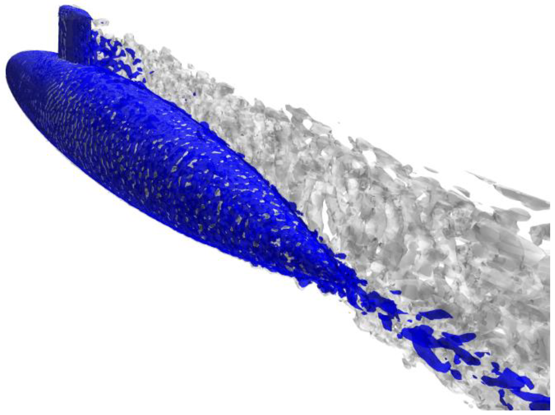
• The velocity fields and Q-contour figures of different stern rudder types showed that the stern rudders were observed in the disturbance generated by the sail. The degree of impact was as follows: cross-type rudders is greater than X-type rudders, and X-type is greater than T-type rudders.
• The flow noise simulation results showed that the sound pressure level of the flow noise was also larger for the stern rudder types, which were heavily influenced by sail vortex shedding. This was evident from the sound pressure level directivity of the three sections and sound pressure level of all monitoring points. The relationship of sound pressure level of the three types of stern rudders was as follows: cross-type rudders is greater than X-type rudders, and X-type is greater than T-type rudders.
• The flow noise simulation results for each single rudder surface showed that the sound pressure level of the upper rudder of the cross-type rudder was significantly larger than that of the lower rudder and left rudder. The sound pressure level of the upper left rudder of the X-type rudder was significantly higher than that of the lower left rudder. Furthermore, T-type rudders exhibited lower sound pressure levels on the left and lower rudders. The results showed that X-type rudders, particularly T-type rudders, could significantly reduce the sound pressure level of stern rudder noise.
• The noise frequencies generated by the sail and stern rudders were mainly concentrated at low frequencies, whereas the peak frequency of the noise generated by the vehicle body was mainly in the middle frequency.

The current work is conducted by using the model-scale underwater vehicle. In the future, the influence of stern rudder type on the flow noise of the underwater vehicle with different scales will be investigated. In addition, the propeller will be added into the numerical model, and the influence of stern rudder type on the propeller noise will be examined.

References

1. Bechara, W.; Bailly, C.; Lafon, P.; Candel, S.M. Stochastic approach to noise modeling for free turbulent flows. AIAA J. 1994, 32, 455–463. [Google Scholar] [CrossRef] [Green Version]
2. Ewert, R. Broadband slat noise prediction based on CAA and stochastic sound sources from a fast random particle-mesh (RPM) method. Comput. Fluids 2008, 37, 369–387. [Google Scholar] [CrossRef]
3. Kolb, A.; Mancini, S.; Rossignol, K.-S.; Ewert, R. Flap Side-Edge Noise Simulation Using RANS-based Source Modelling. In Proceedings of the AIAA Aviation 2020 Forum, Reston, VA, USA, 15–19 June 2020; p. 2581. [Google Scholar]
4. Skudrzyk, E.; Haddle, G. Noise production in a turbulent boundary layer by smooth and rough surfaces. J. Acoust. Soc. Am. 1960, 32, 19–34. [Google Scholar] [CrossRef]
5. Cottet, G.-H.; Koumoutsakos, P.D. Vortex Methods: Theory and Practice; Cambridge University Press: Cambridge, UK, 2000; Volume 8. [Google Scholar]
6. Powell, A. Theory of vortex sound. J. Acoust. Soc. Am. 1964, 36, 177–195. [Google Scholar] [CrossRef]
7. Wang, C.; Zhang, T.; Hou, G. Noise prediction of submerged free jet based on theory of vortex sound. J. Ship Mech. 2010, 14, 670–677. [Google Scholar]
8. Huang, C.; Yang, K.; Li, H.; Zhang, Y. The flow noise calculation for an axisymmetric body in a complex underwater environment. J. Mar. Sci. Eng. 2019, 7, 323. [Google Scholar] [CrossRef] [Green Version]
9. Luo, X.; Li, Q.; Zhang, Z.; Zhang, J. Research on the underwater noise radiation of high pressure water jet propulsion. Ocean Eng. 2021, 19, 108438. [Google Scholar] [CrossRef]
10. Zhang, Z.; Gao, W.; Wang, S.; Ma, B.; Luo, J.; Deng, J. Flow noise around underwater axisymmetric models with Bio-Inspired Coating. In Proceedings of the 2020 IEEE SENSORS, Rotterdam, The Netherlands, 25 October 2020; pp. 1–4. [Google Scholar]
11. Wang, Y.; Jia, L.; Guo, X. Experimental and Simulation Research on Flow Noise of Underwater High Speed Vehicles. In Proceedings of the 2021 OES China Ocean Acoustics (COA), Harbin, China, 14 July 2021; pp. 415–419. [Google Scholar]
12. Liu, Y.W.; Li, Y.L.; Shang, D.J. The Generation Mechanism of the Flow-Induced Noise from a Sail Hull on the Scaled Submarine Model. Appl. Sci. 2019, 9, 106. [Google Scholar] [CrossRef] [Green Version]
13. Wang, K.; Zhang, T.; Zhang, Y.O.; Liu, J.M.; Wang, C.Z. Numerical simulations of hydrodynamic noise of an underwater vehicle. In Proceedings of the OCEANS 2014-TAIPEI, Taipei, China, 7–10 April 2014; pp. 1–9. [Google Scholar]
14. Yao, H.; Zhang, H.; Liu, H.; Jiang, W. Numerical study of flow-excited noise of a submarine with full appendages considering fluid structure interaction using the boundary element method. Eng. Anal. Bound. Elem. 2017, 77, 1–9. [Google Scholar] [CrossRef]
15. Qu, D.; Zhang, Z.; Lou, J. Analysis of hydrodynamic noise characteristics of rudder-wing. Vibroeng. Procedia 2017, 11, 155–160. [Google Scholar] [CrossRef] [Green Version]
16. Tu, J.; Gan, L.; Ma, S.; Zhang, H. Flow noise characteristics analysis of underwater high-speed vehicle based on LES/FW-H coupling model. Acoust. Aust. 2019, 47, 91–104. [Google Scholar] [CrossRef]
17. Sezen, S.; Atlar, M.; Fitzsimmons, P. Prediction of cavitating propeller underwater radiated noise using RANS & DES-based hybrid method. Ships Offshore Struct. 2021, 16, 93–105. [Google Scholar]
18. Hu, J.; Ning, X.; Zhao, W.; Li, F.; Ma, J.; Zhang, W.; Sun, S.; Zou, M.; Lin, C. Numerical simulation of the cavitating noise of contra-rotating propellers based on detached eddy simulation and the Ffowcs Williams–Hawkings acoustics equation. Phys. Fluids 2021, 33, 115117. [Google Scholar] [CrossRef]
19. Kolahan, A.; Roohi, E.; Pendar, M.-R. Wavelet analysis and frequency spectrum of cloud cavitation around a sphere. Ocean Eng. 2019, 182, 235–247. [Google Scholar] [CrossRef]
20. Pendar, M.-R.; Páscoa, J.; Roohi, E. Cavitating Flow Structure and Noise Suppression Analysis of a Hydrofoil with Wavy Leading Edges. In Proceedings of the 11th International Symposium on Cavitation CAV2021, Daejeon, Korea, 10–13 May 2021; pp. 10–13. [Google Scholar]
21. Pendar, M.R.; Pascoa, J.C. Numerical Investigation of Plasma Actuator Effects on Flow Control Over a Three-Dimensional Airfoil with a Sinusoidal Leading Edge. J. Fluids Eng. Trans. ASME 2022, 144, 081208. [Google Scholar] [CrossRef]
22. Yao, S.; Guang, P.; Gao, H.Q. Les-Based Numerical Simulation of Flow Noise for Uuv with Full Appendages. In Advanced Materials Research; Trans Tech Publications Ltd.: Wollerau, Switzerland, 2013; pp. 879–884. [Google Scholar]
23. Zhang, H.; Duan, K. Flow noise computation and tail wing optimization of the underwater vehicle based on computational fluid dynamics. J. Vibroeng. 2015, 17, 2633–2644. [Google Scholar]
24. Xiao, X.; Liang, Q.; Ke, L.; Hu, Y.; Zhang, L. Effects of X Rudder Area on the Horizontal Mechanical Properties and Wake Flow Field of Submarines. J. Phys. Conf. Ser. 2021, 2095, 012089. [Google Scholar] [CrossRef]
25. Jeon, M.; Yoon, H.K.; Park, J.; You, Y. Analysis of maneuverability of X-rudder submarine considering environmental disturbance and jamming situations. Appl. Ocean Res. 2022, 121, 103079. [Google Scholar] [CrossRef]
26. Lighthill, M.J. On sound generated aerodynamically I. General theory. Proc. R. Soc. Lond. Ser. A Math. Phys. Sci. 1952, 211, 564–587. [Google Scholar]
27. Lighthill, M.J. On sound generated aerodynamically II. Turbulence as a source of sound. Proc. R. Soc. Lond. Ser. A Math. Phys. Sci. 1954, 222, 1–32. [Google Scholar]
28. Williams, J.F.; Hawkings, D.L. Sound generation by turbulence and surfaces in arbitrary motion. Philos. Trans. R. Soc. Lond. Ser. A Math. Phys. Sci. 1969, 264, 321–342. [Google Scholar]
29. Yuntao, L. Numerical Simulation of the Flow-Field and Flow-Noise of Fully Appendage Submarine; Shanghai Jiao Tong University: Shanghai, China, 2008. (In Chinese) [Google Scholar]
Figure 1. Geometry of the Albacore underwater vehicle model.
Jmse 10 01866 g001
Figure 2. Fluid domain and boundary conditions.
Jmse 10 01866 g002
Figure 3. Mesh generation of the longitudinal section.
Jmse 10 01866 g003
Figure 4. Verification results of mesh independence.
Jmse 10 01866 g004
Figure 5. Verification results of time step independence.
Jmse 10 01866 g005
Figure 6. Comparison of calculated and experimental values of hydrophone in fluid domain: (a) comparison at A monitoring point; (b) comparison at B monitoring point.
Jmse 10 01866 g006
Figure 7. Geometry of underwater vehicle with sail.
Jmse 10 01866 g007
Figure 8. Velocity field of longitudinal section in underwater vehicle with sail.
Jmse 10 01866 g008
Figure 9. Simulation results of surface pressure on underwater vehicle with sail.
Jmse 10 01866 g009
Figure 10. Cloud map of Q-contour surface of underwater vehicle with sail (blue Q = 100 s−2 gray Q = 1 s−2).
Jmse 10 01866 g010
Figure 11. Position of monitoring points on the horizontal section.
Jmse 10 01866 g011
Figure 12. Directivity of sound pressure levels at transverse cross section, longitudinal section, and horizontal section of underwater vehicle with hull: (a) transverse cross-sectional directivity; (b) longitudinal section directivity; (c) horizontal section directivity.
Jmse 10 01866 g012aJmse 10 01866 g012b
Figure 13. Spectrum of sound pressure levels at SZ9 characteristic points.
Jmse 10 01866 g013
Figure 14. Geometry of underwater vehicle with full appendages.
Jmse 10 01866 g014
Figure 15. Velocity field in longitudinal section of an underwater vehicle with full appendages.
Jmse 10 01866 g015
Figure 16. Cloud map of Q-contour surface of an underwater vehicle with full appendages (blue Q = 100 s−2 gray Q = 1 s−2): (a) cross-type rudders; (b) X-type rudders; (c) T-type rudders.
Jmse 10 01866 g016aJmse 10 01866 g016b
Figure 17. Spectrum of sound pressure level at characteristic point SZ9 of different underwater vehicles with full appendages.
Jmse 10 01866 g017
Figure 18. Directivity of sound pressure levels at different sections of the underwater vehicle with full appendages: (a) transverse cross-sectional directivity; (b) longitudinal section directivity; (c) horizontal section directivity.
Jmse 10 01866 g018
Figure 19. Simulation results of total sound pressure level of the underwater vehicle with full appendages.
Jmse 10 01866 g019
Figure 20. Position of monitoring points at stern rudder section.
Jmse 10 01866 g020
Figure 21. Directivity of sound pressure levels of different underwater vehicle stern rudder parts.
Jmse 10 01866 g021
Figure 22. Directivity of sound pressure levels of different underwater vehicle stern rudder parts.
Jmse 10 01866 g022
Figure 23. Directivity of sound pressure levels of each rudder surface of the cross-type tail part.
Jmse 10 01866 g023
Figure 24. Directivity of sound pressure levels of each rudder surface of the X-type tail part.
Jmse 10 01866 g024
Figure 25. Directivity of sound pressure levels of each rudder surface of the T-type tail part.
Jmse 10 01866 g025
Publisher’s Note: MDPI stays neutral with regard to jurisdictional claims in published maps and institutional affiliations.