Efficient Structural Dynamic Analysis Using Condensed Finite Element Matrices and Its Application to a Stiffened Plate

Abstract

In this study, we propose effective formulations for modal, frequency response, and transient analyses using condensed matrices of the finite element (FE) model. Employing the iterated improved reduced system (IIRS) method, a transformation matrix is defined that condenses the stiffness and inertial effects of nodes to be neglected into nodes of interest. Using this, the condensed mass and stiffness matrices are derived. With these two condensed matrices, a condensed damping matrix is derived using the Rayleigh damping. By considering the condensed matrices in the original structural dynamic formulation based on the global FE matrices, the condensed structural dynamic formulation is derived, and the approximated solutions are calculated from this condensed formulation. To verify the performance of the proposed formulation, we perform a structural dynamic analysis on a stiffened plate, and by comparison with the solutions calculated from the global FE matrices, the proposed formulations have been found to provide highly accurate solutions with an excellent computational efficiency.

1. Introduction

Ships and offshore structures should be designed to sufficiently withstand external loads caused by waves during their service life, and the structural integrity should also be guaranteed for loads such as engine vibration and cargo loads. Since these loads are dynamic loads, structural dynamic analysis, e.g., modal, frequency response, and transient analyses, should be performed [1,2]. For decades, the finite element method (FEM) [3] has been used as an important tool for structural dynamic analysis; its role will become even more important in the future as it converges with digital twin technology.

With recent developments of computer resources, FE models are getting larger and denser and, as a result, the degrees of freedom (DOFs) of the mass, stiffness, and damping matrices of a structure are increasing considerably. Furthermore, in the field of structural dynamic analysis, modal analysis, which is mathematically identical to formulation of the eigenproblem, requires a lot of computation time to find solutions. In the case of frequency response and transient analyses [4], thousands of iterative calculations or more are inevitably necessary depending on the frequencies and time interval sets defined in the analyses. Therefore, it can be seen that structural dynamic analysis for large FE models incurs significant computational costs.

Fortunately, during the service life of a structure, some areas with high probability of damage may be identified in advance [5,6], and sensors may be attached there for periodical inspections [7]. Therefore, considering these processes from the perspective of the FE model, the nodes corresponding to the inspection points can be selected and designated as dominant nodes where dynamic characteristics should be intensively evaluated. Of course, remaining nodes are not considered in the analysis. However, they are not simply neglected without any consideration, and the mass, stiffness, and damping quantities corresponding to the neglected nodes are condensed into the selected dominant nodes with a mathematical way. This process is called ‘condensation’, and makes it possible to construct a condensed FE model consisting of only a few dominant nodes of interest without loss of solution accuracy.

Several condensation techniques have been developed [8,9] over the last several decades. Among them, the IIRS method [10] is widely known and used due to the considerable accuracy of its condensed model. With a variety of approaches, its condensation scheme has been applied in many engineering fields, such as eigenproblem analysis [11], experimental dynamics [12], FE model updating [13], buckling analysis [14], system identification [15], and welding analysis [16].

In this study, we apply the IIRS method to structural simulations and derive the condensed formulations for modal, frequency response, and transient analyses. Condensed mass and stiffness matrices are constructed using the IIRS transformation matrix and, using these two matrices, the condensed damping matrix is derived via the Rayleigh damping equation. Then, considering the original structural dynamic formulation expressed with the global matrices, the condensed structural dynamic formulation is derived. Finally, we perform structural dynamic analysis of a stiffened plate, which is a basic structural unit of ships and offshore structures, and the solution accuracy and computational efficiency of the proposed formulation are demonstrated by comparison with those calculated from global FE matrices.

In Section 2, the basic FE formulation for dynamic analysis is briefly reviewed. In Section 3, the construction process of the condensed mass, stiffness, and damping matrices are outlined. Formulations for the modal, frequency response, and transient analyses applying the derived condensed matrices are presented in Section 4. In Section 5, the structural dynamic analysis for a stiffened plate is conducted using the proposed formulation. Finally, conclusions are drawn in Section 6.

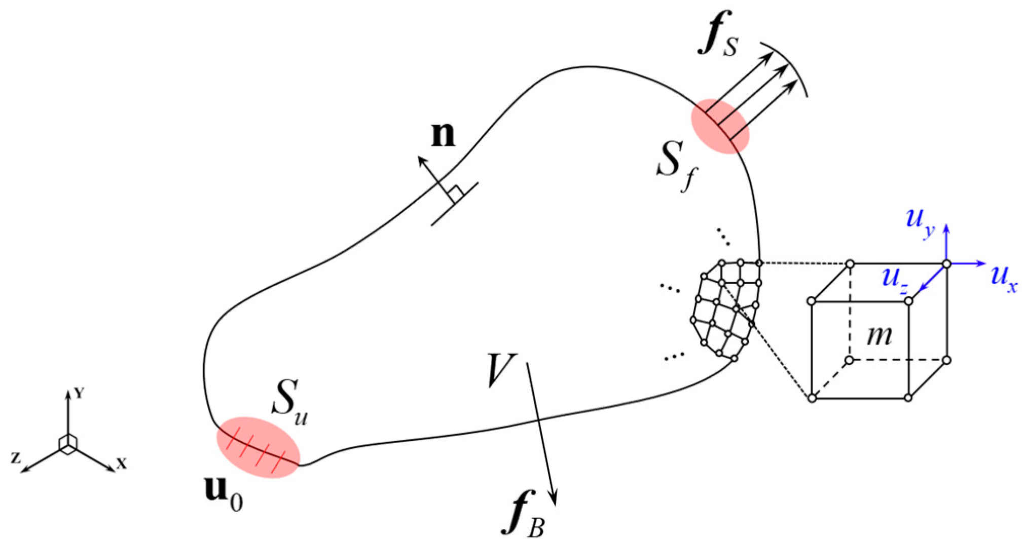
2. FE Formulation for Dynamic Analysis

In this section, we briefly review the FE formulation for dynamic analysis. The detailed formulations and assumptions can be seen in Refs. [17,18]. In FEM, as shown in Figure 1, a continuous body with infinite DOFs is discretized into finite elements with nodes. Thus, the mechanical behavior of the FE model can be expressed with finite DOFs.

For the discretized body, the following equilibrium equations are satisfied

$$\mathsf{\sigma }n=f_S,\nabla \mathsf{\sigma }+f_B=0,u_0=0,$$

(1)

where $\mathsf{\sigma }$ and $f_S$ are the stress matrix and load vector applied to the surface force area $S_f$, and $f_B$ is the body force vector. Here, $\nabla$ and $n$ are a spatial gradient operator and normal vector, respectively. It should be noted that the displacement vector $u_0$ corresponding to the displacement boundary condition area $S_u$ should be a zero vector, because all DOFs are constrained to $S_u$.

For the element $m$, the displacement vector $u^{(m)}$ and the strain vector ${\mathsf{\epsilon }}^{(m)}$ are defined by

$$u^{(m)}=P^{(m)}u,{\mathsf{\epsilon }}^{(m)}=B^{(m)}u,$$

(2)

in which $P^{(m)}$ and $B^{(m)}$ are the displacement interpolation and strain-displacement interpolation matrices, and $u$ is the nodal displacement vector.

The stress vector for the element $m$ is defined by the stress-strain law as

$${\mathsf{\sigma }}^{(m)}=D^{(m)}{\mathsf{\epsilon }}^{(m)},$$

(3)

where $D^{(m)}$ is the stress-strain relation matrix for the element $m$.

Applying the principle of virtual work [4] to Equation (1) and considering the discretization, the following integral equation is obtained

$${\displaystyle {\int }_{V^{(m)}}\delta {\mathsf{\epsilon }}^{(m)}{\mathsf{\sigma }}^{(m)}d{V}^{(m)}}={\displaystyle {\int }_{S_f^{(m)}}\delta u^{(m)}{f}_S^{(m)}d{S}^{(m)}}+{\displaystyle {\int }_{V^{(m)}}\delta u^{(m)}{f}_B^{(m)}d{V}^{(m)}},$$

(4)

in which $\delta {\mathsf{\epsilon }}^{(m)}$ and $\delta u^{(m)}$ are the virtual strain and virtual displacement vectors, respectively, of the element $m$.

Substituting Equations (2) and (3) into Equation (4), and after assembling all elements, we can obtain the static equilibrium equation as follow

$$\begin{gathered} K_g{u}_g=R_g\mathrm{with} \\ {K}_g={\displaystyle \sum _m{\displaystyle {\int }_{V^{(m)}}{(B^{(m)})}^T{D}^{(m)}{B}^{(m)}d{V}^{(m)}}}, \\ {R}_g={\displaystyle \sum _m{\displaystyle {\int }_{V^{(m)}}{P}^{(m)}{f}_B^{(m)}d{V}^{(m)}}}+{\displaystyle \sum _m{\displaystyle {\int }_{S_f^{(m)}}{P}^{(m)}{f}_S^{(m)}d{S}^{(m)}}}, \end{gathered}$$

(5)

where $K_g$ is the global stiffness matrix, and $u_g$ and $R_g$ are the global displacement and load vectors, respectively.

Using d’Alembert’s principle [19], the element inertia force is considered, and $f_B^{(m)}$ in Equation (5) is redefined as

$$f_B^{(m)}=f_B^{(m)}-{\rho }^{(m)}{\ddot{u}}_g-{\mu }^{(m)}{\dot{u}}_g,$$

(6)

in which ${\rho }^{(m)}$ and ${\mu }^{(m)}$ are the mass density and damping property parameter, respectively, of the element $m$, and ${\ddot{u}}_g$ and ${\dot{u}}_g$ are the global acceleration and velocity vectors, respectively.

Substituting Equation (6) into Equation (5), we can obtain the equations of motion for the global system as follows

$$\begin{gathered} M_g{\ddot{u}}_g+C_g{\dot{u}}_g+K_g{u}_g=R_g\mathrm{with} \\ {M}_g={\displaystyle \sum _m{\displaystyle {\int }_{V^{(m)}}{\rho }^{(m)}{(P^{(m)})}^T{P}^{(m)}d{V}^{(m)}}},C_g={\displaystyle \sum _m{\displaystyle {\int }_{V^{(m)}}{\mu }^{(m)}{(P^{(m)})}^T{P}^{(m)}d{V}^{(m)}}}, \end{gathered}$$

(7)

where $M_g$ and $C_g$ denote the global mass and damping matrices, respectively. It should be noted that, in the undamped free vibration system, the global damping matrix $C_g$ and global load vector $R_g$ can be neglected. In general, $R_g$ can be expressed according to the type of external load.

To precisely obtain the damping property parameter $\mu$ in Equation (7), it is required to experiment on a real structure. For convenience, we adopt the following the Rayleigh damping equation [20,21] to assume the global damping matrix $C_g$ as

$$C_g=\alpha M_g+\beta K_g,$$

(8)

in which $\alpha$ and $\beta$ are the proportional damping coefficients. It can be easily seen that the global damping matrix $C_g$ can be calculated with a linear combination of the global mass matrix $M_g$ and stiffness matrix $K_g$.

In Equation (8), the proportional damping parameters $\alpha$ and $\beta$ are determined according to the natural frequencies of the structure and can be calculated using the following equation

$$\left[\begin{array}{cc}1& {\omega }_i^2\\ 1& {\omega }_j^2\end{array}\right]\left[\begin{array}{c}\alpha \\ \beta \end{array}\right]=2\left[\begin{array}{c}{\xi }_i{\omega }_i\\ {\xi }_j{\omega }_j\end{array}\right],$$

(9)

where ${\omega }_i$ and ${\omega }_j$ are the $i^{th}$ and $j^{th}$ natural frequencies of the FE model, respectively, and ${\xi }_i$ and ${\xi }_j$ are the damping ratio of the $i^{th}$ and $j^{th}$ modes, respectively.

When performing dynamic analysis of global structures, numerical calculations must be performed repeatedly using the global matrices ($M_g$, $C_g$, and $K_g$) and the global vectors ($u_g$, ${\dot{u}}_g$, ${\ddot{u}}_g$, and $R_g$). Therefore, it is obvious that a lot of computational cost is consumed when conducting dynamic analysis of large FE models.

3. Construction of Condensed Matrices

In this section, we briefly introduce the construction process of the condensed mass, stiffness, and damping matrices. The detailed derivation procedure is described in Refs. [22,23]. For this, it is essential to partition all DOFs of the FE model into retained and truncated DOFs. Here, retained DOFs are the nodes of interest to be analyzed. Truncated DOFs are the nodes to be condensed out and omitted, because they are not interesting for analysis.

The matrices of the FE model are large and sparse, as shown in Figure 2a. The retained nodes can be selected by engineers via consideration of analysis purposes, and we can assign new node numbers for the selected retained nodes. Then, all remaining nodes are automatically designated as truncated nodes. After this node number assignment, we can obtain the re-ordered and partitioned matrices, as shown in Figure 2b.

After selecting the retained DOFs, the global displacement vector $u_g$ in Equation (5) can be described in the following partitioned form

$$u_g=\left[\begin{array}{c}{u}_t\\ u_r\end{array}\right],$$

(10)

where $u_t$ and $u_r$ are the truncated and retained displacement vectors, respectively.

Similarly, the global mass and stiffness matrices can be expressed in partitioned form, and thus the eigenvalue problem can be written in the following partitioned form

$$\left[\begin{array}{cc}{K}_t& K_c\\ K_c^T& K_r\end{array}\right]\left[\begin{array}{c}{u}_t\\ u_r\end{array}\right]=\lambda \left[\begin{array}{cc}{M}_t& M_c\\ M_c^T& M_r\end{array}\right]\left[\begin{array}{c}{u}_t\\ u_r\end{array}\right],$$

(11)

in which $\lambda$ is an eigenvalue of the global system. The subscript $c$ is a coupled term between the truncated and retained DOFs, denoted by $t$ and $r$.

Expanding the first row in Equation (11), the truncated displacement vector $u_t$ is defined by

$$u_t=-K_t^{-1}{K}_c{u}_r+\lambda K_t^{-1}(M_t{u}_t+M_c{u}_r),$$

(12)

then, assuming a transformation matrix $T$ representing the relationship between $u_t$ and $u_r$, the following equation is obtained

$$u_t=T{u}_r.$$

(13)

Using Equation (13), Equation (12) can be rewritten as

$$u_t=[-K_t^{-1}{K}_c+\lambda K_t^{-1}(M_{t}T+M_c)]u_r,$$

(14)

and we can define the transformation matrix $T$ as

$$T=T_0+T_1\mathrm{with}{T}_0=-K_t^{-1}{K}_c,T_1=\lambda K_t^{-1}(M_{t}T+M_c).$$

(15)

Substituting Equations (14) and (15) into Equation (10), the global displacement vector $u_g$ can be expressed using only the retained displacement vector $u_r$ as

$$u_g=\left[\begin{array}{c}T\\ I_r\end{array}\right]u_r=(T_s+T_d)u_r\mathrm{with}{T}_s=\left[\begin{array}{c}{T}_0\\ I_r\end{array}\right],T_d=\left[\begin{array}{c}{T}_1\\ 0\end{array}\right],$$

(16)

where $T_s$ is the transformation matrix that condenses the stiffness corresponding to the truncated displacement vector $u_t$, and $T_d$ is the transformation matrix that condenses the inertia effect corresponding to $u_t$. Here, $I_r$ is the identity matrix equal to the size of the retained DOFs.

In Equation (16), neglecting $T_d$ because it contains the unknown eigenvalue $\lambda$ in $T_1$, the global displacement vector $u_g$ can be approximated as follows

$$u_g\approx {\widehat{u}}_g=T_s{u}_r,$$

(17)

and substituting Equation (17) into Equation (11), and pre-multiplying both sides by $T_s^T$, the following reduced eigenvalue problem is obtained

$${\widehat{K}}_s{u}_r=\widehat{\lambda }{\widehat{M}}_s{u}_r\mathrm{with}{\widehat{K}}_s=T_s^T{K}_g{T}_s,{\widehat{M}}_s=T_s^T{M}_g{T}_s,$$

(18)

where ${\widehat{M}}_s$ and ${\widehat{K}}_s$ are the mass and stiffness matrices reduced by the stiffness condensation matrix $T_s$, respectively, and $\widehat{\lambda }$ is the eigenvalue defined in the eigenvalue problem considering the stiffness condensation.

In Equation (18), multiplying both sides by ${\widehat{M}}_s^{-1}$, the following equation is obtained

$$\widehat{\lambda }{u}_r={\widehat{M}}_s^{-1}{\widehat{K}}_s{u}_r,$$

(19)

Assuming $\lambda \approx \widehat{\lambda }$ and using the relationship between $\widehat{\lambda }$ and ${\widehat{M}}_s^{-1}{\widehat{K}}_s$ in Equation (19), the transformation matrix $T_1$ in Equation (15) can be rewritten as

$$T_1=K_t^{-1}(M_{t}T+M_c)A\mathrm{with}A={\widehat{M}}_s^{-1}{\widehat{K}}_s,$$

(20)

it should be noted that the transformation matrix $T$ in Equation (13) is implicit because $T$ also exists in $T_1$. Thus, the transformation matrix $T$ can be obtained via iterative calculation.

Using Equations (16), (19) and (20), the iterative transformation matrix $T_{ITER}$ can be expressed as

$$\begin{gathered} T_{ITER}^{(k)}=\left[\begin{array}{c}{T}^{(k)}\\ I_r\end{array}\right],T^{(k)}=T_0+K_t^{-1}(M_t{T}^{(k-1)}+M_c)A^{(k-1)} \\ \mathrm{for}k\ge 2\mathrm{with}{T}^{(1)}=T_0, \end{gathered}$$

(21)

where $T^{(k)}$ is implicit in the formulation, and $k$ is the iteration number.

The term $A^{(k-1)}$ in Equation (21) can be calculated by

$$A^{(k-1)}={({\overline{M}}^{(k-1)})}^{-1}{\overline{K}}^{(k-1)},$$

(22)

$${\overline{M}}^{(k-1)}={(T_{ITER}^{(k-1)})}^T{M}_g{T}_{ITER}^{(k-1)},{\overline{K}}_{}^{(k-1)}={(T_{ITER}^{(k-1)})}^T{K}_g{T}_{ITER}^{(k-1)}\mathrm{for}k\ge 2,$$

(23)

$$T_{ITER}^{(1)}=T_s,{\overline{M}}^{(1)}={\widehat{M}}_s,{\overline{K}}^{(1)}={\widehat{K}}_s.$$

(24)

After the final iteration of $T_{ITER}^{(k)}$ in Equation (21), we can approximate the global displacement vector $u_g$ as

$$u_g\approx {\overline{u}}_g=T_f{u}_r\mathrm{with}{T}_f=T_{ITER}^{(k)},$$

(25)

in which $T_f$ is the final transformation matrix. It should be noted that Equation (25) indicates that the displacement vector of the condensed system $u_r$ can be converted to that of the global system by the transformation matrix $T_f$.

Finally, we can obtain the condensed mass and stiffness matrices as follows

$$\overline{M}=T_f^T{M}_g{T}_f,\overline{K}=T_f^T{K}_g{T}_f.$$

(26)

It should be noted that, although $\overline{M}$ and $\overline{K}$ are expressed with the retained DOFs only, they contain the stiffness and inertia effects corresponding to the truncated DOFs.

As mentioned in Equation (8), the global damping matrix $C_g$ is calculated with a linear combination of the global mass and stiffness matrices. Therefore, in the same manner, we can obtain the condensed damping matrix as follows

$$\overline{C}=\alpha \overline{M}+\beta \overline{K}.$$

(27)

4. Structural Dynamic Formulations Using Condensed Matrices

In this section, using the condensed matrices $\overline{M}$, $\overline{C}$, and $\overline{K}$, obtained in the previous section, we derive the formulations for the modal, frequency response, and transient analyses.

4.1. Modal Analysis

Modal analysis, known as a free vibration analysis, is frequently used to identify natural frequencies and corresponding mode shapes of structures. The equations of motion of the global system for undamped free vibration are written as follows

$$M_g{\ddot{u}}_g+K_g{u}_g=0.$$

(28)

By differentiating ${\overline{u}}_g$ in Equation (25) twice with respect to time $t$, the approximated acceleration vector is defined as

$${\ddot{\overline{u}}}_g=T_f{\ddot{u}}_r.$$

(29)

Substituting Equations (25) and (29) into Equation (28), the following equation is obtained

$$M_g{T}_f{\ddot{u}}_r+K_g{T}_f{u}_r=0,$$

(30)

multiplying by $T_f^T$, we can obtain the condensed formulation for the free vibration as follows

$$\overline{M}{\ddot{u}}_r+\overline{K}{u}_r=0,$$

(31)

it should be noted that $\overline{M}$ and $\overline{K}$ are the condensed mass and stiffness matrices, already calculated from Equation (26).

For the retained displacement vector $u_r$ in Equation (31), the following assumptions for the displacement and acceleration vectors can be derived

$$u_r={\mathsf{\phi }}_r\sin (\omega t+\theta ),{\ddot{u}}_r=-{\omega }^2{\mathsf{\phi }}_r\sin (\omega t+\theta ),$$

(32)

where ${\mathsf{\phi }}_r$ is the amplitude vector corresponding to $u_r$. Here, $\omega$ and $\theta$ are the natural frequency and phase angle corresponding to $u_r$, respectively.

Substituting Equation (32) into Equation (31), and neglecting $\sin (\omega t+\theta )$, we can obtain the condensed formulation for modal analysis as follows

$$\overline{K}{\mathsf{\phi }}_r={\omega }^2\overline{M}{\mathsf{\phi }}_r,$$

(33)

in which the amplitude vector ${\mathsf{\phi }}_r$ is identical to the eigenvector of the condensed system and is also regarded as the mode shape of the condensed system. ${\omega }^2$ is identical with the eigenvalue of the condensed system.

However, the mode shape ${\mathsf{\phi }}_r$ in Equation (33) contains only information corresponding to the retained DOFs. Therefore, to obtain the mode shape for the global structure, the following back transformation process is required. Using the relation ${\overline{u}}_g=T_f{u}_r$ in Equation (25), we can approximate the global mode shape as

$${\overline{\mathsf{\phi }}}_g=T_f{\mathsf{\phi }}_r.$$

(34)

Thus, we can conclude that, by solving the condensed formulation for modal analysis in Equation (33), which is computed with very small size matrices, and using the back transformation process in Equation (34), we can very effectively approximate the natural frequency and its corresponding mode shape for the global structure. The computational efficiency and solution accuracy will be precisely demonstrated in Section 5.

4.2. Frequency Response Analysis

For frequency response analysis with damping and excitation load, we can consider the following equations of motion for the global system:

$$M_g{\ddot{u}}_g+C_g{\dot{u}}_g+K_g{u}_g=R_g.$$

(35)

By differentiating ${\overline{u}}_g$ in Equation (25) with respect to time $t$, the approximated velocity vector is defined as

$${\dot{\overline{u}}}_g=T_f{\dot{u}}_r.$$

(36)

Using ${\ddot{\overline{u}}}_g=T_f{\ddot{u}}_r$ in Equation (29) and ${\dot{\overline{u}}}_g=T_f{\dot{u}}_r$ in Equation (36), and multiplying by $T_f^T$, we can obtain the condensed dynamic formulation considering the damping effect and the excitation load as

$$\overline{M}{\ddot{u}}_r+\overline{C}{\dot{u}}_r+\overline{K}{u}_r=\overline{R}\mathrm{with}\overline{R}=T_f^T{R}_g,$$

(37)

where $\overline{R}$ is the condensed load vector.

In Equation (37), the condensed load vector $\overline{R}$ can be assumed to be the harmonic forcing function represented in complex form, and Equation (37) can be rewritten as

$$\overline{M}{\ddot{u}}_r+\overline{C}{\dot{u}}_r+\overline{K}{u}_r=\overline{R}{e}^{i{\omega }_{0}t},$$

(38)

in which ${\omega }_0$ denotes the excitation frequency.

The particular solution for the retained displacement vector $u_r$ can be written as

$$u_r(t)=X_r{e}^{i{\omega }_{0}t},$$

(39)

and the velocity and acceleration vectors can be written as

$${\dot{u}}_r(t)=i{\omega }_0{X}_r{e}^{i{\omega }_{0}t},{\ddot{u}}_r(t)=-{\omega }_0^2{X}_r{e}^{i{\omega }_{0}t},$$

(40)

where $X_r$ is the response amplitude vector for the retained displacement vector $u_r$.

Substituting Equations (39) and (40) into Equation (38), the condensed response amplitude vector $X_r$ can be expressed with the function of the excitation frequency ${\omega }_0$ as

$$X_r({\omega }_0)=\overline{H}\overline{R}\mathrm{with}\overline{H}={(-{\omega }_0^2\overline{M}+i{\omega }_0\overline{C}+\overline{K})}^{-1},$$

(41)

in which $\overline{H}$ represents the complex frequency response function (FRF) matrix of the condensed system. It should be noted that, to calculate $X_r({\omega }_0)$, an iterative calculation must be performed considering the excitation frequency range of interest and the excitation frequency ${\omega }_0$, defined incrementally.

The condensed response amplitude vector $X_r({\omega }_0)$ in Equation (41) can be divided into a real term and an imaginary term and the magnitude vector $\left|X_r({\omega }_0)\right|$ is defined as

$$\left|X_r({\omega }_0)\right|=\sqrt{{\{\mathrm{Re}(X_r)\}}^2+{\{\mathrm{Im}(X_r)\}}^2}.$$

(42)

Using the relation between the condensed and global systems that is defined by the transformation matrix $T_f$, we can obtain the following equation

$$\left|{\overline{X}}_g({\omega }_0)\right|=T_f\left|X_r({\omega }_0)\right|,$$

(43)

where $\left|{\overline{X}}_g({\omega }_0)\right|$ is the approximated response amplitude vector for the global structure.

4.3. Transient Analysis

To analyze the transient responses of structures, the Newmark method [24] has been widely used in structural dynamics. Based on this method, condensed transient analysis formulation is derived as follows.

The equation of motion for the condensed system at time $t+\Delta t$ can be expressed as

$$\overline{M}{\ddot{u}}_r^{t+\Delta t}+\overline{C}{\dot{u}}_r^{t+\Delta t}+\overline{K}{u}_r^{t+\Delta t}={\overline{R}}^{t+\Delta t},$$

(44)

where ${\ddot{u}}_r^{t+\Delta t}$, ${\dot{u}}_r^{t+\Delta t}$, and $u_r^{t+\Delta t}$ are the condensed acceleration, velocity, and displacement vectors at time $t+\Delta t$, respectively, and ${\overline{R}}^{t+\Delta t}$ is the condensed load vector at time $t+\Delta t$.

However, the condensed acceleration, velocity, and displacement vectors at time $t+\Delta t$ (${\ddot{u}}_r^{t+\Delta t}$, ${\dot{u}}_r^{t+\Delta t}$, and $u_r^{t+\Delta t}$) are unknown values. To handle these unknowns, we can assume that the condensed acceleration vector ${\ddot{u}}_r^{t+\Delta t}$ [25] between two instants of time, as shown in Figure 3. On the other hand, according to the initial condition, the condensed acceleration, velocity, and displacement vectors at time $t$ (${\ddot{u}}_r^t$, ${\dot{u}}_r^t$, and $u_r^t$) are known values.

Using the constant-average acceleration, we can define the condensed acceleration vector at time $t+\tau$ as follows

$${\ddot{u}}_r(t+\tau )=0.5({\ddot{u}}_r^{t+\Delta t}+{\ddot{u}}_r^t)\mathrm{with}t\le t+\tau \le t+\Delta t,$$

(45)

where $t+\tau$ is the time between $t$ and $t+\Delta t$.

By integrating Equation (45) with respect to time $t$, we can assume the condensed velocity and displacement vectors as follows

$${\dot{u}}_r(t+\tau )={\dot{u}}_r^t+0.5({\ddot{u}}_r^{t+\Delta t}+{\ddot{u}}_r^t)\tau ,$$

(46)

$$u_r(t+\tau )=u_r^t+\tau u_r^t+0.25({\ddot{u}}_r^{t+\Delta t}+{\ddot{u}}_r^t){\tau }^2.$$

(47)

Using Equations (46) and (47), we can obtain the condensed velocity and displacement vectors in the general form when $\tau =\Delta t$, as follows

$${\dot{u}}_r^{t+\Delta t}={\dot{u}}_r^t+\Delta t[(1-\delta ){\ddot{u}}_r^t+\delta {\ddot{u}}_r^{t+\Delta t}],$$

(48)

$$u_r^{t+\Delta t}=u_r^t+\Delta t{\dot{u}}_r^t+\Delta t^2[(0.5-\gamma ){\ddot{u}}_r^t+\gamma {\ddot{u}}_r^{t+\Delta t}],$$

(49)

in which $\delta$ and $\gamma$ are the parameters to be determined to obtain the integration accuracy and stability [26]. It should be noted that, because the Newmark method is unconditionally stable when using the constant-average acceleration with $\delta =0.5$ and $\gamma =0.25$, we use these parameters in this study.

Rearranging Equation (49) for ${\ddot{u}}_r^{t+\Delta t}$, the condensed acceleration vector at time $t+\Delta t$ is defined as

$${\ddot{u}}_r^{t+\Delta t}=\frac{1}{\gamma \Delta t^2}(u_r^{t+\Delta t}-u_r^t)-\frac{1}{\gamma \Delta t}{\dot{u}}_r^t-\left(\frac{1}{2\gamma }-1\right){\ddot{u}}_r^t.$$

(50)

Substituting Equations (48) and (50) into Equation (44) and rearranging for $u_r^{t+\Delta t}$, we can obtain the equation for the condensed displacement vector $u_r^{t+\Delta t}$ as follows

$$\begin{gathered} u_r^{t+\Delta t}={\tilde{K}}^{-1}{\tilde{R}}^{t+\Delta t}\mathrm{with}\tilde{K}=a_0\overline{M}+a_1\overline{C}+\overline{K}, \\ {\tilde{R}}^{t+\Delta t}=[{\overline{R}}^{t+\Delta t}+\overline{M}(a_0{u}_r^t+a_2{\dot{u}}_r^t+a_3{\ddot{u}}_r^t)+\overline{C}(a_1{u}_r^t+a_4{\dot{u}}_r^t+a_5{\ddot{u}}_r^t)] \end{gathered}$$

(51)

where $a_0$, $a_1$, $a_2$, $a_3$, $a_4$, and $a_5$ are the integration constants. We can obtain the condensed displacement vector at time $t+\Delta t$ ($u_r^{t+\Delta t}$) at each time step by using Equation (51). Then, using Equations (48) and (50), the condensed velocity and acceleration vectors, ${\dot{u}}_r^{t+\Delta t}$ and ${\ddot{u}}_r^{t+\Delta t}$, are calculated, respectively.

In Equation (51), the integration constants, $a_0$ to $a_5$, are defined as

$$\begin{gathered} a_0=\frac{1}{\gamma \Delta t^2},a_1=\frac{\delta }{\gamma \Delta t},a_2=\frac{1}{\gamma \Delta t}, \\ {a}_3=\frac{1-2\gamma }{2\gamma },a_4=\frac{\delta -\gamma }{\gamma },a_5=\frac{\Delta t}{2}\left(\frac{\delta }{\gamma }-2\right). \end{gathered}$$

(52)

Using the relation ${\overline{u}}_g=T_f{u}_r$ in Equation (25), we can obtain the approximated global displacement, velocity, and acceleration vectors at each time step, as follows

$${\overline{u}}_g^{t+\Delta t}=T_f{u}_r^{t+\Delta t},{\dot{\overline{u}}}_g^{t+\Delta t}=T_f{\dot{u}}_r^{t+\Delta t},{\ddot{\overline{u}}}_g^{t+\Delta t}=T_f{\ddot{u}}_r^{t+\Delta t}.$$

(53)

Finally, unlike structural dynamic analysis using global matrices ($M_g$, $C_g$, and $K_g$), we use condensed matrices ($\overline{M}$, $\overline{C}$, and $\overline{K}$). The resulting computational advantage of using these condensed matrices will be discussed and analyzed specifically in the following section.

5. Structural Dynamic Analysis for a Stiffened Plate

In this section, using the condensed formulations presented in the previous, we conducted modal, frequency response, and transient analyses for a stiffened plate, a primal structural unit for ship and offshore structures.

As shown in Figure 4, we used a cross-stiffened plate representing a typical bottom component of ship and offshore structures. The dimensions of the stiffened plate were length $\mathrm{L}=7620\mathrm{mm}$, breadth $\mathrm{B}=3480\mathrm{mm}$, transverse frame spacing $\mathrm{l}=1524\mathrm{mm}$, and longitudinal spacing $\mathrm{b}=304\mathrm{mm}$. The thickness of the plate was $7\mathrm{mm}$ and clamped boundary conditions were imposed at both ends. The stiffened plate consisted of 9 longitudinal and 4 transverse frames. The dimensions of the frames are shown in Figure 4.

The stiffened plate FE model was expressed using Abaqus 2022, and it contains 6393 4-node quadrilateral (S4R) shell elements [27], and 38,712 DOFs. The material was a mild steel (Young’s modulus $\mathrm{E}=206\mathrm{GPa}$, Poisson’s ratio $\mathsf{\upsilon }=0.3$, density $\mathsf{\rho }=7850{\mathrm{kg}/\mathrm{m}}^3$, and the damping ratio $\mathsf{\xi }=0.01$). All the computer codes were implemented in MATLAB R2021a, and computation was performed on a personal computer (Intel i7-8700 CPU and 32GB RAM).

In the modal analysis, to verify the solution reliability of the condensed system, we precisely compared the natural frequencies and mode shapes calculated from the global and condensed systems. In the frequency response analysis, the approximated response amplitude results according to the excitation frequency range of interest were calculated and compared. In the transient analysis, the approximated displacement, velocity, and acceleration results with time history were investigated. Additionally, the computation times for these analyses were measured and analyzed to closely validate the computational efficiency of the condensed system. The procedures to calculate the condensed matrices ($\overline{M}$, $\overline{K}$, and $\overline{C}$) are described in Figure 5. To extract the global mass and stiffness matrices ($M_g$ and $K_g$), Abaqus ‘MATRIX GENERATE’ function was used. It should be noted that the accuracy of the condensed matrices is affected by the iteration number $k$, determined by the engineer in consideration of the desired level of solution accuracy. In this study, we used the iteration number $k=10$.

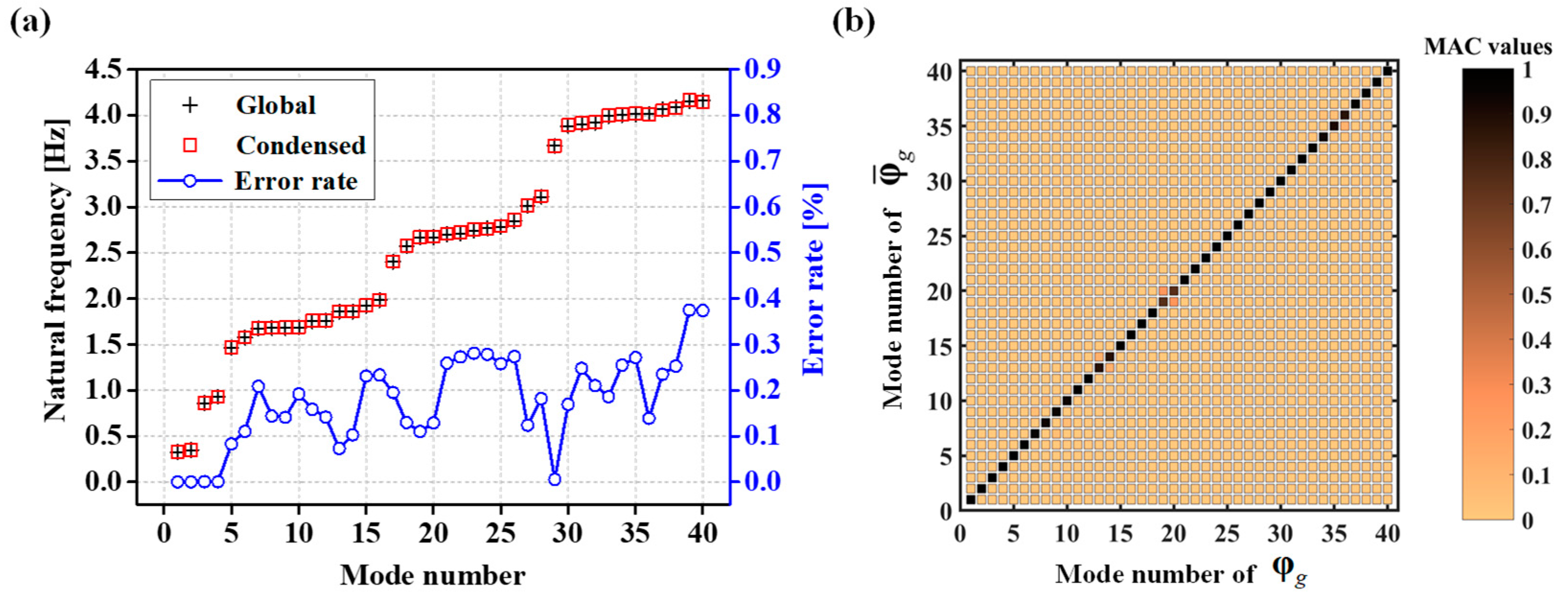
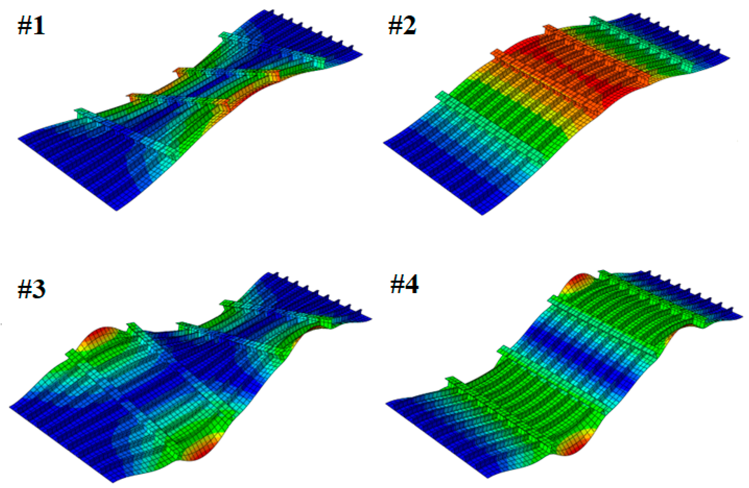
5.1. Modal Analysis Results

In the modal analysis, we condensed the global stiffened FE model with 50 retained nodes. To select these retained nodes, we adapted the node selection method [28] using the ratio of the diagonal terms of the mass and stiffness matrices. Here, the nodes with high ratio values were the dominant nodes used to express the dynamic behavior of the system. For the considered stiffened FE model, we selected the top 50 nodes with high ratio values; condensed matrices with 300 DOFs were obtained.

Then, solving the condensed eigenvalue problem $\overline{K}{\mathsf{\phi }}_r={\omega }^2\overline{M}{\mathsf{\phi }}_r$ described in Equation (33) with $\overline{M}$ and $\overline{K}$, we calculated 40 natural frequencies and mode shapes of the condensed system ${\mathsf{\phi }}_r$. Using the relation ${\overline{\mathsf{\phi }}}_g=T_f{\mathsf{\phi }}_r$ described in Equation (34), we were able to calculate 40 approximated global mode shapes ${\overline{\mathsf{\phi }}}_g$.

To verify the reliability of the natural frequencies calculated from the condensed system, the error rate was calculated as follows

$$e_j=\frac{\left|{\overline{\omega }}_j-{\omega }_j\right|}{{\omega }_j}\times 100[\%]\mathrm{with}j=1,2,3,\dots ,$$

(54)

where $e_j$ is the error rate for the $j^{th}$ natural frequency, and ${\omega }_j$ and ${\overline{\omega }}_j$ are the $j^{th}$ natural frequencies of the global and condensed systems, respectively.

The mode shapes were compared with the following modal assurance criterion (MAC) [29] as

$$MAC=\frac{{\left|{({\mathsf{\phi }}_g)}_v^T\cdot {({\overline{\mathsf{\phi }}}_g)}_w\right|}^2}{\{{({\mathsf{\phi }}_g)}_v^T\cdot {({\mathsf{\phi }}_g)}_w\}\{{({\overline{\mathsf{\phi }}}_g)}_v^T\cdot {({\overline{\mathsf{\phi }}}_g)}_w\}}\mathrm{with}v,w=1,2,\dots ,j,$$

(55)

in which ${\mathsf{\phi }}_g$ and ${\overline{\mathsf{\phi }}}_g$ are the mode shapes calculated from the global and condensed systems, respectively. It should be noted that, to check the consistency of the two mode shapes, the MAC values appear in matrix form and are expressed as values between 0 to 1. The closer the values are to 1, the more consistent the mode shapes are considered to be.

Figure 6 shows the natural frequencies, error rates of the natural frequencies, and MAC values corresponding to the 1st–40th modes. The exact natural frequencies for the 1st and the 40th modes were 0.326 Hz and 4.162 Hz, and the corresponding approximated natural frequencies were 0.326 Hz and 4.147 Hz. As shown in Figure 6a, the natural frequencies calculated from the condensed system were nearly identical to those of the global system. As shown in Figure 6b, all diagonal terms of MAC values were close to 1, and it could be concluded that the approximated global mode shapes ${\overline{\mathsf{\phi }}}_g$ determined using the proposed formulation were highly consistent with the global mode shapes ${\mathsf{\phi }}_g$ of the global system.

Figure 7 shows the 1st–4th mode shapes of the stiffened FE model.

Table 1. Natural frequencies, error rates, and MAC values for 10 modes with the largest error.

Mode Number	Natural Frequency ω [Hz]		Error Rate ej [%]	MAC Values
	Global	Condensed
39	4.151	4.166	0.361	0.998
40	4.162	4.147	0.360	0.995
23	2.744	2.752	0.292	0.999
26	2.848	2.856	0.281	1.000
35	4.010	4.021	0.274	0.989
21	2.700	2.707	0.259	0.990
22	2.713	2.720	0.258	0.989
24	2.768	2.761	0.253	0.994
25	2.785	2.792	0.251	0.994
34	4.001	4.011	0.250	0.957

lists the natural frequencies, MAC values, and error rates for the 10 modes with the largest error. The maximum error rate was only 0.361% at the 39th mode.

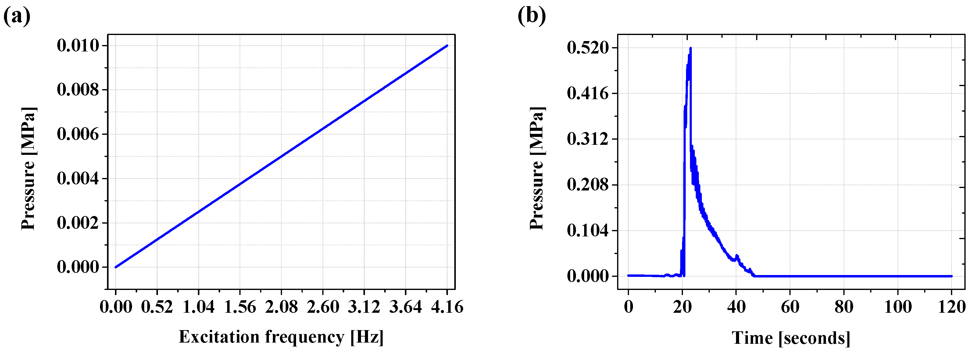
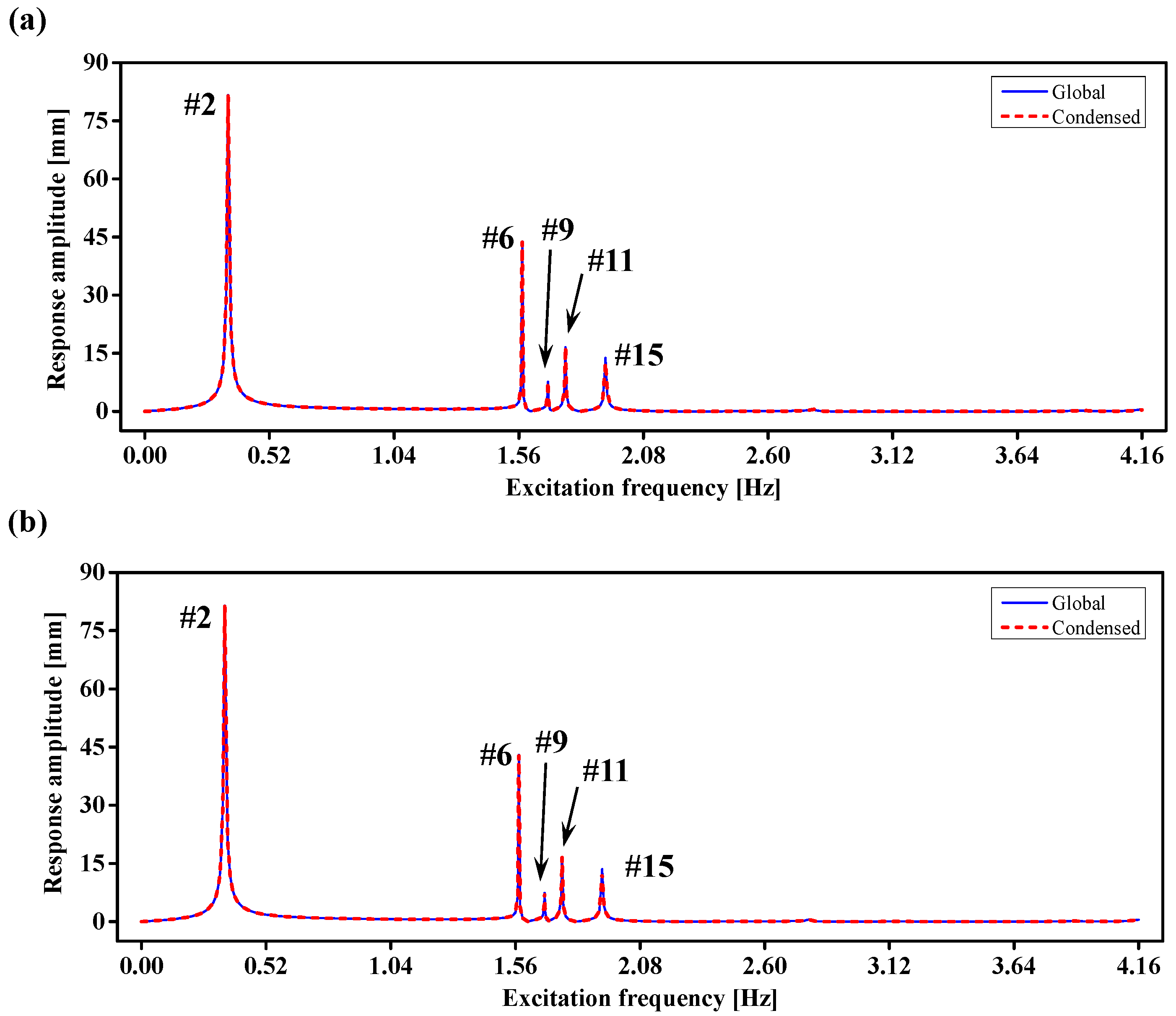
5.2. Frequency Response and Transient Analysis Results

In this section, we demonstrate the solution accuracy of the proposed formulation for the frequency response and transient analyses.

Table 2. Analysis conditions for frequency response and transient analyses.

Analysis	Conditions
Frequency response	Analysis ${\omega }_0$ range	0~4.16 Hz
	$\Delta {\omega }_0$	0.01 Hz
Transient	Analysis $t$ range	0~120 s
	$\Delta t$	0.05 s

shows the analysis conditions. The frequency range and increments for the frequency response analysis and the time range and increment for the transient analysis are listed.

The load profiles for the analyses are shown in Figure 8. In the frequency response analysis, to investigate the resonance behavior within the 1st–40th modes, a linearly increasing pressure was applied within the excitation frequency range of interest from 0 Hz to 4.16 Hz considering the modal analysis results shown in Figure 6a. In the transient response analysis, the time-history load obtained from computational fluid dynamics (CFD) analysis was applied from 0 to 120 s.

As shown in Figure 9, pressure was applied at the bottom of the stiffened plate, and a clamped boundary condition was imposed at both ends. The 27 nodes at the middle of the plate, where large displacements were expected, were selected as the retained nodes. Thus, the total number of retained nodes becomes 77 in the consideration of the 50 retained nodes defined in the previous modal analysis. Therefore, condensed matrices with sizes of $462\times 462$ can be obtained and these matrices were used for the frequency response and transient analyses. Compared to the size of global matrix in the global system ($38,712\times 38,712$), the condensed system contains only 1.193% of the total DOFs.

To calculate the proportional damping coefficients $\alpha$ and $\beta$ used in Equation (8), we used the 1st and 2nd natural frequencies already calculated in the previous modal analysis. Using Equation (9), we could calculate these coefficients as $\alpha =2.47\times {10}^{-17}$ and $\beta =0.02$. Using these, we calculated the damping matrix and use it for the frequency response and transient analyses.

To verify the solution of the frequency response analysis, we compared the response amplitude vectors calculated from the global and condensed models. By solving Equation (41), the condensed response amplitude vector $X_r({\omega }_0)$ was obtained and, using the relation $\left|{\overline{X}}_g({\omega }_0)\right|=T_f\left|X_r({\omega }_0)\right|$ in Equation (43), we obtained the approximated response amplitude $\left|{\overline{X}}_g({\omega }_0)\right|$. The global response amplitude vector $\left|X_g({\omega }_0)\right|$, which is an exact solution, was calculated by solving the following equation

$$X_g({\omega }_0)=H_g{R}_g\mathrm{with}{H}_g={(-{\omega }_0^2{M}_g+i{\omega }_0{C}_g+K_g)}^{-1}.$$

(56)

It should be noted that, since the increment of the excitation frequency is 0.01 Hz within the frequency response analysis range of interest, 417 iterations of computation were performed at the global matrix computing level to calculate the responses. Responses were analyzed at the three nodes of interest on the stiffened plate, indicated in Figure 9.

Figure 10 presents the results of the frequency response analysis for the nodes of interest (#1 and #2 nodes). For the given load profile and the nodes, resonances occurred at the 2nd, 6th, 9th, 11th, and 15th modes.

Table 3. Response amplitude at resonance and errors between global and condensed models.

Node Number	Mode Number	Resonance Response Amplitude [mm]		Error [%]
		Global	Condensed
#1	2	81.570	81.244	0.400
	6	43.848	43.575	0.623
	9	7.646	7.494	1.988
	11	16.572	16.241	1.997
	15	13.779	13.333	3.237
#2	2	81.499	81.265	0.287
	6	43.012	42.718	0.684
	9	7.432	7.311	1.628
	11	16.639	16.267	2.236
	15	13.546	13.029	3.817

lists the values of the resonance response amplitude and the errors between the global and condensed models. In all two nodes of interest, the largest errors occurred at the 15th mode; error values are 3.237% and 3.817%, respectively. In the frequency range of interest, except for the resonance frequencies, the error was less than 0.3%, showing excellent accuracy.

In the transient analysis, we investigated the global displacement, velocity, and acceleration vectors calculated from the global and condensed models. Using Equations (51) and (53), the approximated global displacement, velocity, and acceleration vectors, ${\overline{u}}_g^{t+\Delta t}$, ${\dot{\overline{u}}}_g^{t+\Delta t}$, and ${\ddot{\overline{u}}}_g^{t+\Delta t}$, were obtained. The exact displacement solution corresponding to the global model $u_g^{t+\Delta t}$ was computed by solving the following equation

$$\begin{gathered} u_g^{t+\Delta t}={\tilde{K}}_g^{-1}{\tilde{R}}_g^{t+\Delta t}\mathrm{with}{\tilde{K}}_g=a_0{M}_g+a_1{C}_g+K_g, \\ {\tilde{R}}_g^{t+\Delta t}=[R_g^{t+\Delta t}+M_g(a_0{u}_g^t+a_2{\dot{u}}_g^t+a_3{\ddot{u}}_g^t)+C_g(a_1{u}_g^t+a_4{\dot{u}}_g^t+a_5{\ddot{u}}_g^t)]. \end{gathered}$$

(57)

Then, the exact velocity and acceleration solutions, ${\dot{u}}_g^{t+\Delta t}$ and ${\ddot{u}}_g^{t+\Delta t}$, were calculated by time integration for $u_g^{t+\Delta t}$.

As shown in Figure 8, the load varies for 120 s, and the time-history load, 0.519 MPa, was applied at 23.1 s. Thereafter, the magnitude of the load gradually decreases, and 0 MPa was applied after 46.7 s. To sufficiently observe the response and the damping effect due to the time-history load, the time increment was as set to 0.05 s. Therefore, 2401 iterations of computation were performed at the global matrix computing level to calculate the time varying responses. The transient responses were analyzed for the y-direction, which was the same direction as the time-history load, for the three nodes of interest.

Figure 11 and Figure 12 show the displacement, velocity, and acceleration results, which are the results of the transient analysis for all nodes of interest. From the displacement results, it can be seen that the largest displacement occurs at 23.1 s, when the time-history load was applied. After that, all responses (displacement, velocity, and acceleration) converged to zero by the damping effect. Similar to the displacement results, the velocity and acceleration response results also converge to zero. The maximum displacement, velocity, and acceleration results obtained from the global and condensed models, and their errors, are listed in

Table 4. Maximum displacement, velocity, and acceleration results obtained from global and condensed models, and their errors.

Node Number	Maximum Result	Global	Condensed	Error [%]
#1	Displacement [mm]	10.652	10.656	0.038
	Velocity [mm/s]	10.351	10.354	0.029
	Acceleration [mm/s2]	40.284	40.272	0.030
#2	Displacement [mm]	14.139	14.134	0.035
	Velocity [mm/s]	13.921	13.914	0.050
	Acceleration [mm/s2]	48.849	48.829	0.041

. At the #1 node, the exact solutions for displacement, velocity, and acceleration were 10.652 mm, 10.351 mm/s, and 40.284 mm/s², respectively, and at the #2 node, 14.139 mm, 13.921 mm/s and 48.849 mm/s². The corresponding approximated solutions were 10.656 mm, 10.354 mm/s, and 40.272 mm/s² for the #1 node, and 14.134 mm, 13.914 mm/s and 48.829 mm/s² for the #2 node. The maximum errors at the #1 node were 0.038%, 0.029% and 0.030% for the approximated global displacement, velocity, and acceleration results; at the #2 node, errors were 0.035%, 0.050% and 0.041%, respectively. From these results, it was confirmed that the condensed model can provide very accurate solutions in transient analysis.

5.3. Computational Efficiency Analysis

The computational efficiency of the proposed method was closely verified through the structural dynamic analysis of the stiffened plate. Figure 13 and

Table 5. Computation time for each item for structural dynamic analysis of stiffened plate.

Methods	Items	Computation Time
		[Seconds]	[%]
Global	Modal analysis	7.441	0.417
	Frequency response analysis	731.351	41.014
	Transient analysis	1044.403	58.569
	Total	1783.195	100.000
Condensed	Calculating of the condensed matrices	400.679	22.470
	Modal analysis	0.177	0.010
	Frequency response analysis	10.078	0.565
	Transient analysis	1.599	0.090
	Total	412.533	23.134

show the computation time for each item for structural dynamic analysis of the stiffened plate. When performing the analysis, the total computation time required was 1783.195 s when using the global matrices and 412.533 s when using the condensed matrices.

This means that the proposed method can provide highly accurate solutions using only 23.134% of the total computation time spent handling the global matrices. More attractively, once the condensed matrices were calculated, in case of the proposed method, only 0.665% of the total computation time was required for the structural dynamics analysis. The reason for this is that, in the analysis using the global matrices, iterative calculations were performed on relatively huge matrices. However, in the proposed method, very tiny, condensed matrices were used for the iterations.

6. Conclusions

In this study, we proposed effective formulations for modal, frequency response, and transient analyses using the condensed mass, stiffness, and damping matrices. To construct the condensed mass and stiffness matrices, a transformation matrix was calculated to reflect the stiffness and inertial effects of neglected nodes into the nodes of interest by applying the IIRS method. Then, using the Rayleigh damping equation, the condensed damping matrix was calculated. Using these three condensed matrices, we derived the formulations for the modal, frequency response, and transient analyses, and applied them to the stiffened plate FE model. The accuracy and computational efficiency were investigated, and the following conclusions were drawn from the results.

• Using the proposed formulation for modal analysis, the natural frequencies and mode shapes were calculated for 40 modes, and the maximum errors for these were 0.361%, confirming that solutions with very high accuracy were derived.
• In the frequency response analysis, all errors resulting from the proposed formulation were less than 0.3% in all frequency ranges except for the resonance frequencies, showing excellent accuracy. For the resonance frequencies, the maximum error was 3.817%.
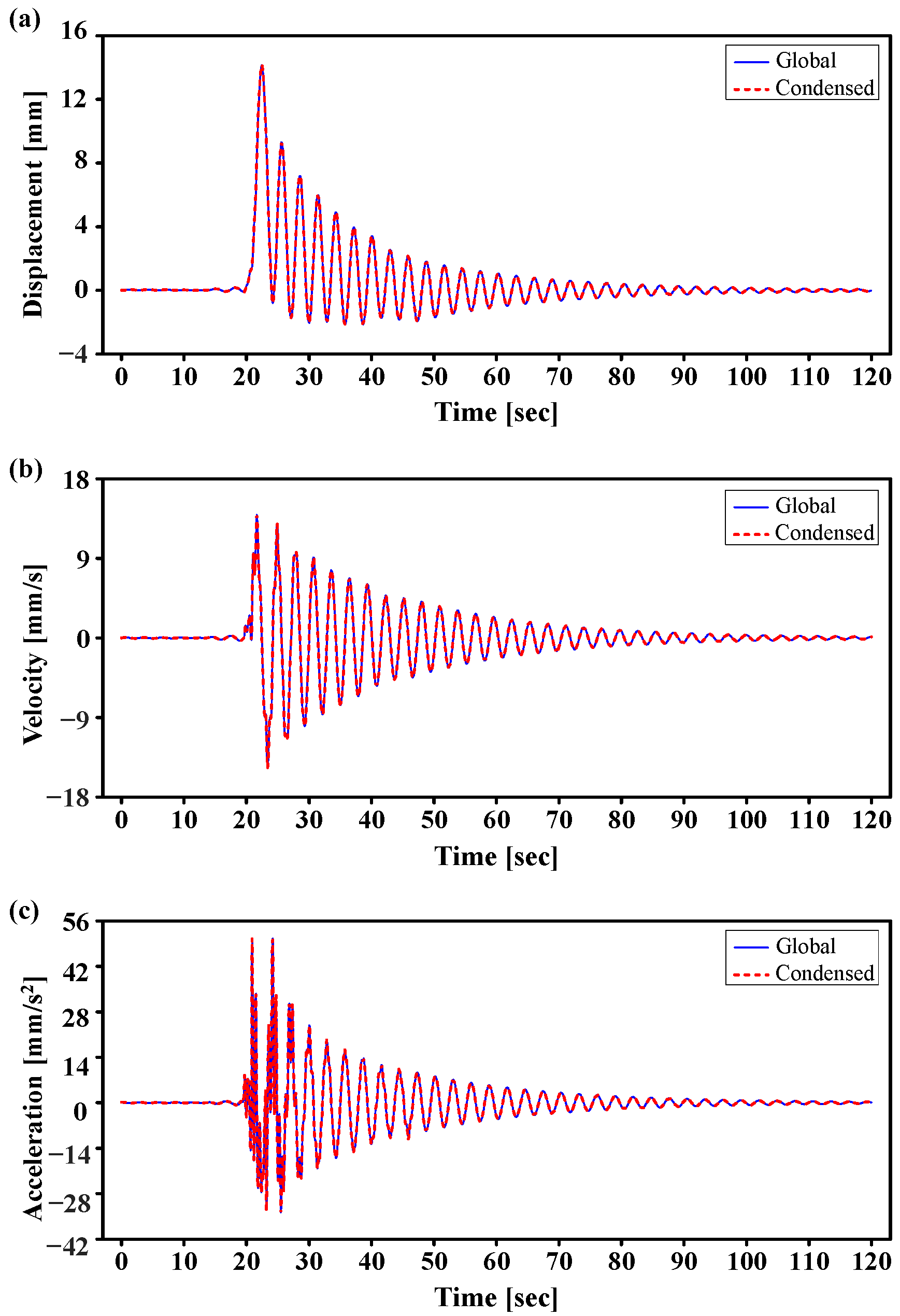
• In the transient analysis, all errors were less than 0.070% for the displacement, velocity, and acceleration results obtained from the condensed model, also showing excellent accuracy.
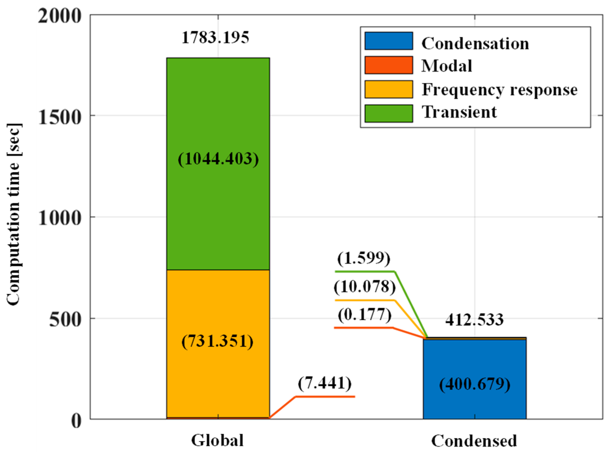
• The proposed formulations provided highly accurate solutions for the structural dynamic analysis, with excellent computational efficiency. Once the condensed matrices were calculated, the computation time for the structural dynamics analysis was only 0.665% of the total computation time, a very attractive aspect of the proposed method.
• In future work, it will be valuable to apply the condensed matrices to other practical engineering and design problems, such as fatigue, quasi-static, local impact, and transient conduction-radiation analyses [30].

References

1. Kirk, C.L. Natural frequencies of stiffened rectangular plates. J. Sound Vib. 1970, 13, 375–388. [Google Scholar] [CrossRef]
2. Gong, S.W.; Lam, K.Y. Transient response of stiffened composite plates subjected to low velocity impact. Compos. Pt. B-Eng. 1998, 30, 473–484. Available online: https://www.sciencedirect.com/science/article/abs/pii/S1359836899000025?via%3Dihub (accessed on 1 October 2022). [CrossRef]
3. Bathe, K.J. Finite Element Procedure; Prentice Hall: Hoboken, NJ, USA, 2006. [Google Scholar]
4. Feriani, A.; Perotti, F.; Simoncini, V. Iterative system solvers for the frequency analysis of linear mechanical systems. Comput. Meth. Appl. Mech. Eng. 2000, 190, 1719–1739. [Google Scholar] [CrossRef]
5. Kim, H.; Melhem, H. Damage detection of structures by wavelet analysis. Eng. Struct. 2004, 26, 347–362. [Google Scholar] [CrossRef]
6. Ramos, L.F.; Aguilar, R.; Lourenco, P.B.; Moreira, S. Dynamic structural health monitoring of Saint Torcato church. Mech. Syst. Signal Proc. 2013, 35, 1–15. [Google Scholar] [CrossRef]
7. Yue, N.; Khodael, Z.S.; Aliabadi, M.H. Damage detection in large composite stiffened panels based on a novel SHM building block philosophy. Smart Mater. Struct. 2021, 30, 045004. [Google Scholar] [CrossRef]
8. Guyan, R.J. Reduction of stiffness and mass matrices. AIAA 1965, 3, 380. [Google Scholar] [CrossRef]
9. O’Callahan, J. A procedure for an improved reduced system (IRS) model. In Proceedings of the 7th International Modal Analysis Conference, Las Vegas, NV, USA, 30 January–1 February 1989; pp. 17–21. [Google Scholar]
10. Friswell, M.I.; Garvey, S.D.; Penny, J.E.T. Model reduction using dynamic and iterated IRS techniques. J. Sound Vib. 1995, 186, 311–323. [Google Scholar] [CrossRef]
11. Friswell, M.I.; Garvey, S.D.; Penny, J.E.T. The convergence of the iterated IRS method. J. Sound Vib. 1998, 211, 123–132. [Google Scholar] [CrossRef]
12. Qu, Z.Q.; Fu, Z.F. An iterative method for dynamic condensation of structural matrices. Mech. Syst. Signal Proc. 2000, 14, 667–678. [Google Scholar] [CrossRef]
13. Li, W.M.; Hong, J.Z. New iterative method for model updating based on model reduction. Mech. Syst. Signal Proc. 2011, 25, 180–192. [Google Scholar] [CrossRef]
14. Luo, K.; Liu, C.; Tian, Q.; Hu, H. An efficient model reduction method for buckling analyses of thin shells based on IGA. Comput. Meth. Appl. Mech. Eng. 2016, 309, 243–268. [Google Scholar] [CrossRef]
15. Yue, Y.; Feng, L.; Benner, P. Reduced-order modeling of parametric system via interpolation of heterogeneous surrogates. Adv. Model. Simul. Eng. Sci. 2019, 6, 10. [Google Scholar] [CrossRef] [Green Version]
16. Shin, H.S.; Boo, S.H. Welding simulation using a reduced order model for efficient residual stress evaluation. J. Comput. Des. Eng. 2022, 9, 1196–1213. [Google Scholar] [CrossRef]
17. Rao, S.S. Mechanical Vibrations; Pearson Education, Inc.: London, UK, 2006. [Google Scholar]
18. Craig, R.R.; Kurdila, A.J. Fundamentals of Structural Dynamics; Wiley: Hoboken, NJ, USA, 2006. [Google Scholar]
19. Udwadia, F.E.; Kalaba, R.E. On the foundations of analytical dynamics. Int. J. Non-Linear Mech. 2002, 37, 1079–1090. [Google Scholar] [CrossRef]
20. Caughey, T.K.; O’Kelly, M.E. Classical normal modes in damped linear dynamics systems. J. Appl. Mech. 1960, 32, 269–271. [Google Scholar] [CrossRef]
21. Liang, Z.; Lee, G.C. Representation of damping matrix. J. Eng. Mech. 1991, 117, 1005–1020. [Google Scholar] [CrossRef]
22. Xia, Y.; Lin, R. Improvement on the iterated IRS method for structural eigensolutions. J. Sound Vibr. 2004, 270, 713–727. [Google Scholar] [CrossRef]
23. Boo, S.H.; Lee, P.S. An iterative algebraic dynamic condensation method and its performance. Comput. Struct. 2017, 182, 419–429. [Google Scholar] [CrossRef]
24. Newmark, N.M. A method of computation for structural dynamics. J. Eng. Mech. 1959, 85, 67–94. [Google Scholar] [CrossRef]
25. Rao, S.S. The Finite Element Method in Engineering, 5th ed.; Butterworth-Heinemann: Oxford, UK, 2011. [Google Scholar]
26. Hughes, T.J.R. A note on the stability of Newmark’s algorithm in nonlinear structural dynamics. Int. J. Numer. Methods Eng. 1977, 11, 383–386. [Google Scholar] [CrossRef]
27. Laulusa, A.; Bauchau, O.A.; Choi, J.Y.; Tan, V.B.C.; Li, L. Evaluation of some shear deformable shell elements. Int. J. Solids Struct. 2006, 43, 5033–5054. [Google Scholar] [CrossRef] [Green Version]
28. Henshell, R.D.; Ong, J.H. Automatic masters for eigenvalue economization. Earthq. Eng. Struct. Dyn. 1974, 3, 375–383. [Google Scholar] [CrossRef]
29. Pastor, M.; Binda, M. Modal assurance criterion. Procedia Eng. 2012, 48, 543–548. [Google Scholar] [CrossRef]
30. Das, R.; Subhash, C.; Mishra, M.; Ajith, R.; Uppaluri, R. An inverse analysis of a transient 2-D conduction-radiation problem using the lattice Boltzmann method and the finite volume method coupled with the genetic algorithm. J. Quant. Spectrosc. Radiat. Transf. 2008, 109, 2060–2077. [Google Scholar] [CrossRef]
Figure 1. Discretized three-dimensional body with finite elements.
Jmse 10 01958 g001
Figure 2. Partitioning of FE model: (a) Original FE model and its matrix, (b) Partitioned FE model and its re-ordered and partitioned matrix.
Jmse 10 01958 g002
Figure 3. Types of acceleration assumption for condensed acceleration vector u ¨ r .
Jmse 10 01958 g003
Figure 4. Stiffened plate FE model.
Jmse 10 01958 g004
Figure 5. Procedure to calculate condensed mass, stiffness, and damping matrices.
Jmse 10 01958 g005
Figure 6. Modal analysis results: (a) Natural frequencies and error rates, (b) MAC values.
Jmse 10 01958 g006
Figure 7. 1st–4th mode shapes of stiffened FE model.
Jmse 10 01958 g007
Figure 8. Load profiles: (a) For frequency response analysis, (b) For transient analysis.
Jmse 10 01958 g008
Figure 9. Stiffened plate with pressure applied to bottom and retained nodes.
Jmse 10 01958 g009
Figure 10. Exact response amplitude X g ( ω 0 ) and approximated response amplitude X ¯ g ( ω 0 ) for nodes of interest: (a) #1 node and (b) #2 node.
Jmse 10 01958 g010
Figure 11. Transient analysis results for #1 node: (a) Displacement, (b) Velocity, and (c) Acceleration.
Jmse 10 01958 g011
Figure 12. Transient analysis results for #2 node: (a) Displacement, (b) Velocity, and (c) Acceleration.
Jmse 10 01958 g012
Figure 13. Computation time breakdown for structural dynamic analysis of stiffened plate.
Jmse 10 01958 g013