Research on the Contact Pressure Calculation Method for the Misaligned Elastomeric Journal Bearing

Abstract

The pressure distribution of a misaligned elastomeric journal bearing is crucial for analyzing the uneven excessive wearing of the propulsion shaft bearing. However, analysis of the misaligned bearing is usually mainly based on the finite element method (FEM), which lacks a convenient and effective calculation method. This paper uses the influence coefficient factors (ICs) method to analyze the contact pressure of the misaligned bearing. First, the elastic displacement of the cylindrical shell subjected to a single point of concentrated force is derived and used to attain the new influence coefficient factors. Then, the geometric boundary conditions of planar conformal cylindrical contact are extended to the case of non-planar contact. Finally, the proposed method is applied and compared with other methods. The results show that the influence coefficient factors are greatly affected by the shape and constraints of the contact object. The proposed method is suitable for cylindrical shell contact analysis and has the same accuracy as FEM with half of the time consumption. In addition, the bearing capacity and contact stiffness are decreased as the effective contact area decreases due to misalignment.

1. Introduction

Journal bearing is an important part of a ship’s propulsion shafting. Bearing failure will cause increased shaft vibration, reduced propulsion efficiency, and oil leakage. Reports of bearing failures have shown an increasing trend in recent years with the extending size of ships [1]. For example, three patrol vessels of the Indian Coast Guard experienced bearing wear failures [2], 11 of 17 identical commercial ships were subjected to bearing incidents [3], and DNV GL Classification has noted that they have received increasing reports of aft propeller shaft bearing damage in recent years [4]. As the bearings of large ships have a larger length-to-width aspect ratio and heavier load, which makes the bearing pressure distribution more sensitive to misalignment, a slight inclination angle can lead to a significant bearing local pressure.

A worn bearing provided by a Chinese shipyard is shown in Figure 1. The wearing quantity has reached two to three times the maximum allowable wear of 5 mm within 1/5 of the design life. It can be seen from the thickness distribution that the bearing is unevenly worn; the wear on the bottom of the bearing is more severe than that on the upper part. In addition, the wear data provided by the shipyard shows that the front and rear end wear is also inconsistent. The uneven wear demonstrates that the pressure on the bearing inner surface is uneven.

Analyzing the actual contact pressure distribution of the bearing is helpful to analyze the cause of bearing failure and improve the level of bearing design. However, the mean pressure method is suggested to calculate bearing pressure by classification society rules [5,6,7]. After calculating the total bearing load according to the shaft alignment, it is divided by the projected area of the bearing. This method assumes that the pressure is the same everywhere in the lower half of the bearing, ignoring the pressure distribution along with the axial and circumferential directions.

The research of journal bearing contact mainly focuses on bearing alignment. At this time, the plane strain assumption is adopted. Many scholars [8,9,10,11] have researched theoretical solutions of this kind. However, it is not convenient to use the theoretical solutions for the implicit expression. With the development of computer technology, numerical methods, such as the ICs method and the FEM, have been proposed and widely used. Steven [12] studied the contact between the steel lining, a rigid body, and the shaft based on the ICs method. Liu et al. [13,14] studied the contact boundary between a steel bearing and a shaft based on FEM and gave a simplified approximate formula for the plane problem.

There is scarce research on misaligned journal bearing contact analysis. Lai [15] and Lee [3] conducted contact analysis of the shafting journal bearing using the FEM. The results demonstrated that the misalignment has a significant influence on the internal pressure of the bearing. However, the modeling in FEM is highly time consuming, and the computing time and resources required to obtain high-precision results are also not cost-effective. Therefore, it is necessary to find a quick calculation method for the contact pressure of misaligned bearings.

The ICs method is still a better choice, but there are two main difficulties for misaligned bearing calculation. The first is that the influencing coefficient factors suitable for journal bearing are difficult to obtain. Some researchers have used the influence coefficient factors derived from the half-space plane solution instead. However, it is only applicable when it conforms to the half-space plane assumption. For example, Hartnett [16] used the ICs method to study the problem of the oblique contact between the cylindrical roller and the steel shaft. The radius of the contact bodies is quite different, and the contact area is limited to a small range, which conforms to the assumption. Nevertheless, the two radii are close in the case of journal bearing contact, so the assumption is not applicable. Some researchers [17,18] have used the FEM to obtain the influence coefficient factors of the cylindrical tube to study the effect of bearing deformation on hydrodynamic lubrication. However, it is inconvenient to remodel each analysis. The second point is that the contact area of the misaligned bearing is variable. In the ICs method, the contact geometric boundary conditions are given in advance so that a linear equation can solve the contact pressure. The change in bearing load caused by external factors leads to a change in the bearing contact area, which will make it impossible to determine the geometric boundary conditions. Although the resultant force of the bearing can be obtained through system analysis, the unknown quantity of contact pressure and contact area still makes the ICs calculation impossible. A study of the contact area of the misaligned bearing has not yet been seen.

This research studied the calculation method of the contact pressure of misaligned elastomeric journal bearing. First, the elastic theoretical solution of the cylindrical shell subjected to a single concentrated force is derived, and the radial displacement distribution is taken as the influence coefficient factors of the cylindrical surface. Next, the geometric boundary condition of the planar conformal cylindrical contact is extended to the non-planar contact situation. Then, the contact pressure can be obtained by introducing new factors and a boundary condition into the ICs method. Finally, some cases are studied and compared by different approaches to verify the effectiveness of the proposed method.

2. Adopted Approaches

The key to using the ICs method to calculate the misaligned bearings is to obtain accurate influence coefficient factors and contact areas. The following first determines the model of misaligned bearing, briefly introduces the principle of the ICs method, and then provides the process of determining the influence coefficient factors and contact areas. The last subsection provides the finite element calculation procedure as a comparison method.

2.1. Model of the Misaligned Bearing

Figure 2 shows the physical and schematic diagram of the journal bearing. The bearing is installed in the steel bushing by condensation before the shaft installation, as shown in Figure 2a. The steel bushing restricts the deformation of the outer bearing surface. Figure 2b is the schematic diagram of Figure 2a. The clearance (r₂ − r₁) is minimal as the bearing ensures that the shaft can rotate and the position remains unchanged. The gravity of the shaft is the main force that needs to be offset, so the symmetrical contact area is located at the bottom.

Shaft deflection is unavoidable due to gravity or vibrations and will lead to misalignment. The shaft in the short bearing section can be simplified as an inclined straight line, as shown in Figure 2c, while the shaft in a long bearing section needs to consider the deflection form, as shown in Figure 2d. The distance that the shaft presses into the bearing is defined as approachment δ(z), which changes along the axial direction z. The approachment of the uncontacted part is δ(z) = 0. Although there is shaft deflection and bearing deformation, the two quantities are so small that the cross-sectional view of bearing and shaft can still be treated as a circle.

The parameters of the shaft and the bearing were provided by a shipyard and are shown in

Table 1. Parameters of the shaft and bearing.

Parameter	Shaft	Bearing
Out radius (mm)	100	121
Inner radius (mm)	60	101
Material	Steel	Thordon
Elastic modulus (MPa)	210,000	605
Poisson’s ratio (-)	0.3	0.45
Length (mm)	>200 1	200

¹ The length of the shaft is much greater than the length of the bearing. Therefore, only the shaft in the bearing section is relevant.

. It can be found that the elastic modulus of the steel shaft is 347 times that of the Thordon bearing. Thordon bearings are used by an increasing number of ships due to their excellent water lubrication performance and easy installation. They are made from thermosetting resins, which are three-dimensional, cross-linked condensation polymers.

2.2. The ICs Method

The aim of the bearing contact analysis is to determine the pressure distribution p(z, θ) and the deformation distribution u_r(z, θ) on the surface of the shaft and the bearing. The ICs method considers that a point’s resultant displacement is the accumulation of all the load in the action area to the point, and its form is shown in Equation (1).

$$u_r(z*,\theta *)={\displaystyle \iint f(z,\theta ,z*,\theta *)}p(z,\theta )dS$$

(1)

where f(z, θ, z*, θ*) represents the displacement at position (z*, θ*) when the unit load is applied to the position (z, θ).

In the numerical calculation, Equation (1) is transformed into Equation (2). The schematic diagram of the ICs method is shown in Figure 3. The surface of the bearing is divided into N and M equal segments along with the axial and circumferential directions. The size of a single grid is 2b × 2αr. It is assumed that the radial displacement of the center point of the grid represents the displacement, u_rkl, of the grid and the same for the pressure, p_ij. The $\overline{u_{rij,kl}}$ is the factor in the ICs method, representing the displacement of the (k, l) element when the (i, j) element is subjected to a unit uniform pressure. If the element is subjected to a concentrated force, then the element’s pressure equals the concentrated force divided by the area.

$$u_{rkl}={\displaystyle \sum _{i=1}^N{\displaystyle \sum _{j=1}^M(\overline{u_{rij,kl}}}\times p_{ij})}$$

(2)

Equation (2) can be written in a matrix form, as Equation (3) shows. Usually, the ICs factors [C] can be obtained by theoretical calculation. The radial deformation [u_r] and contact pressure [p] are a pair of unknown quantities, one of which needs to be obtained according to the specific problem. The remaining one is solved according to Equation (3).

$$[u_r]=[C][p]$$

(3)

2.3. The Determination of the Cylindrical Influence Coefficient Factors

The ICs factors obtained by the theoretical solution directly determine the accuracy of the result. The Boussinesq solution [19] is taken as the factors since the ICs method is proposed for the contact analysis. It is the displacement solution of the half-space plane subjected to a concentrated force; however, it ignores the shape and boundary constraints of the contacting objects. Referring to the work of Yao [20], the solution of a cylindrical shell with fixed boundary constraints subjected to a concentrated force is given and used as a new kind of factor. For the convenience of follow-up discussion, the one using the half-space plane solution is called HS-ICs, and the one that uses the cylindrical shell solution is called C-ICs. A comparison of the two factors is described in the following.

Yao [20] converts the opposite concentrated load acting on the cylindrical tube into the Fourier integral and the Fourier series product form. Changing the opposite load to a single concentrated force q, we can obtain Equation (4).

$$q=\frac{4}{{\pi }^2}[\frac{\alpha }{2}+{\displaystyle \sum _{m=1}^{\infty }\frac{\sin (\alpha m)}{m}\cos (m\theta )]}{\displaystyle {\int }_0^{\infty }\frac{\sin (\beta b)}{\beta }}\cos (\beta z)d\beta$$

(4)

where m is a natural number and represents the circumferential wave numbers of the concentrated load; β is a real number and represents the axial wave number of the concentrated load; α and b denote the dimension of the concentrated force applied on an element, as shown in Figure 3. The first item in the first bracket corresponds to m = 0, where the circumferential direction is full of uniformly distributed loads.

Similar to the derivation process of Yao [20], by setting a specific stress function, we can obtain the elastic solution of a cylindrical tube subjected to a single concentrated force, as shown in Equations (5)–(10).

$$\begin{array}{ll}{\sigma }_r& ={\displaystyle \sum _{m=0}^{+\infty }{\displaystyle {\int }_0^{+\infty }\frac{\cos (\beta \frac{z}{r_0}\left)\cos \right(m\theta )}{r_0{}^2}}}\{{\mathrm{C}}_{m1}\left[\right(-{\beta }^2-\frac{m^2{r}_0^2}{r^2}+\frac{m{r}_0^2}{r^2})I_m(\beta \frac{r}{r_0})+\beta \frac{r_0}{r}{I}_{m+1}(\beta \frac{r}{r_0})]\\ & {+\mathrm{C}}_{m2}[(-{\beta }^2-\frac{m^2{r}_0^2}{r^2}+\frac{m{r}_0^2}{r^2})K_m(\beta \frac{r}{r_0})-\beta \frac{r_0}{r}{K}_{m+1}(\beta \frac{r}{r_0})]\\ & {+\mathrm{C}}_{m3}[(3-2\nu ) \beta I_m(\beta \frac{r}{r_0})+\frac{(4\nu -3\left)\right(m+1)-{(r/r_0)}^2\beta -{(m+1)}^2}{r/r_0}{I}_{m+1}(\beta \frac{r}{r_0})]\\ & +{\mathrm{C}}_{m4}[-(3-2\nu ) \beta K_m(\beta \frac{r}{r_0})+\frac{(4\nu -3\left)\right(m+1)-{(r/r_0)}^2\beta -{(m+1)}^2}{r/r_0}{K}_{m+1}(\beta \frac{r}{r_0})]\\ & +{\mathrm{C}}_{m5}[(3-2\nu ) \beta I_m(\beta \frac{r}{r_0})+\frac{(3-4\nu \left)\right(m-1)-{(r/r_0)}^2{\beta }^2-{(m-1)}^2}{r/r_0}{I}_{m-1}(\beta \frac{r}{r_0})]\\ & +{\mathrm{C}}_{m6}[-(3-2\nu ) \beta K_m(\beta \frac{r}{r_0})+\frac{(3-4\nu \left)\right(m-1)-{(r/r_0)}^2\beta -{(m-1)}^2}{r/r_0}{K}_{m-1}(\beta \frac{r}{r_0})]\}\mathrm{d}\beta \end{array}$$

(5)

$$\begin{array}{ll}{\tau }_{r\theta }& ={\displaystyle \sum _{m=0}^{+\infty }{\displaystyle {\int }_0^{+\infty }\frac{\sin (\beta \frac{z}{r_0}\left)\cos \right(m\theta )}{r_0{}^2}}}{\{\mathrm{C}}_{m1}[(-m+m^2)\frac{r_0^2}{r^2}{I}_m(\beta \frac{r}{r_0})+\beta m\frac{r_0}{r}{I}_{m+1}(\beta \frac{r}{r_0})]\\ & +{\mathrm{C}}_{m2}\left[\right(-m+m^2)\frac{r_0^2}{r^2}{K}_m(\beta \frac{r}{r_0})-\beta m\frac{r_0}{r}{K}_{m+1}(\beta \frac{r}{r_0})]\\ & {+\mathrm{C}}_{m3}\left[\right(2-2\nu +m) \beta I_m(\beta \frac{r}{r_0})-\frac{(m+1\left)\right(4-4\nu +m)}{r/r_0}{I}_{m+1}(\beta \frac{r}{r_0})]\\ & {+\mathrm{C}}_{m4}[-(2-2\nu +m) \beta K_m(\beta \frac{r}{r_0})-\frac{(m+1\left)\right(4-4\nu +m)}{r/r_0}{K}_{m+1}(\beta \frac{r}{r_0})]\\ & +{\mathrm{C}}_{m5}[(m-2+2\nu ) \beta I_m(\beta \frac{r}{r_0})+\frac{(m-1\left)\right(-4+4\nu +m)}{r/r_0}{I}_{m-1}(\beta \frac{r}{r_0})]\\ & +{\mathrm{C}}_{m6}[-(m-2+2\nu ) \beta K_m(\beta \frac{r}{r_0})+\frac{(m-1\left)\right(-4+4\nu +m)}{r/r_0}{K}_{m-1}(\beta \frac{r}{r_0})]\}\mathrm{d}\beta \end{array}$$

(6)

$$\begin{array}{ll}{\tau }_{rz}& ={\displaystyle \sum _{m=0}^{+\infty }{\displaystyle {\int }_0^{+\infty }\frac{\sin (\beta \frac{z}{r_0}\left)\cos \right(m\theta )}{r_0{}^2}}}\{{\mathrm{C}}_{m1}[(-{\beta }^2-\frac{m^2{r}_0^2}{r^2}+\frac{m{r}_0^2}{r^2})I_m(\beta \frac{r}{r_0})+\beta \frac{r_0}{r}{I}_{m+1}(\beta \frac{r}{r_0})]\\ & +{\mathrm{C}}_{m2}[(-{\beta }^2-\frac{m^2{r}_0^2}{r^2}+\frac{m{r}_0^2}{r^2})K_m(\beta \frac{r}{r_0})-\beta \frac{r_0}{r}{K}_{m+1}(\beta \frac{r}{r_0})]\\ & +{\mathrm{C}}_{m3}[(3-2\nu ) \beta I_m(\beta \frac{r}{r_0})+\frac{(4\nu -3\left)\right(m+1)-{(r/r_0)}^2\beta -{(m+1)}^2}{r/r_0}{I}_{m+1}(\beta \frac{r}{r_0})]\\ & +{\mathrm{C}}_{m4}[-(3-2\nu ) \beta K_m(\beta \frac{r}{r_0})+\frac{(4\nu -3\left)\right(m+1)-{(r/r_0)}^2\beta -{(m+1)}^2}{r/r_0}{K}_{m+1}(\beta \frac{r}{r_0})]\\ & +{\mathrm{C}}_{m5}[(3-2\nu ) \beta I_m(\beta \frac{r}{r_0})+\frac{(3-4\nu \left)\right(m-1)-{(r/r_0)}^2{\beta }^2-{(m-1)}^2}{r/r_0}{I}_{m-1}(\beta \frac{r}{r_0})]\\ & +{\mathrm{C}}_{m6}[-(3-2\nu ) \beta K_m(\beta \frac{r}{r_0})+\frac{(3-4\nu \left)\right(m-1)-{(r/r_0)}^2\beta -{(m-1)}^2}{r/r_0}{K}_{m-1}(\beta \frac{r}{r_0})]\}\mathrm{d}\beta \end{array}$$

(7)

$$\begin{array}{ll}2G{u}_z& ={\displaystyle \sum _{m=0}^{\infty }{\displaystyle {\int }_0^{\infty }\frac{\beta \sin (\beta \frac{z}{r_0}\left)\cos \right(m\theta )}{r_0}}}{\{\mathrm{C}}_{m1}{I}_m(\beta \frac{r}{r_0})+{\mathrm{C}}_{m2}{K}_m(\beta \frac{r}{r_0})+{\mathrm{C}}_{m3}\frac{r}{r_0}{I}_{m+1}(\beta \frac{r}{r_0})\\ & +{\mathrm{C}}_{m4}\frac{r}{r_0}{K}_{m+1}(\beta \frac{r}{r_0})+{\mathrm{C}}_{m5}\frac{r}{r_0}{I}_{m-1}(\beta \frac{r}{r_0})+{\mathrm{C}}_{m6}\frac{r}{r_0}{K}_{m-1}(\beta \frac{r}{r_0})\}\mathrm{d}\beta \end{array}$$

(8)

$$\begin{array}{ll}2G{u}_{\theta }& ={\displaystyle \sum _{m=0}^{\infty }{\displaystyle {\int }_0^{\infty }\frac{\cos (\beta \frac{z}{r_0}\left)\sin \right(m\theta )}{r_0}}}\{{\mathrm{C}}_{m1}\frac{r_0}{r}m{I}_m(\beta \frac{r}{r_0})+{\mathrm{C}}_{m2}\frac{r_0}{r}m(\beta \frac{r}{r_0})+{\mathrm{C}}_{m3}(4-4\nu +m)I_{m+1}(\beta \frac{r}{r_0})\\ & +{\mathrm{C}}_{m4}(4-4\nu +m)K_{m+1}(\beta \frac{r}{r_0})+{\mathrm{C}}_{m5}(-4+4\nu +m)I_{m-1}(\beta \frac{r}{r_0})+{\mathrm{C}}_{m6}(-4+4\nu +m)K_{m-1}(\beta \frac{r}{r_0})\}\mathrm{d}\beta \end{array}$$

(9)

$$\begin{array}{ll}2G{u}_r& ={\displaystyle \sum _{m=0}^{\infty }{\displaystyle {\int }_0^{\infty }\frac{-\cos (\beta \frac{z}{r_0}\left)\cos \right(m\theta )}{r_0}}}\{{\mathrm{C}}_{m1}[\frac{r_0}{r}m{I}_m(\beta \frac{r}{r_0})+\beta I_{m+1}(\beta \frac{r}{r_0})]+{\mathrm{C}}_{m2}[\frac{r_0}{r}m{K}_m(\beta \frac{r}{r_0})-\beta K_{m+1}(\beta \frac{r}{r_0})]\\ & +{\mathrm{C}}_{m3}[\frac{r}{r_0}\beta I_m(\beta \frac{r}{r_0})+(-4+4\nu -m)I_{m+1}(\beta \frac{r}{r_0})]+{\mathrm{C}}_{m4}[-\frac{r}{r_0}\beta K_m(\beta \frac{r}{r_0})+(-4+4\nu -m)K_{m+1}(\beta \frac{r}{r_0})]\\ & +{\mathrm{C}}_{m5}[\frac{r}{r_0}\beta I_m(\beta \frac{r}{r_0})+(-4+4\nu +m)I_{m-1}(\beta \frac{r}{r_0})]+{\mathrm{C}}_{m6}[-\frac{r}{r_0}\beta K_m(\beta \frac{r}{r_0})+(-4+4\nu +m)K_{m-1}(\beta \frac{r}{r_0})]\}\mathrm{d}\beta \end{array}$$

(10)

where C_m1–C_m6 are unknown constant coefficients; I_m(x) and K_m(x) are the first and second types of m-order deformed Bessel functions at the value of x, respectively. Here, x equals βr/r₀, which is the dimensionless radial location. Assuming r₀ is equal to the inner radius of the bearing simplifies the calculation. The properties of I_m(x) and K_m(x) can be found in the mathematical function tool book. $2G=E/(1+\nu )$ represents the shear modulus.

The internal surface of bearings is the contact surface in the propulsion shafting, and a steel bearing bush fixes the outer surface. Compared with the bearing material listed in Table 1, the deformation of the steel bush is minimal. Therefore, the outer surface of the bearing can be ignored and considered a rigid constraint. The bearing’s inner and outer boundary conditions are listed in Equations (11) and (12), respectively.

$${\sigma }_r=\{\begin{array}{ccc}q& & -b<z<b,-\alpha <\theta <\alpha \\ & & \\ 0& & else\end{array},{\tau }_{r\theta }=0,{\tau }_{rz}=0$$

(11)

$$u_r=0,u_{\theta }=0,u_z=0$$

(12)

By combining Equations (5)–(10) with boundary conditions Equations (11)–(13) can be obtained. The unknown coefficients C_m1–C_m6 for each m and β can be solved by this equation. By substituting coefficients C_m1–C_m6 into Equation (10), the displacement distribution of the cylindrical shell subjected to a concentrated force can be obtained, i.e., the ICs factors.

$$\left[\begin{array}{cccccc}{A}_{\sigma rm1}& A_{\sigma rm2}& A_{\sigma rm3}& A_{\sigma rm4}& A_{\sigma rm5}& A_{\sigma rm6}\\ A_{\tau r\theta m1}& A_{\tau r\theta m2}& A_{\tau r\theta m3}& A_{\tau r\theta m4}& A_{\tau r\theta m5}& A_{\tau r\theta m6}\\ A_{\tau rzm1}& A_{\tau rzm2}& A_{\tau rzm3}& A_{\tau rzm4}& A_{\tau rzm5}& A_{\tau rzm6}\\ A_{uzm1}& A_{uzm2}& A_{uzm3}& A_{uzm4}& A_{uzm5}& A_{uzm6}\\ A_{u\theta m1}& A_{u\theta m1}& A_{u\theta m1}& A_{u\theta m1}& A_{u\theta m1}& A_{u\theta m1}\\ A_{urm1}& A_{urm2}& A_{urm3}& A_{urm4}& A_{urm5}& A_{urm6}\end{array}\right]\left[\begin{array}{c}{C}_{m1}\\ C_{m2}\\ C_{m3}\\ C_{m4}\\ C_{m5}\\ C_{m6}\end{array}\right]=\left[\begin{array}{c}q\\ 0\\ 0\\ 0\\ 0\\ 0\end{array}\right]$$

(13)

where A_σrm1 is the multiplier of the coefficient C_m1 in Equation (5); the other items in the first array of Equation (13) correspond to the multiplier in Equations (5)–(10).

The solution of Equation (13) determines the accuracy of the influence coefficient factors, and it is mainly affected by the limit of m and β. However, the first and second types of deformed Bessel functions often suffer from data overflow in numerical calculations. For example, when x tends to 0, I_m(x) tends to infinitesimal, and K_m(x) tends to infinity. When x tends to a large number, I_m(x) tends to infinity, and K_m(x) tends to infinitesimal. The infinitesimally or infinite numbers will lead to data overflow and matrix singularity in the solution of Equation (13). The preconditioned method is used to alleviate this problem. Moreover, for the first and second types of deformed Bessel functions with large or small values, approximate substitutions are used and eliminated before algebraic operations. The approximate substitutions are shown in Equations (14) and (15), which correspond to when x is small and large, respectively.

$$I_m(x)\approx x^m{I}_m(1),K_m(x)\approx x^{-m}{K}_m(1)$$

(14)

$$I_m(x)\approx \frac{e^x}{\sqrt{2\pi x}},K_m(x)\approx \sqrt{\frac{2\pi }{x}}{e}^{-x}$$

(15)

2.4. The Geometric Boundary Condition

After the ICs factors [C] are determined, it is necessary to determine one of the radial deformations [u_r] and pressure [p] in Equation (3). This section describes how to determine the radial deformation [u_r] according to the angle Φ between the shaft and bearing or the deflection curve of the shaft.

The schematic diagram of the geometric boundary of the aligned bearing is shown in Figure 4. The outer radius r₁ of the shaft is very close to the inner radius r₂ of the bearing. The dashed line represents the contour of the shaft and the bearing before contact extrusion. The solid line is the contour after deformation due to contact. The symbol δ represents the approachment of the shaft to the bearing. The radial deformation of the bearing and the shaft are denoted by u_r2 and u_r1, respectively. The maximum semi-contact angle ε represents the size of the contact area. Johnson [8] proposed a formula for Figure 4, as shown in Equation (16).

$$u_{r2}-u_{r1}=\delta \cos \theta -(r_2-r_1)(1-\cos \theta )$$

(16)

The radial deformation u_r1 is assumed to be 0 as the deformation of the shaft is much smaller than the bearing due to the large elastic modulus; thus, when θ = ε, a conclusion similar to Liu [14] can be drawn, as shown in Equation (17).

$$\delta =(r_2-r_1)(1/\cos \epsilon -1)$$

(17)

For misaligned bearings, it can still be assumed that the contact form of each cross-section is the same as that shown in Figure 4. Once the approachment δ(z) is known, the geometric deformation distribution u_r2 can be calculated by Equation (18).

$$u_{r2}=(r_2-r_1)(1-\cos \theta )-\delta (z)\cos \theta$$

(18)

where |θ| < ε.

When considering the shaft deflection, the approachment δ(z) of the corresponding bearing can be obtained through the shaft alignment calculation. For the situation in Figure 2c, Equation (18) transforms into Equation (19).

$$u_{r2}=(r_2-r_1)(1-\cos \theta )-({\delta }_{\max }-z\tan \Phi )\cos \theta$$

(19)

2.5. Numerical Calculation Process of the C-ICs Method

The process of calculating the contact pressure of the misaligned elastomeric journal bearing using the C-ICs method is shown in Figure 5. The first step is to acquire the bearing load, F, and the shaft deflection curve. Second, the ICs factors [C] are determined. The manually set parameters include the axial and circumferential number of bearing surface segments, N M, and the concentrated force parameter, m, β. Theoretically, the result is more accurate with larger select values; however, the data overflow problem limits the maximum value. Third, a value is selected for the maximum approachment, δ_max, to form the radial deformation [u_r] according to the deflection curve of the shaft. Additionally, the contact pressure [p] on the bearing surface is calculated according to Equation (3). It is easy to acquire the bearing contact reaction force F_bc by adding all the vertical components of [p]. Finally, the contact pressure is obtained when the relative error |F_bc−F|/F is less than 0.1%. If the two are not close, a new maximum approachment, δ_max, should be selected and recalculated. The relative error value is artificially determined, and a smaller relative error requires more iterations.

2.6. The Finite Element Calculation

For non-planar contact problems, the FEM is commonly used. There are no restrictions on the use of the FEM. As long as the element size is sufficiently accurate, it can be considered an actual result, but the modeling and calculation are time consuming [21,22]. A three-dimensional finite element analysis was performed in ANSYS to verify the proposed method’s effectiveness.

The journal bearing and shaft models for this finite element analysis are shown in Figure 2, where the length of the shaft section is assumed to be 400 mm, and the left and right are 100 mm longer than the bearing, respectively. The material parameters are shown in Table 1. The friction was ignored in this calculation. Since the model is symmetrical to the longitudinal section, only half of the model was built to improve the calculation efficiency, and symmetric constraints were added on the symmetric surface.

Considering the misalignment, the 3D element SOLID185 was chosen to build the two contact bodies. The number of meshes is the most critical factor affecting computational accuracy. The following factors need to be considered when meshing for the internal cylindrical conformal contact studied in this paper: the balance between computational accuracy and efficiency, determined by the mesh size; the influence of the gap value to avoid the grid penetrating due to uneven and mismatched mesh division; the grid size, which should be as close as possible to the proposed method to compare the two methods. After several attempts, the element dimension of 2.5 mm was determined, and the meshed model is shown in Figure 6.

The relationship of the shaft and the bearing was established by setting a contact pair, as shown in Figure 6b. The bearing inner surface and shaft outer surface were modeled by CONTA174 element and TARGE170 element, respectively. The penalty method, the Lagrange method, and the augmented Lagrange method are three common contact algorithms used in ANSYS. We adopted the augmented Lagrange method as it has good convergence and high computational efficiency compared to the other two methods. The penalty stiffness factor and the penetration tolerance factor are the two critical parameters of the chosen algorithm. They were set to 100 and 0.1, respectively, to obtain a more accurate result with less time consumption after being simulated many times.

The contact conditions for this simulation include the tilted contact condition, as shown in Figure 2c, and the bending contact condition, as shown in Figure 2d. In both cases, the outer surface of the bearing was fixedly restrained, and the loading method was varied. For the tilting case, the shaft was first allowed to rotate to an angle, Φ, at the lowest endpoint of the bearing, and then a displacement load δ_max was applied to the surface nodes of the shaft to simulate the approachment of the shaft to the bearing. To study the influence of different inclination Φ and different approachment δ_max, we selected ten different approachment values, 0.01, 0.02, …, 0.1 mm, respectively, with a fixed inclination angle, 0.02°. Similarly, we set 6 different inclination values for a given amount of approachment, 0.05 mm: 0, 0.02, …, 0.1°. For the shaft bending condition, due to the high shaft stiffness, a multi-point bending was used to ensure its curvature by applying a displacement load of 0.05 mm in the middle section and the first and last sections, respectively, and a displacement load of −0.1 mm in the 1/4 and 3/4 sections. After the calculation, the resultant contact force of the bearing was obtained directly by summing the nodal pressures.

3. Results and Discussion

The proposed approaches discussed in the previous section were applied to the case studies, with the same parameters as in Table 1. The case studied in Section 3.1 is the calculation of a cylindrical shell subjected to uniform internal pressure. By eliminating the influence of boundaries, it is possible to more intuitively reflect the effect of the factors on the calculation results. Section 3.2 mainly concerns the effectiveness of the C-ICs method in calculating the contact pressure of misaligned elastomeric journal bearing. A discussion of the misalignment for bearing capacity and contact stiffness is shown in Section 3.3.

3.1. Comparison of Different Influence Coefficient Factors

The influence coefficient factors represent the relationship between the force and the displacement between the two grids and were obtained from the displacement solution of the object subjected to a concentrated force. The factors obtained by using the half-space displacement solution and the cylindrical shell displacement solution are called HS-ICs and C-ICs, respectively. The comparison of the two displacement solutions is shown in Figure 7. As mentioned before, the displacement solution of the cylindrical shell is affected by the parameters N, M, m, and β. The maximum values of m and β are 120 and 300, respectively. It was found that, if m and β continue to increase, the maximum value of u_r only changes by 0.5%. The number of axial elements N and circumferential elements M is 160 and 240, respectively. It should be noted that the number of segments of the influence coefficient factors is twice the segment number of the contact pressure calculation as the symmetrical assumption was used in the displacement calculation. As shown in Figure 7a,b, the displacement results of the remaining quadrants are symmetrical to the coordinate plane.

It can be seen that the two radial displacement distributions, shown in Figure 7a,b, are roughly the same. They have large deformations in the loaded area, and the deformation far away from the loaded area decreased sharply and tended to zero. The displacement curve at z = 0 in the same coordinate is shown in Figure 7c. There are two differences between the two curves. One is that the factors of C-ICs are more concentrated in the loaded area than the factors of HS-ICs. The second is that where the C-ICs result is close to the loading area, there is an inverse deformation, i.e., the displacement first reached a positive value and then returned to a negative value, while the result of HS-ICs did not show this phenomenon. This phenomenon is due to the fact that the actual bearing is deformed in a limited area. When a local load is applied, the surrounding area will be squeezed, which will cause the appearance of anti-deformation. The analysis area of HS-ICs was infinite, so the anti-deformation phenomenon did not occur. The displacement of HS-ICs maintained the same sign.

The two factors were applied to calculate a cylindrical shell subjected to unit uniform internal pressure, respectively. The plane strain theoretical solution (TS) was used to verify the accuracy. Three cylindrical shells with different outer radii were added to illustrate the effect of radius changes on the factors. The inner radius of these three cylindrical shells was 101 mm, and the outer radii were 111 mm, 131 mm, and 1001 mm, respectively. The results are shown in

Table 2. Comparison of average radial displacement of cylindrical shell under unit uniform internal pressure.

	HS-ICs	C-ICs	Theoretical Solution (TS)
rout = 121 mm	0.91 mm	0.90 × 10−2 mm	0.92 × 10−2 mm
rout = 111 mm	0.91 mm	0.44 × 10−2 mm	0.45 × 10−2 mm
rout = 131 mm	0.91 mm	1.39 × 10−2 mm	1.41 × 10−2 mm
rout = 1001 mm	0.91 mm	2.16 × 10−2 mm	2.17 × 10−2 mm

and Figure 8.

It can be seen from Table 2 that the results of HS-ICs are two orders greater than the other two methods as the displacement of HS-ICs is always greater under the same force, as shown in Figure 8. It caused a 100-fold error after adding up all these differences. In addition, changing the outer radius of the bearing did not change the result of HS-ICs as the HS-ICs factors could not be changed as the shape and constraints changed. In Figure 8, the results of HS-ICs are a curve, while the other results are straight lines. This discrepancy is due to the fact that the factors of HS-ICs cannot reflect the anti-deformation phenomenon near the loading area. Comparing the results of C-ICs and TS in Table 2 and Figure 8, it can be seen that they are very close, which proves that the factors of C-ICs are more accurate than the factors of HS-ICs. The small error between the results of C-ICs and TS is derived from the error of C-ICs factors. Increasing the limitation of N, M, m, and β can reduce the error.

The inapplicability of using the factors of HS-ICs in the solution of a uniformly compressed cylindrical shell suggests that the influence coefficient factors must be obtained according to the shape and boundary conditions of the actual contact object when using the ICs method. In the subsequent analysis, the C-ICs factors were used to solve the contact problems of bearings with the shaft.

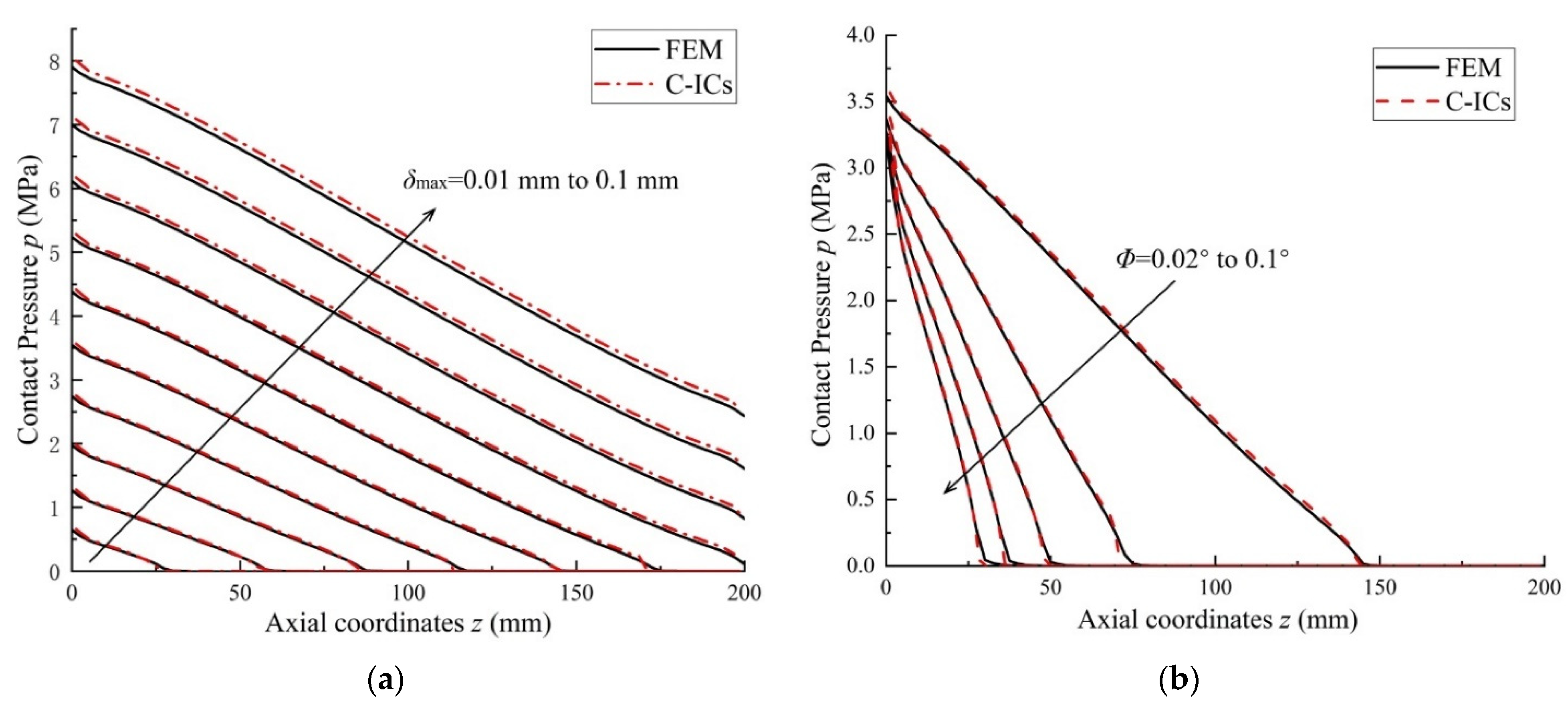
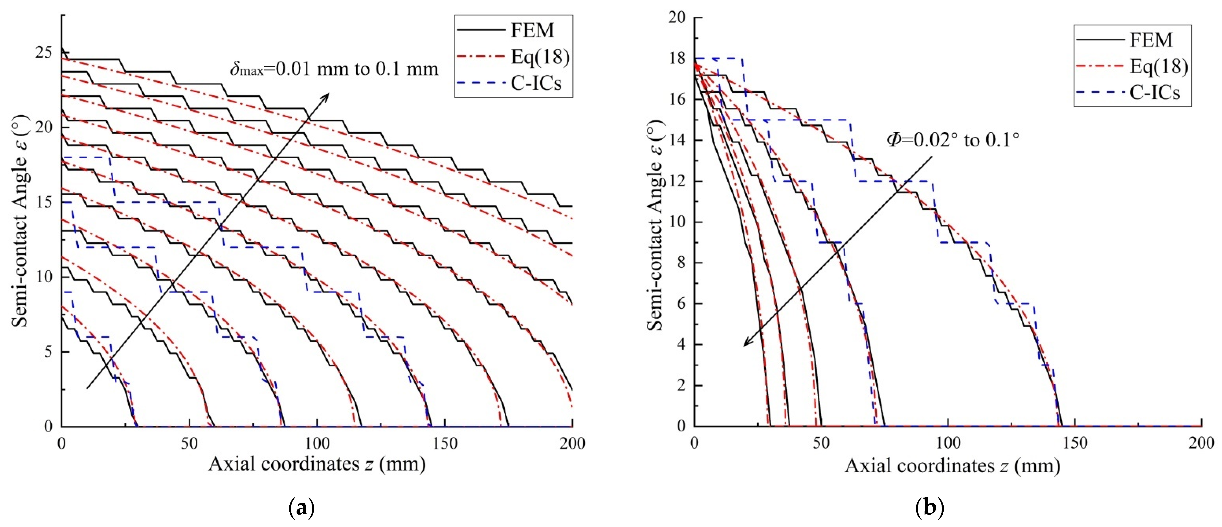
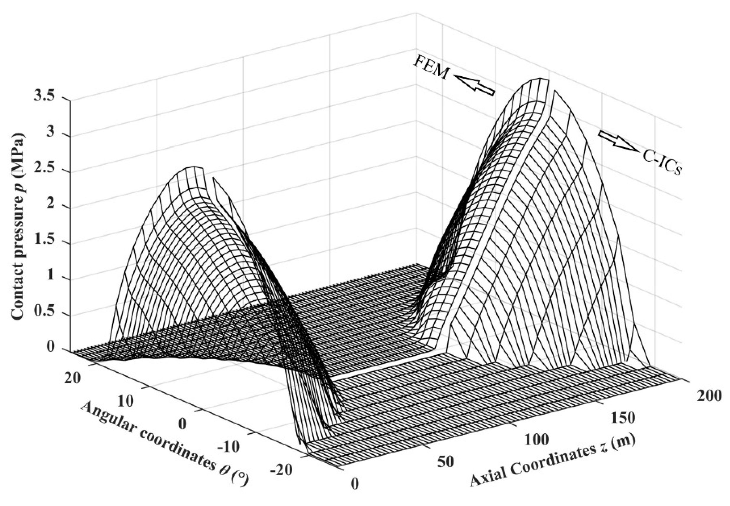
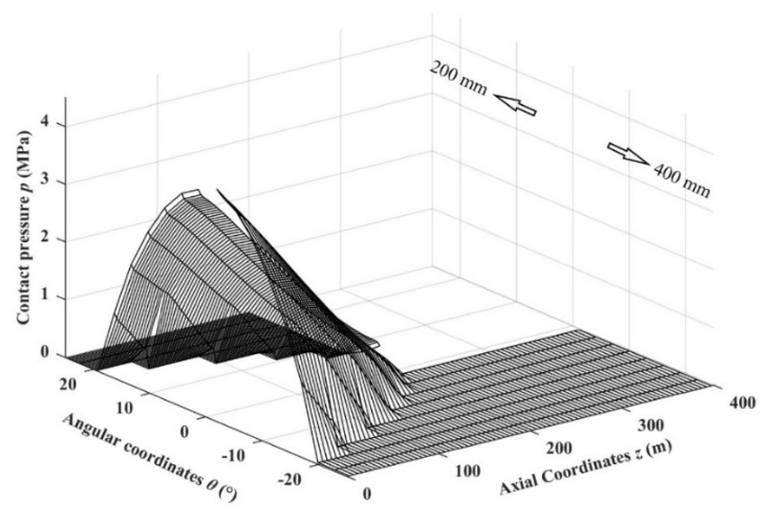
3.2. Contact Calculation of Misaligned Bearing

In the following studies, the C-ICs method was employed for the contact calculations of a single bearing with the non-aligned shaft. It was divided into two cases: the axis of the shaft is straight with an inclination angle, Φ; the axis is curved, as shown in Figure 2c,d. The FEM was used to verify its accuracy.

The maximum allowable Φ specified by the CCS rule is 0.02° [6]. However, this regulation is only for the static axis in the dock. When the ship is launched, the angle will change as the ship’s load changes. The maximum allowable mean pressure of the Thordon bearing is 0.5 MPa, given by the manufacturer. According to this value, it can be calculated that the maximum allowable bearing force is 20 kN, and the corresponding approachment δ_max when Φ = 0° is approximately 0.05 mm. The situation corresponding to Φ = 0.02° and δ_max = 0.05 mm was taken as the baseline condition for the case of a straight shaft.

Figure 9 is the FEM result of the radial displacement and the radial contact pressure of the baseline condition. It can be seen from Figure 9a that the contact area was located at the bottom and only occupied a small part of the inner surface of the bearing. The point of maximum contact pressure was located at the bottom of the left end, and the contact pressure varied in the axial and circumferential directions. The contact pressure in the non-contact area tended to 0 but was not equal to 0, which was caused by the anti-deformation phenomenon. The radial displacement distribution was similar to the radial stress distribution. The radial pressure was also large in places with high pressure.

The nodal contact pressure results of FEM were extracted and compared with the results of C-ICs to obtain Figure 10. The contact pressure at any point is represented as the height of the surface above the plane, while the contact area is the region under the doom. Although the FEM result was better than the mesh of the C-ICs result, the two results are symmetrical to the intermediate plane. There are some blanks in the C-ICs results near 0°, as each center point is used to represent the pressure value of the grid.

A comparison of contact pressure at the midplane of bearing between the C-ICs and FEM with different approachment and inclinations is shown in Figure 11. Good agreement could be observed between the two methods under all conditions. The contact pressure exhibited linear characteristics along the axial direction. This shows that the bearing pressure and the approachment are linear along the axial direction.

Figure 12 is the comparison of the boundary curve of the contact area. The result of Equation (18) agreed with the FEM result, while the boundary result of C-ICs was a jagged curve and had a deviation from the curve of Equation (18). As the grid center was used to judge whether the grid was in the contact area, the whole grid would be treated as a contact area once the grid center was in the boundary of Equation (18). The jagged curve would be close to the curve of Equation (18) by increasing the number of segments. The contact area of the C-ICs method only displayed a few specific situations due to the fact that as δ_max increased and Φ decreased, interference between the curves affected the observation.

In the case of a curved shaft, the bending moment was applied to the shaft ends. The maximum approachment was set to δ_max = 0.05 mm; the contact pressure comparison of FEM and the C-ICs method for the curved shaft situation is shown in Figure 13. The two results were also similar. It was proved that the proposed method is also applicable to bending situations. The results obtained after changing the amount of approachment and the degree of bending were similar to the results of the tilted straight shaft, so they are not discussed further here.

The time consumption comparison of the baseline condition is shown in

Table 3. Comparison of time consumption.

	FEM	C-ICs
Time consumption *	17 min	9 min

* Time consumption was calculated based on a computer with a dual-core 3.1 GHz CPU and 256 Gb RAM.

. The C-ICs method requires only half the time of FEM to obtain a similar result. In order to minimize the time of FEM, all pre-processing steps were programmed. Moreover, the relatively time-consuming factor of the C-ICs method is the calculation of the ICs factor, which takes approximately 8 min. The calculation time can be greatly shortened by storing the ICs factors in advance. The FEM analysis time is close each time, and it has higher requirements for computer hardware. Therefore, the C-ICs method has advantages in multi-condition analysis.

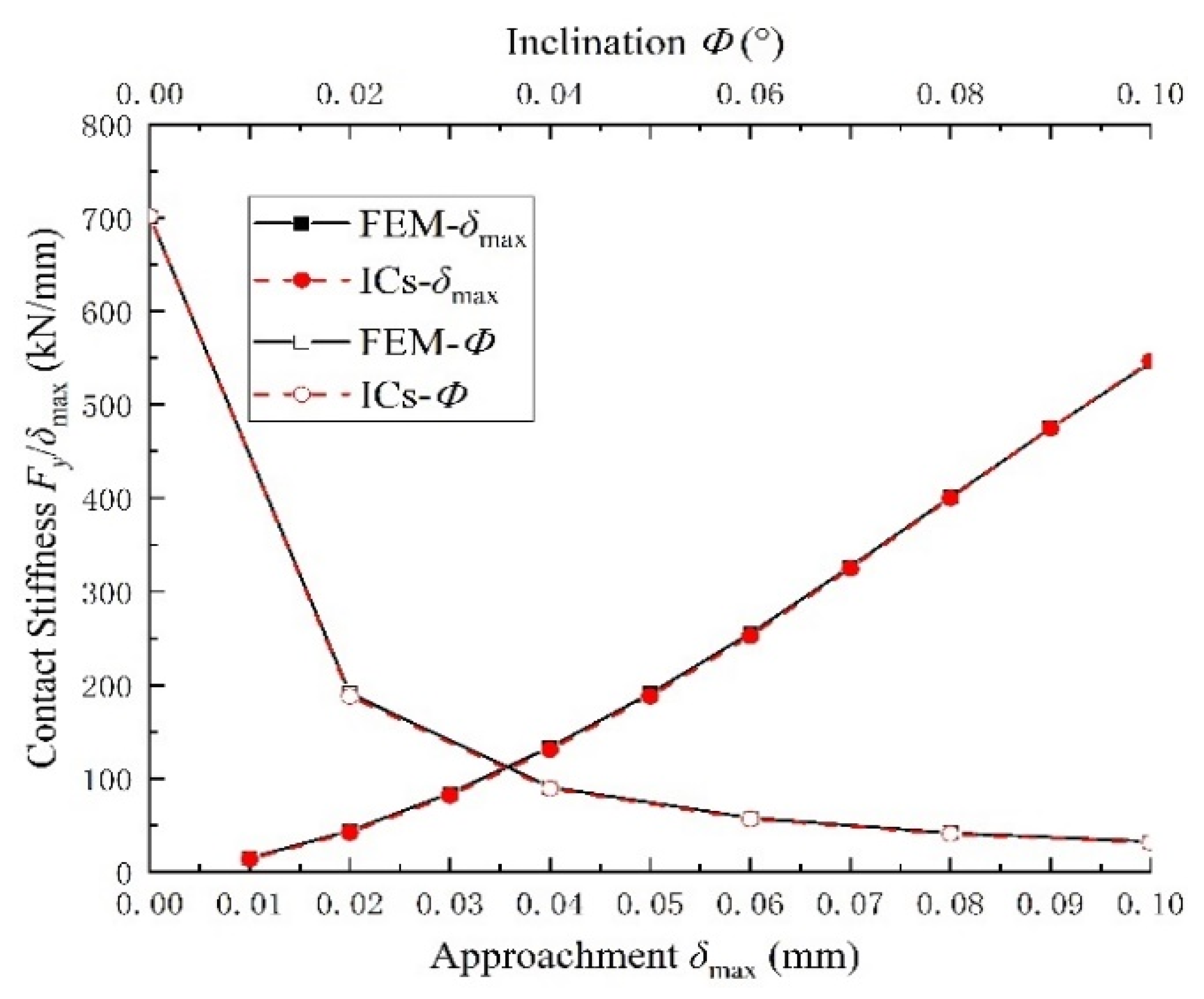
3.3. Influence of Misalignment on Journal Bearing Capacity and Contact Stiffness

The bearing capacity and contact stiffness are the critical parameters in the bearing’s static and dynamic analysis, respectively. One of the problems of large bearings is how to improve the bearing capacity. For ship shafting, the usual approach is to increase the length of the bearing. Figure 14 shows the bearing contact pressure distribution results with different lengths under baseline conditions and 20 kN load. It could be seen that the contact pressure changed slightly after doubling. The maximum contact pressure decreased from 4.03 MPa to 3.94 MPa as the extension bore part of the load. However, the original area still bore the main load, indicating that the increased length of 200 mm is not an effective contact area due to the misalignment. Thus, the bearing capacity did not improve concerning the maximum contact pressure as a failure criterion.

In the vibration problem analysis involving the elastomeric journal bearing, the contact stiffness of the bearing is necessary for input and is considered to be of particular value [15]. Figure 15 shows the contact stiffness values when the approachment and the inclination were changed, respectively. It can be seen that the contact stiffness increased with increasing approachment with a fixed tilt. Conversely, increasing the inclination angle reduced the contact stiffness. It is easy to explain this law by linking the contact stiffness with the contact area, as shown in Figure 12. A large contact area corresponds to large contact stiffness. During shaft operation, the deflection is constantly changing. Therefore, it is not appropriate to set the bearing contact stiffness to a fixed value.

4. Conclusions and Future works

The main conclusions can be drawn as follows:

(1)

The calculation of the cylindrical shell subjected to uniform internal pressure with different coefficient influence factors (ICs factor) obtained significantly different results, proving that the contact body’s geometric shapes and boundary conditions affect the ICs factor. The ICs factor shown in this article is suitable for cylindrical surface contact analysis;

(2)

The proposed method has similar accuracy in the contact pressure calculation of a misaligned elastomeric journal bearing with the FEM. Nevertheless, the time consumption is only half of the FEM and can be further reduced to 1/30^th by storing the ICs factor in advance;

(3)

The bearing misalignment influences the load-carrying capacity and the contact stiffness. The key to improving the load-carrying capacity is to increase the effective contact area. Additionally, the contact stiffness has the same changing trend as the contact area.

The investigation presented in this paper leaves some issues for future research, as discussed in the following:

(1)

The theoretical solution form of the cylindrical shell subjected to a concentrated force contains the first and second types of deformed Bessel functions, which are prone to data overflow during numerical processing and reduce accuracy. Finding other theoretical solutions with compact forms can further improve the method;

(2)

The non-alignment conditions of the bearings in this paper are assumed according to the rules. The work would be more meaningful if the actual propulsion shafting data could be obtained and input.

References

1. Choi, S.; Lee, J.; Park, J. Application of deep reinforcement learning to predict shaft deformation considering hull deformation of medium-sized oil/chemical tanker. J. Mar. Sci. Eng. 2021, 9, 767. [Google Scholar] [CrossRef]
2. Hirani, H.; Verma, M. Tribological study of elastomeric bearings for marine propeller shaft system. Tribol. Int. 2009, 42, 378–390. [Google Scholar] [CrossRef]
3. Lee, J.; Jeong, B.; An, T.H. Investigation on effective support point of single stern tube bearing for marine propulsion shaft alignment. Mar. Struct. 2019, 64, 1–17. [Google Scholar] [CrossRef] [Green Version]
4. DNV GL. Incomplete propeller immersion risk of propeller shaft bearing damage. Tech. Regul. News 2017, 1, 1–3. [Google Scholar]
5. ABS. Guidance Notes on ‘Propulsion Shafting Alignment’. Available online: https://ww2.eagle.org/content/dam/eagle/rules-and-guides/current/design_and_analysis/128_propulsionshaftalignment/shaft-alignment-gn-sept-19.pdf (accessed on 1 July 2021).
6. CCS. Part 3 Main and Auxiliary Machinery, Chapter 12 shaft vibration and alignment. In Rules for the Construction of Domestic Sailing Sea Vessels; CCS: Beijing, China, 2018. [Google Scholar]
7. Lloyd’s Register. Rules and Regulations for the Classification of Ships. Available online: https://www.lr.org/en/rules-and-regulations-for-the-classification-of-ships/ (accessed on 1 July 2021).
8. Johnson, K.L. Contact Mechanics; Press Syndicate of the University of Cambridge: New York, NY, USA, 1985; pp. 114–118. [Google Scholar]
9. Ciavarella, M.; Decuzzi, P. The state of stress induced by the plane frictionless cylindrical contact. I. The case of elastic similarity. Int. J. Solids Struct. 2001, 38, 4507–4523. [Google Scholar] [CrossRef]
10. Ciavarella, M.; Decuzzi, P. The state of stress induced by the plane frictionless cylindrical contact. II. The general case. Int. J. Solids Struct. 2001, 38, 4525–4533. [Google Scholar] [CrossRef] [Green Version]
11. Pereira, C.; Ramalho, A.; Ambrosio, J. Applicability domain of internal cylindrical contact force models. Mech. Mach. Theory 2014, 78, 141–157. [Google Scholar] [CrossRef]
12. Steven, G.P. A non-axisymmetric cylindrical contact problem. Int. J. Eng. Sci. 1977, 15, 95–103. [Google Scholar] [CrossRef]
13. Liu, C.; Zhang, K.; Yang, L. The compliance contact model of cylindrical joints with clearances. Acta Mech. Sin. 2005, 21, 451–458. [Google Scholar] [CrossRef]
14. Liu, C.; Zhang, K.; Yang, L. The FEM analysis and approximate model for cylindrical joints with clearances. Mech. Mach. Theory 2007, 42, 183–197. [Google Scholar] [CrossRef]
15. Lai, G.; Liu, J.; Liu, S.; Zeng, F.; Zhou, R.; Lei, J. Comprehensive optimization for the alignment quality and whirling vibration damping of a motor drive shafting. Ocean Eng. 2018, 157, 26–34. [Google Scholar] [CrossRef]
16. Hartnett, M.J. The analysis of contact stresses in rolling element bearings. J. Lubr. Tech. 1979, 101, 105–109. [Google Scholar] [CrossRef]
17. Lv, F.; Ya, N.; Rao, Z. Analysis of equivalent supporting point location and carrying capacity of misaligned journal bearing. Tribol. Int. 2017, 116, 26–38. [Google Scholar] [CrossRef]
18. Gong, J.; Jin, Y.; Liu, Z.; Jiang, H.; Xiao, M. Study on influencing factors of lubrication performance of water-lubricated micro-groove bearing. Tribol. Int. 2019, 129, 390–397. [Google Scholar] [CrossRef]
19. Timoshenko, S.P.; Goodier, J.N. Theory of Elasticity, 3rd ed.; McGraw-Hill: New York, NY, USA, 1970; pp. 366–368. [Google Scholar]
20. Yao, J.C. Long cylindrical tube subjected to two diametrically opposite loads. Aeronaut. Q. 1969, 20, 365–381. [Google Scholar] [CrossRef]
21. Shang, X.; Qiu, F.; Zhao, H.; Li, W. Ansys Advanced Structural Finite Element Analysis Methods and Sample Applications, 1st ed.; China WaterPower Press: Beijing, China, 2006; pp. 180–224. [Google Scholar]
22. Madenci, E.; Guven, I. The Finite Element Method and Applications in Engineering Using ANSYS, 2nd ed.; Springer: Boston, MA, USA, 2015; pp. 579–594. Available online: https://link.springer.com/book/10.1007/978-1-4899-7550-8 (accessed on 1 July 2021).
Figure 1. The excessively worn bearing.
Jmse 10 00141 g001
Figure 2. Contact diagram of the bearing: (a) the elastomeric journal bearing is installed on the steel bushing; (b) schematic diagram of the cross-section; (c) tilted shaft in contact with the bearing; (d) curved shaft in contact with the bearing.
Jmse 10 00141 g002aJmse 10 00141 g002b
Figure 3. Schematic diagram of the ICs method.
Jmse 10 00141 g003
Figure 4. Cross-sectional schematic diagram of the geometric boundary of the aligned bearing.
Jmse 10 00141 g004
Figure 5. Flow chart of the numerical calculation.
Jmse 10 00141 g005
Figure 6. The finite element model of single bearing contact. (a) Global view of the model. (b) Cross-sectional view.
Jmse 10 00141 g006
Figure 7. Comparison of different influence coefficient factors: (a) the displacement distribution of cylindrical tube subjected to a concentrated force (C-ICs factor); (b) the displacement distribution of half-space plane subjected to a concentrated force (HS-ICs factor); (c) comparison of displacement distribution at z = 0.
Jmse 10 00141 g007aJmse 10 00141 g007b
Figure 8. Displacement distribution of a cylindrical shell under unit uniform internal pressure.
Jmse 10 00141 g008
Figure 9. FEM results for straight shaft when Φ = 0.02° and δmax = 0.05 mm: (a) result of contact pressure; (b) result of radial displacement.
Jmse 10 00141 g009
Figure 10. Comparison of results between FEM and the C-ICs method when Φ = 0.02° and δmax = 0.05 mm.
Jmse 10 00141 g010
Figure 11. Comparison of axial contact pressure: (a) the approachment δmax changed from 0.01 mm to 0.1 mm; (b) the inclination Φ changed from 0.02° to 0.1°.
Jmse 10 00141 g011
Figure 12. Comparison of contact area: (a) The approachment δmax changed from 0.01 mm to 0.1 mm; (b) the inclination Φ changed from 0.02° to 0.1°.
Jmse 10 00141 g012
Figure 13. Comparison of results between FEM and the C-ICs methods for a curved shaft contact with the bearing when δmax = 0.05 mm.
Jmse 10 00141 g013
Figure 14. Contact pressure comparison with different bearing lengths.
Jmse 10 00141 g014
Figure 15. Contact stiffness of the bearing with different approachment and inclination.
Jmse 10 00141 g015