Abstract
Ducted propeller is a kind of special propeller widely used in unmanned underwater vehicles, its flow characteristics and hydrodynamic noise are very important for marine environmental protection and equipment concealment. The hybrid techniques based on the acoustic analogy theory are adopted in the present study to calculate the unsteady flow field and sound field characteristics of a ducted propeller. The full scale flow filed and hydro-acoustic sources of the propulsion system are simulated by Detached-Eddy computational fluid dynamics (CFD) method. Hydrodynamic noise are calculated by FWH equation based on the CFD results. The frequency domain and directivity of sound pressure level at different sound field monitoring points are analyzed at four navigational speeds. The results show that the navigational speed that is in the inflow condition of the ducted propeller play important roles in the flow structure and underwater radiated noise. Under the fixed impeller rotational speed, the propulsion efficiency of ducted propeller increases first and then decreases with the raise of navigational speed. The maximum errors of thrust and power between simulation and experiment values are 0.5% and 0.1% respectively, which means that the adopted DES numerical simulation method has high credibility in calculating the acoustic source. At impeller rotational speed of 2000 r/min, the best state of flow field distribution is at the navigational speed of 1.54 m/s, which is corresponding to the highest propulsion efficiency condition. The propeller noise presents dipole characteristic in all working conditions, and at the obvious blade passing frequency, multiple characteristics are presented; most of the noise contribution is also concentrated below four times of the blade passing frequency. The total sound pressure level of the hydrodynamic noise is the smallest at the optimal efficiency condition (the navigational speed is 1.54 m/s). At high navigational speed, the low frequency characteristics below blade passing frequency increase and the amplitude becomes larger. This indicates that the component of turbulent noise becomes more important with the increase of navigational speed. The research focuses on analyzing the relationship between the energy loss of the ducted propeller wake field and the noise level, and it is found that the vortex at the tail makes a certain contribution to the noise. The research conclusions could provide some reference for the acoustic performance evaluation and noise reduction optimization of ducted propeller design as well as the improvement of UUV stealth performance.
1. Introduction
With the attention paid to marine development, the interest in the underwater field development of specific tools for the sub-sea inspection is increasing. Because it is suitable for long-period and large-scale investigation tasks, unmanned underwater vehicles (UUV) technology has developed rapidly [1,2]. In general, UUV mainly includes remotely operated vehicles (ROV) and autonomous underwater vehicles (AUV). Due to the simple structure and convenient operation characteristics, the electric ducted propeller is widely used as the propulsion device of UUV. It is also an important energy consumption equipment and a noise source for UUV in reconnaissance, intelligence collection and ocean exploration [3]. Since the motor and controller can be placed into the cabin, hydrodynamic noise is the main source of the ducted propeller [4]. Therefore, in-depth study on the acoustic characteristics of the ducted propeller under different working conditions is of great significance to put forward effective noise reduction measures and improve the operation ability of UUV.
The ducted propeller is developed on the basis of propeller, which adds an annular duct with airfoil section. For years research has been performed to improve the performance of the existing propellers and to design new propellers according to the market needs [5]. Gaafary et al. [6] introduced a procedure to select the optimum characteristics of B-series marine propellers while considering the limitation of both material strength and cavitation issues. Mirjalili et al. [7] employed the multi-objective particle swarm optimization (MOPSO) method to optimize the shape of marine propellers in order to maximize the propeller efficiency and minimize cavitation issues. With the development of computer technology, numerical research has gradually become an important means to predict and optimize the performance of propellers. Gaggero et al. [8] proposed an optimization process for high-speed propeller by combining a fast and reliable Boundary Elements Method (BEM), a viscous flow solver based on the RANSE approximation, a parametric 3D description of the blade and a genetic algorithm. Normally, the principal way to reduce the noise of propeller is to improve the cavitation performance of propeller. Due to the addition of the duct, the impeller design of ducted propeller is between the propeller and the pump, and the cavitation performance is greatly improved. In the field of shape optimization of underwater vehicles and rotating machinery design, researchers can numerically optimize its geometric parameters with the rapid development of computational fluid dynamics (CFD) technology to ensure that the propeller can operat under non cavitation conditions [9,10].
Due to the need to collect signals, ducted thrusters often operate at mooring and low navigational speed. The hydrodynamic noise radiated by the propeller under non cavitation is one of the main factors that interfere with the working ability of UUV. Based on Lightill’s aeroacoustic theory [11], flow induced noise is mainly composed of the fluid solid interaction and turbulence hydroacoustic. Therefore, accurate prediction and analysis of the detailed flow field is the premise of acoustic characteristic predicting. Unlike open propellers, there is a tip clearance between the nozzle and the blade tip of a ducted rotor. Oweis and Ceccio [12] observed a primary tip-leakage vortex that interacts with a secondary trailing edge vortex from instantaneous flow fields measured by a Planar Particle Imaging Velocimetry (PIV) technique in the tip region of a ducted marine propulsor. Along with the physical experimental studies, the application of CFD for the understanding of the flow characteristic has also been considered [13,14,15]. Qiu et al. [16] adopted the SST k-ω turbulence model and the sliding mesh technology to simulate the exciting force and hydrodynamic of a pump-jet propulsor in different oblique inflow angle. They found that the variation of the pulsating pressure becomes greater as the closer to the blade’s tip inside the rotor domain. However, both the vortex lattice method and the MRF method cannot provide accurate wake fields. Kumar and Mahesh [17] studied the wake of a five-bladed marine propeller at design operating condition by using large eddy simulation (LES). In order to avoid the limitation of the grid number, Zhang et al. [18] numerically investigated the wake dynamics and instabilities of a ducted propeller by employing a hybrid RANS/LES model and the transient sliding mesh approach, the spectral analysis of the simulation indicates a much broader and more energy intensive frequencies for the zero inflow condition. For the numerical simulation of hydroacoustic sources and the noise propagation, the use of hybrid techniques allows the expensive CFD calculation to be restricted to the sources regions, whereas noise propagation is handled by simplified flow equations and acoustic analogies et al. Ebrahimi et al. [19] developed a numerical code based on the Ffowcs Williams-Hawkings(FWH) analogy model to calculate flow induced noise by using the velocity and pressure distribution around the propeller. Then, a genetic algorithm was used to optimize the hydro-acoustic and hydrodynamic performance of propellers. The experimental results show that the method is successful in engineering application. Wang et al. [20] proposed a hybrid method, in which the FWH analogy is coupled with the Boundary Element Method (BEM)approach, to study the sound field properties of non-cavitating marine propellers under uniform and non-uniform inflow conditions. Yang et al. [21] analyzed the fluctuating noise sources of the full-scaled waterjet by coupling Scale-Adaptive Simulation (SAS) of periodic pulsating pressure on blades with BEM for the acoustic field. In view of the importance of the incoming flow to the waterjet performance and noise, numerical self-propelled tests of the full-scaled trimaran–waterjet system using the k-ε explicit algebraic Reynolds stress turbulent model with rotation curvature correction were completed to output the non-uniform inflow. The above research shows that the incoming flow—that is, the navigational speed of the UUV—has a great impact on the noise characteristics of the propeller. But they didn’t analyze the reason for the noise change.
In the present study, the hybrid techniques based on the combining of CFD and FWH are adopted to numerically calculate the unsteady flow field and sound field characteristics of a ducted propeller. The flow field in the rotating region of the impeller and wake vortex structure of the propeller are analyzed by entropy generation. Additionally, the hydro-acoustic sources’ contribution from the flow field of the ducted propeller to total noise under different navigational speed are analyzed.
2. Research Object and Methodology
2.1. Structural Parameters of the Ducted Propeller
The ducted propeller studied in this paper is shown in Figure 1, and is mainly composed of motor, impeller and duct. The motor drives the impeller to rotate through the shaft, which forms thrust and provides a power source for the UUV. In order to obtain better efficiency and thrust performance, the impeller combines the design theory of the pump and the propeller. There are no bracket at the front and back of the impeller, but four cylinders to support the duct. The main geometric parameters of hydraulic components are as follows: the inlet diameter of the duct is 105.5 mm, the motor hub diameter is 48 mm, the outlet diameter of the duct is 84.5 mm, the total length of the duct is 54 mm, the hub ratio is 0.2, the impeller diameter is 80 mm, the number of impeller blades is 3, the length of impeller flange airfoil is 31.3 mm, the length of impeller hub airfoil is 17.5 mm.
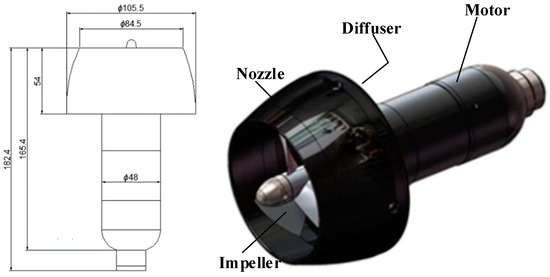
Figure 1.
Structure and the main size of the studied ducted propeller.
2.2. Experimental Support
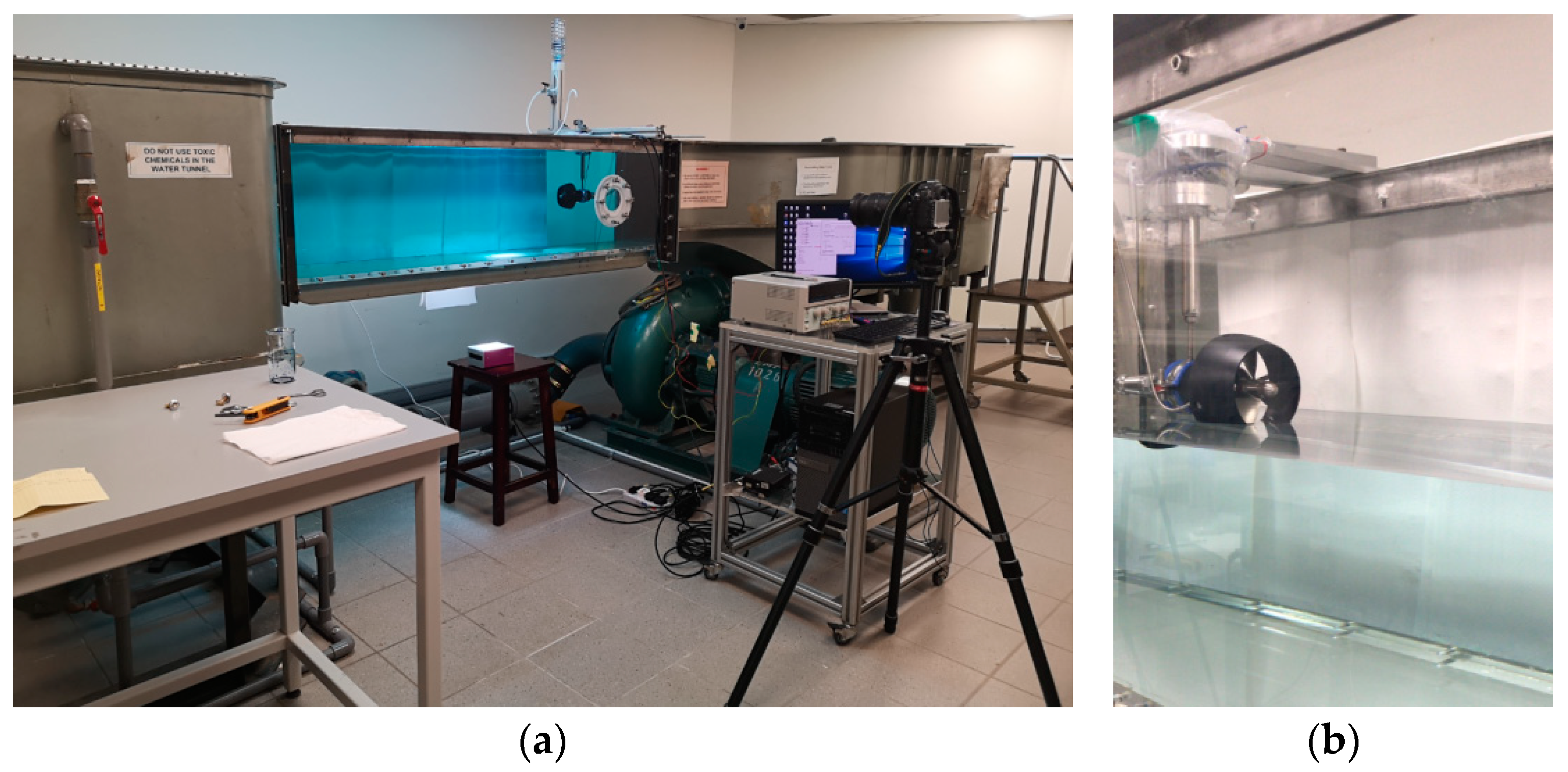
The open water experiments are processed on the built test rig, as shown in Figure 2. The test loop includes a steady flow water tank, a transparent experimental section, a return water tank, a circulating pump, a water inlet pipeline and a water discharge pipeline. The circulating pump can change the flow rate of water in the transparent experimental section, which simulate different navigational speed of the ducted propeller. The ducted propeller is hoisted in the transparent experimental section through a designed fixture, and the motor is supplied with 24 V DC power by GWINSTEK GPS-3303. The rotational speed and steering are controlled by a PWM regulator, which can read the rotational speed of the ducted propeller through PWM, and its rotational speed measurement accuracy is 0.25%. A six-degree-of-freedom force sensor is placed inside the fixture, and its measurement accuracy is 0.1%. Combined with the NI 6343 acquisition card and the LabView data acquisition program, the thrust of the ducted propeller is measured. The input power of the motor can be measured by the power supply, and the reading error of the DC power supply is 0.01 W. By combining this with the motor efficiency (88%) provided by the manufacturer, the propulsion efficiency of the ducted propeller can be obtained, as shown in Equation (1).

Figure 2.
Test rig and the ducted propeller installation. (a) Test rig; (b) Ducted propeller installation.
By injecting pigment and bubbles at the pump inlet and illuminating the jet area with a laser headlamp, the visualization experiment of jet flow pattern was carried out. Photos and videos were collected by camera.
Before the open water experiments, the six-degree-of-freedom force sensor was statically calibrated, and the standard weights were used for three repetitions of loading. In the same day, six repeated measurement experiments in open water were carried out at 19 different rotational speeds of the ducted propeller. The same water isolating time was used throughout the experiment. The zero point was collected before each test to ensure that the test system, testers and test conditions were completely consistent and meet the repeatable measurement conditions.
According to the results of 6 repeated open water experiments, the standard deviations of thrust and power of the ducted propeller are 0.26% and 0.34%. Then, by using the Bessel formula the standard uncertainty of the thrust and power measurement repeatability can be obtained, which are 0.29% and 0.41%, respectively.
2.3. Numerical Methodology of the Hydrodynamic Noise
2.3.1. Governing Equation
The full scaled flow conditions of the ducted propeller propulsor flow field follow the law of conservation of mass, momentum, and energy. Because the rotating speed is not high, the surface of the water cannot form an entrainment vortex with sucking air. Thus, the fluid properties are the only single water medium in our calculations, and these properties are that it is in-compressible and presents no heat exchange. The governing equations of the three-dimensional flow field which are named unsteady Reynolds Averaged Navier-Stokes equations that can be written as the mass and momentum conservation in the following tensor form:
2.3.2. Turbulence Model
In general, the two-equation eddy viscosity turbulence model such as k-ε model and k-ω are mostly used in engineering application. Menter [22] proposed the SST turbulence model by combining the advantages and characteristics of these two- equation eddy viscosity models. However, the hydrodynamic noise of ducted propeller also contains turbulent noise, but the Reynolds average equation averages the stress term. So, the hybrid RANS/LES model is more suitable for solving the acoustic term of complex flow field. Si et al. [23] developed a hybrid numerical method to predate the radiated noise characteristics of the multistage centrifugal pump, which is based on detached eddy simulation (DES) of the flow field and finite element acoustic calculation. The turbulence model for our numerical simulation is DES, which could capture the detailed flow information near the surface of the impeller and duct as the hydraulic exciting force. Together with the calculated wake hydro-acoustic, noise sources are used to process the next underwater radiated noise simulation.
The DES method is a modification of the RANS model in which the model switches to a sub grid scale formulation in regions fine enough for LES calculations, which calculates the sound source information and simultaneously cuts down the cost of the computation.
It is initially formulated for the Spalart–Allmaras model, which is expressed as:
where the variables that represent turbulent motion are the quantities directly solved by the S-A equation. The relationship with the motion viscosity coefficient is defined as:
where fv1 is a dimensionless function defined as:
where v is an expression of the molecular viscosity generation term expressed as:
where S is the absolute value of vorticity, and fv2 and fv3 express dimensionless functions, which are respectively expressed as:
fw is expressed as:
The constant value is evaluated as:
The DES method is based on the S-A model which replaces the feature-length dw as:
where represents the maximum grid distance, CDES = 0.6.
The default value of the software is adopted in the article. The size of the characteristic length is related to the scale of the grid, and the DES method is an S-A model of the LES simulation.
2.3.3. Acoustic Simulation Methodology
The most popular calculation approach is the hybrid method, combining an incompressible hydrodynamic solver and the Ffowcs Williams-Hawkings(FWH) acoustic analogy [24]. The FW-H equation is essentially an inhomogeneous wave equation that can be derived by manipulating the continuity equation and the Navier-Stokes equations. It clearly explains the three aerodynamic sound sources of rotor sound from the physical mechanism: turbulent sound source (quadrupole), rotor surface pulsation force sound source (dipole) and aerodynamic sound source (monopole) caused by rotor motion. These three correspond to turbulence, pulsation force and rotor thickness, respectively. The FW-H equation can be expressed as:
where is the fluid velocity component in the direction, is the fluid velocity component normal to the surface , is the surface velocity component normal to the surface, is the far-field sound speed, t is the time, is the Dirac delta function, is the Heaviside function, and is the sound pressure at the far field ().
denotes a mathematical surface introduced to embed the exterior flow problem () in an unbounded space, which facilitates the use of generalized function theory and the free-space Green function to obtain the solution. The surface () corresponds to the source surface, and can be made coincident with a body surface or a permeable surface off the body surface. is the unit normal vector pointing toward the exterior region (), and is the Lighthill stress tensor, expressed as:
is the compressive stress tensor. For a Stokesian fluid, this is expressed by:
3. Simulation Modeling
3.1. Computing Domain and Meshing
Consistent with the test, the full scaled calculation domain of the ducted propeller is set as the cuboid area shown in Figure 3. The total length of the cuboid is 26D (D is the impeller diameter), its cross section is square and its size is 8D × 8D. The distance from the inlet of the fluid domain to the impeller is 10D, and the distance from the outlet to the impeller is 16D. The calculation domain is divided into three parts: outflow field fluid domain, conduit fluid domain and impeller fluid domain.
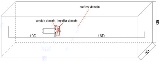
Figure 3.
Computing domain.
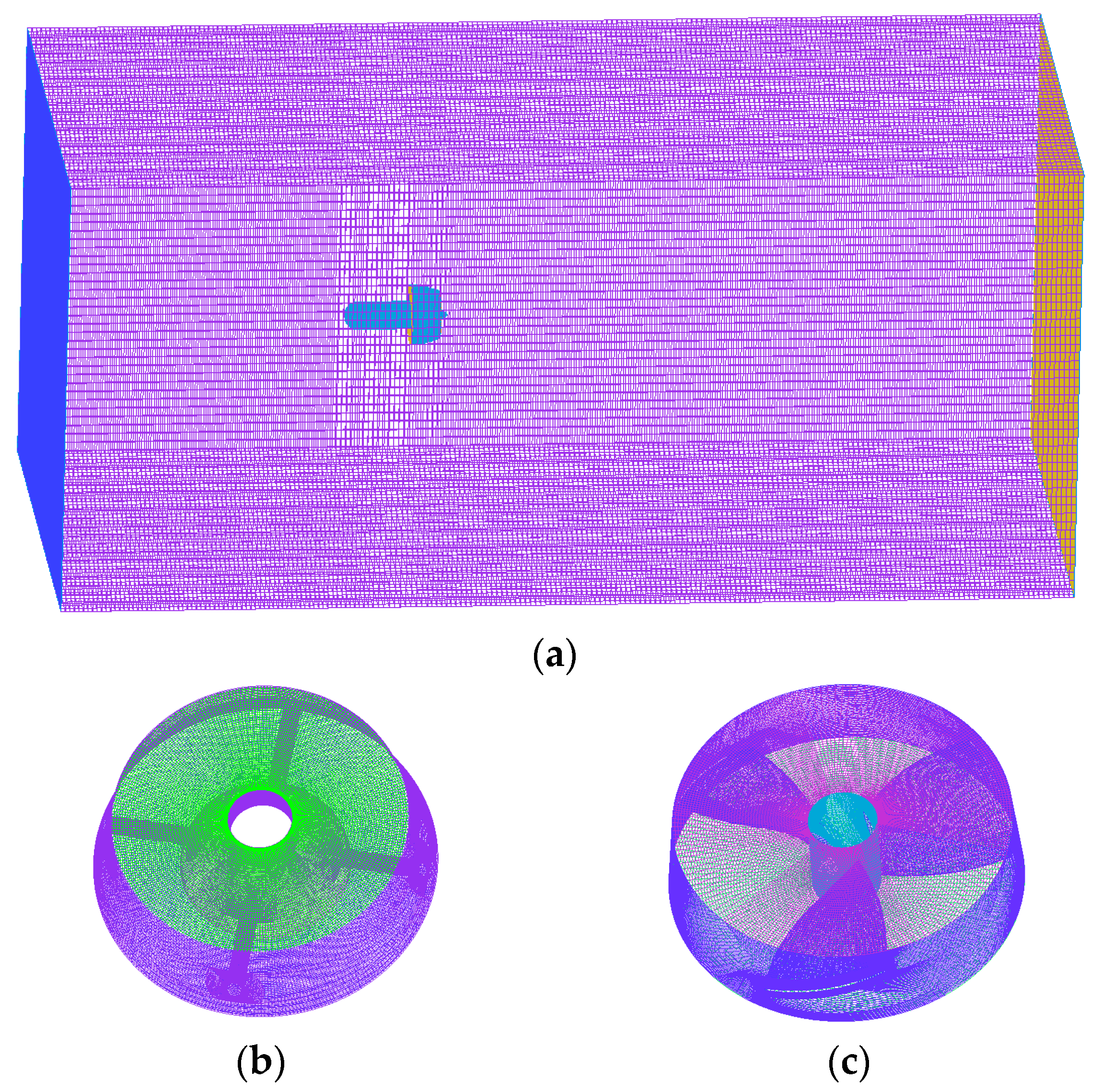
As shown in Figure 4a, the structured grid is applied for meshing the full scale computational domains by using ANSYS ICEM version 17.2 (ANSYS, Inc., Commonwealth of Pennsylvania, Harrisburg, PA, USA). A special refinement is applied around the blades hub, tip clearance, and wake area to improve the accuracy of the simulation. Boundary layers are added to all solid surfaces to ensure that the maximum non-dimensional wall distance y+ meets the selected turbulence model, as shown in Figure 4b,c.
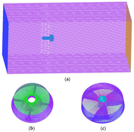
Figure 4.
Mesh of the computing domain. (a) Viscous entropy generation; (b) Mesh of the duct domain; (c) Mesh of the impeller domain.
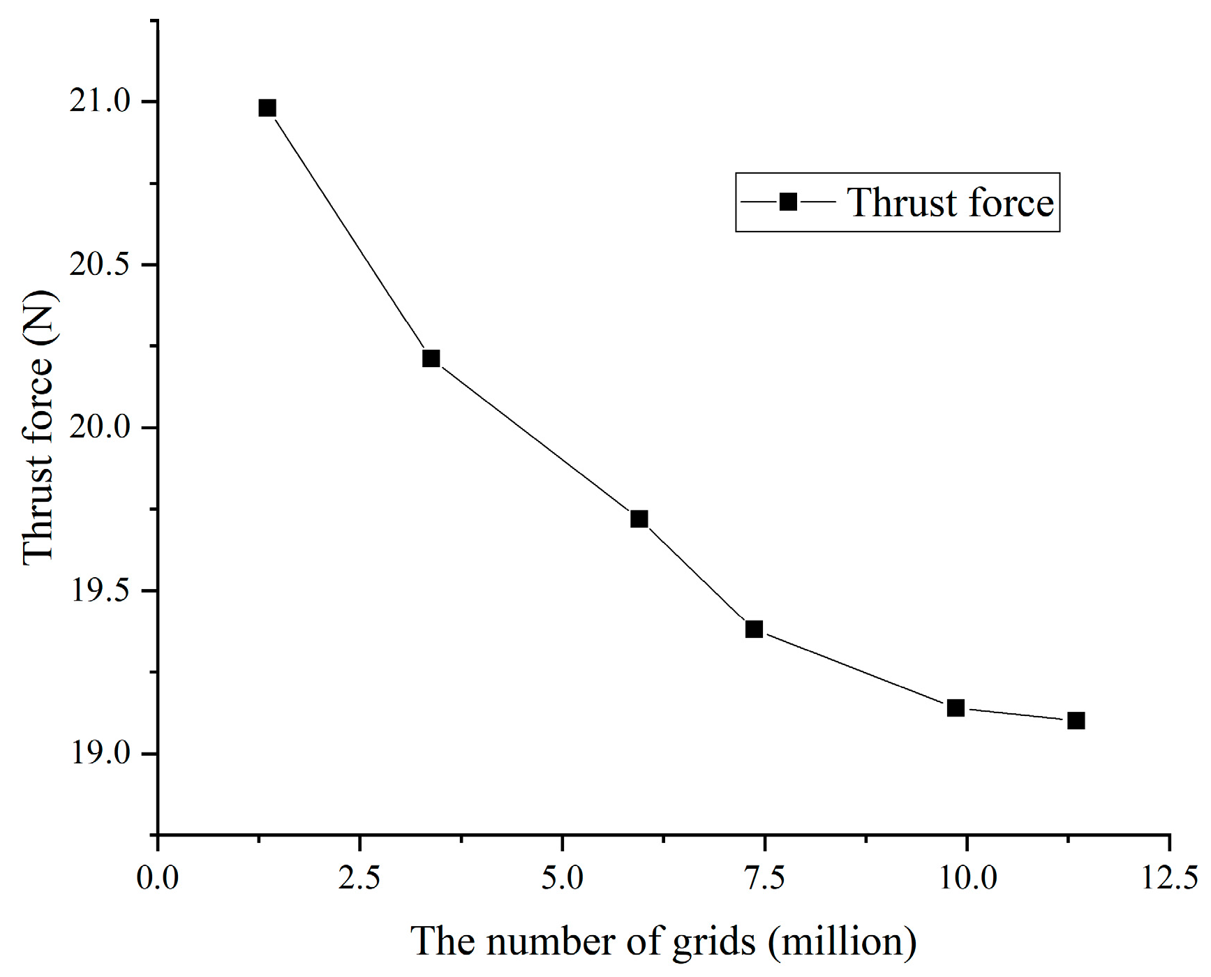
In addition, six groups of computational grids have been used for mesh independence analysis. The thrust of ducted propeller is taken as the target, its definition the relevant calculation boundary conditions are introduced in the next section. As can be seen in Figure 5, the thrust value changes within 1% after the number of grids reaches 9.88 million. Therefore, the total element number is chosen as 9,880,530 by considering the simulation accuracy and efficiency.
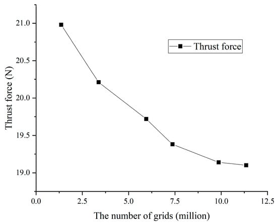
Figure 5.
Mesh independence analysis.
3.2. Boundary Conditions
The pre-converged steady flow field (based on the SST turbulence model) obtained is accepted as the initial condition followed by the unsteady simulation (based on the DES model). All simulations are processed by software ANSYS Fluent version 17.2 (ANSYS, Inc., Commonwealth of Pennsylvania, USA). The fluid medium is set as water at 25 °C. The inlet boundary is set as the velocity inlet and the outlet boundary is set as the pressure outlet with total pressure of 1atm. The inlet turbulence intensity is set to 5% of the initial value in the fluent software [25]. The walls around the cuboid, blades and the duct surface are set as non-slip walls. The impeller domain is set as rotating, which is rotates around the z-axis. While the outer basin and duct domain are set as stationary, and sliding grid interface are used to connect the different domains. The RMS residual is set to 10−4 as the standard for the convergence of the iterative calculation. In general, the final accuracy of an unsteady simulation is a function of the time step. It would significantly increase the calculation time if we set a small time step. The courant number defined by Equation (14) is always used as a criterion to judge whether the time step satisfies the periodic numerical simulation:
where L is the smallest size of the grid, v is the main flow velocity and is the time step. The maximum v is below 12 m/s, and L is more than 0.02 mm according to the ducted propeller geometry and grid information. The simulation set the time step as 1.0 × 10⁻⁴ s and the total time as 0.5 s. Then, the calculated maximum is 60, which satisfies the time step independence. The FW-H model was selected as the acoustic model for hydrodynamic noise calculation.
The calculations are carried out under four navigational speeds, which set the inflow velocity as 0 m/s (mooring state), 0.37 m/s, 1.54 m/s and 2.057 m/s.
4. Results Analysis
4.1. Performance Analysis of Ducted Propeller
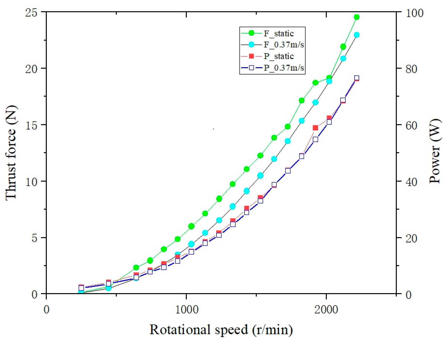
The comparison of the test thrust and power of studied ducted propeller under two flow states is shown in Figure 6. It can be seen that the thrust of the propeller in the mooring state is always greater than that at the speed of 0.37 m/s at all impeller rotational speeds. This might be because the ducted propeller has a smaller flowrate under the mooring state, and the rotating impeller brings about a bigger lift to the flow. The thrust is at its maximum at the mooring state with the biggest impeller rotational speed. In addition, the power of the ducted propeller in the two states is mostly the same at different impeller rotational speeds. The exception is when the rotating speed is 800 r/min to 1500 r/min, the power in the mooring state is slightly higher than that it is in 0.37 m/s speed navigation.
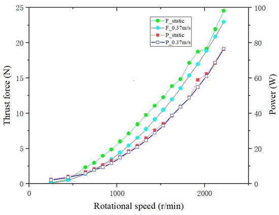
Figure 6.
Thrust and power of the ducted propeller at different impeller rotational speed.
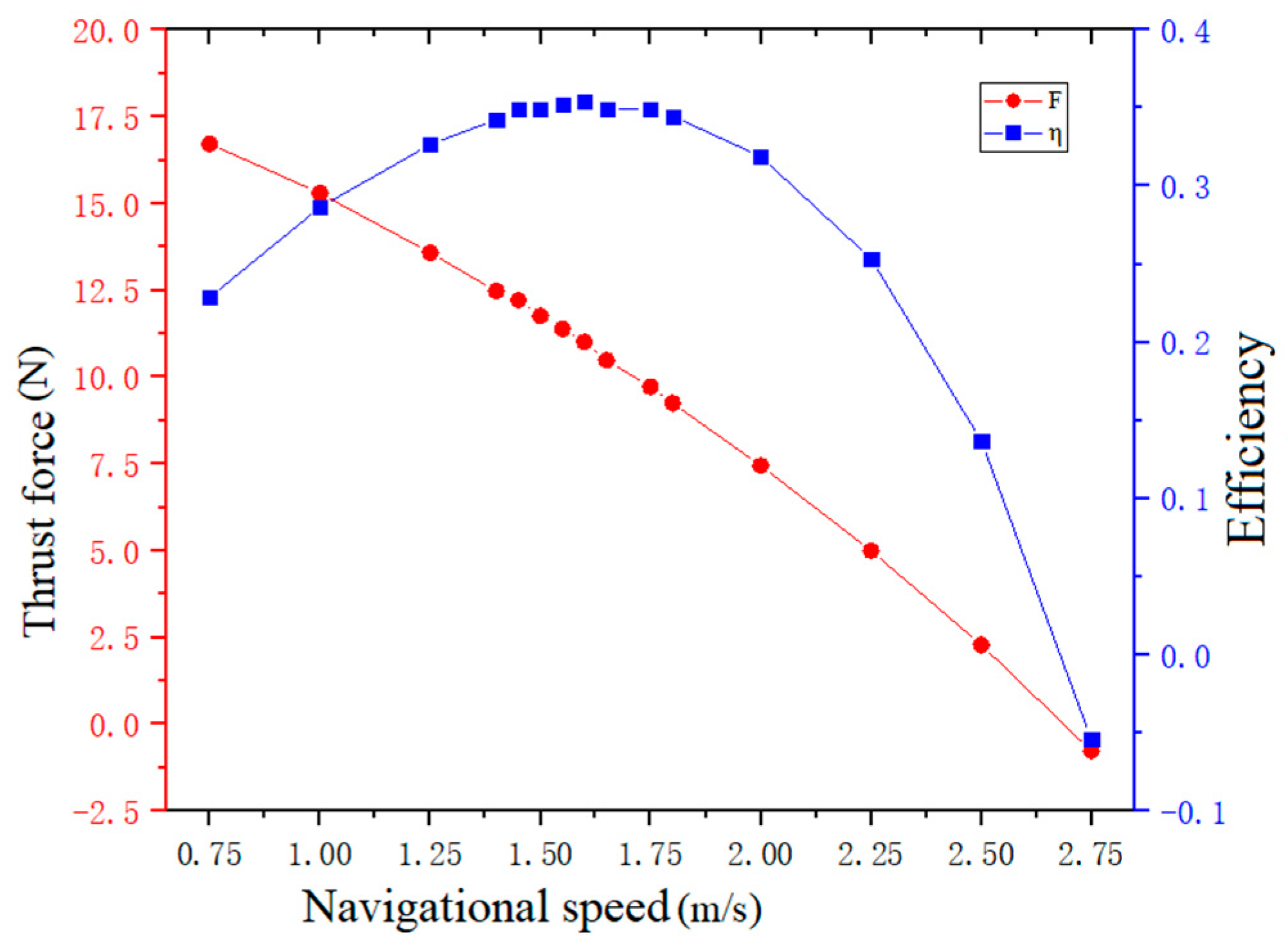
The performance curves of the ducted propeller under the impeller rotating speed of 2000 r/min are shown in Figure 7. It can be seen that the thrust of the propeller decreases gradually with the increase of the navigational speed. The propulsion efficiency increases first, reaching the highest point when the navigational speed is about 1.54 m/s, and then it decreases when the navigational speed accelerates further. The trend is basically consistent with the existing theory of the ducted propeller.
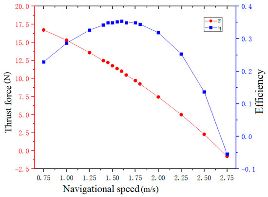
Figure 7.
Performance curves of ducted propeller at impeller rotational speed at 2000 r/min.
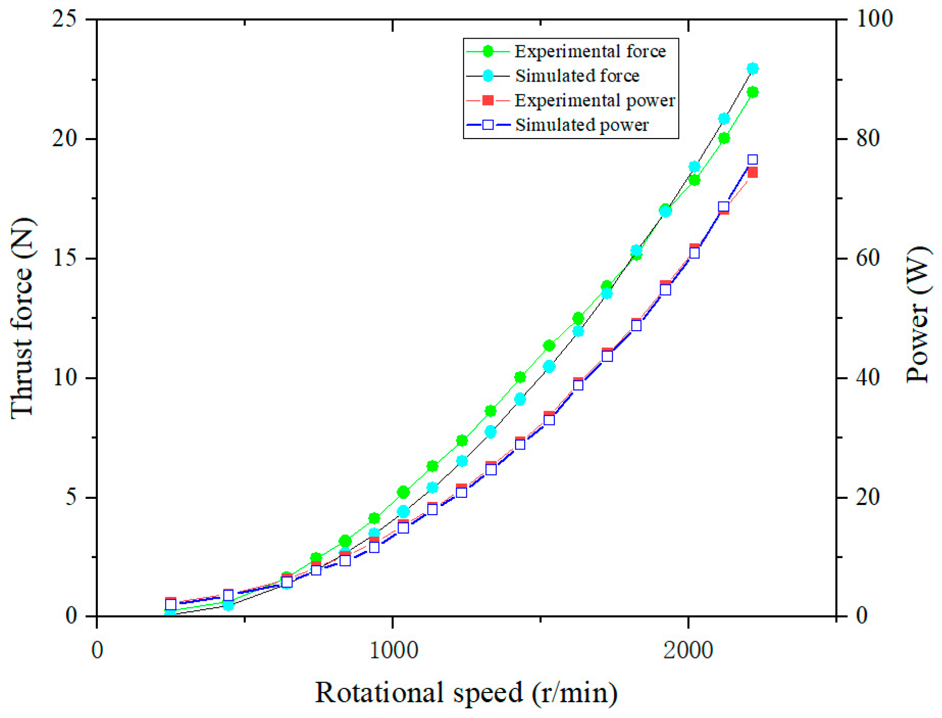
In order to verify the accuracy of the numerical calculation results, the performance results of the ducted propeller are compared at navigational speed of 0.37 m/s under different impeller rotational speeds, as shown in Figure 8. In post numerical simulation, the thrust and power of the ducted propeller are obtained by the following formula.
where expresses the inflow velocity, expresses the outlet velocity, Q expresses the flowrate passing through the duct, expresses the radial velocity at the inlet overflow section of the duct, and expresses the area of the inlet overflow section.
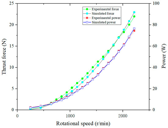
Figure 8.
Comparison of performance results between test and numerical calculation.
Seen from the figure, the numerical calculation results are consistent with the data trend of the test ducted propeller results. The maximum errors of thrust and power are 0.5% and 0.1%, respectively, which meets the error requirements of the calculation model. The geometric model, numerical method, meshing and boundary condition settings used in this statement are reasonable, and the numerical calculation results are reliable.
4.2. Flow Field Analysis
4.2.1. Velocity Distribution at Different Navigational Speeds
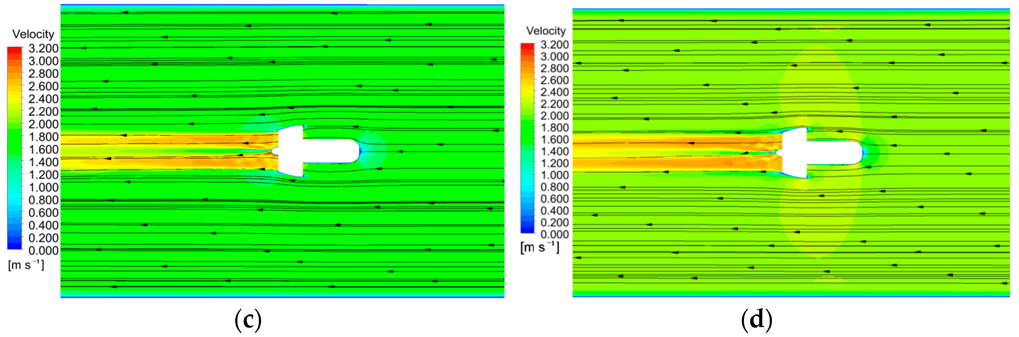
The velocity streamline diagram of the ducted propeller full-scaled flow field under different navigational speed conditions when the impeller rotational speed is 2000 r/min is shown in Figure 9. It can be clearly seen in the working process of the ducted propeller that the fluid enters the thruster through the inlet of the duct, works under the lift of the impeller and with the velocity increasing, and finally ejects from the tail nozzle to mix with the low-velocity fluid at the outlet of the propeller flow field. When the navigational speed is low, a pair of symmetrical vortices with opposite rotation directions are formed on both sides of the wake area. The symmetrical vortices formed in the mooring state are closer to the duct outlet, and the mainstream area of the velocity flow field is shorter. With the increase of the distance, the influence of the impeller hub gradually increases, and finally it bifurcates into two streams of fluid at the end of the velocity mainstream area. However, as the navigational speed increases, the pair of vortices in the wake area gradually disappear and the flow lines become more layered. This indicates that the efficiency of the propellers changes as the navigational speed increases.
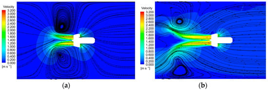
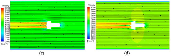
Figure 9.
Velocity distribution diagram of different navigational speed with 2000 r/min impeller rotational speed. (a) 0 m/s; (b) 0.37 m/s; (c) 1.54 m/s; (d) 2.057 m/s.
4.2.2. Vorticity and Entropy Distribution at Different Navigational Speeds
Among the second generation vortex identification methods, the Q criterion is the most widely used vortex identification method. The Q-expression can be written as:
where represents the square of the norm of matrix B, which is equivalent to the sum of the squares of all elements of matrix B. And matrix A and matrix B are, respectively, the symmetric tensor and anti-symmetric tensor of velocity gradient, which are defined as:
where T represents the transpose of the matrix. The velocity tensor is defined as:
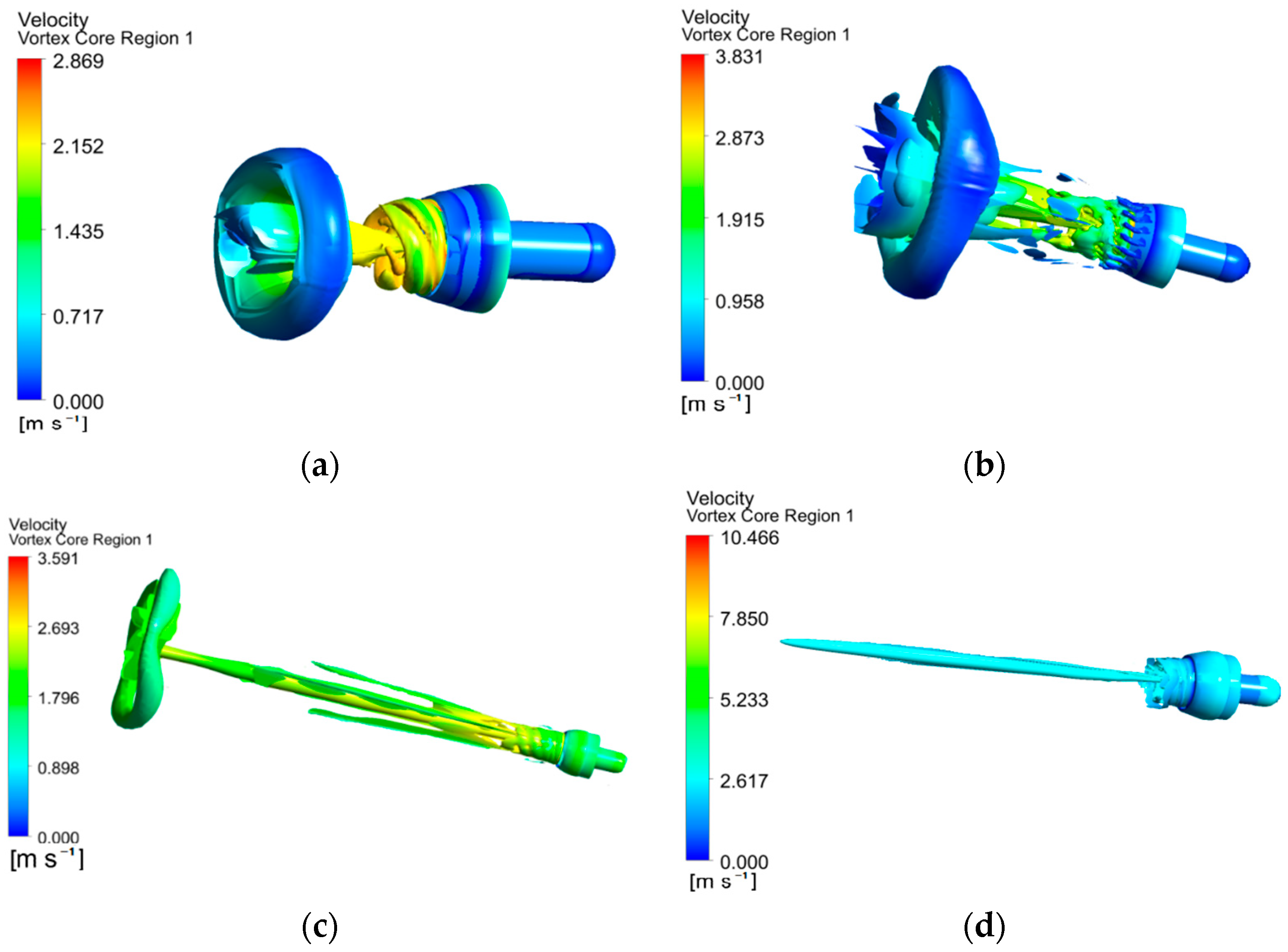
The vorticity diagram based on the Q-criterion of the ducted propeller at different navigational speeds with 2000 r/min impeller rotational speed is shown in Figure 10. It can be seen that an annular vortex distribution is formed at the tail of the propeller, which is consistent with the velocity streamline diagram analyzed above. The annular vortex in the mooring state is closer to the duct nozzle, and the vortex generated at this place will be an important part of the flow induced noise source of the propeller. With the increase of navigational speed, the annular vortex gradually weakens and moves backward until it disappears.

Figure 10.
Vorticity distribution of different navigational speed with 2000 r/min impeller rotational speed. (a) 0 m/s; (b) 0.37 m/s; (c) 1.54 m/s;(d) 2.057 m/s.
Entropy production is due to the dissipation effect caused by irreversible factors in the process, and it converts the lost mechanical energy into internal energy. The energy dissipation of the ducted thruster flow field flow can be accurately evaluated by entropy production theory. The total entropy production in the computational domain can be defined as:
where is direct dissipative entropy production, is turbulent flow dissipation entropy production, and is wall entropy production, which are defined as:
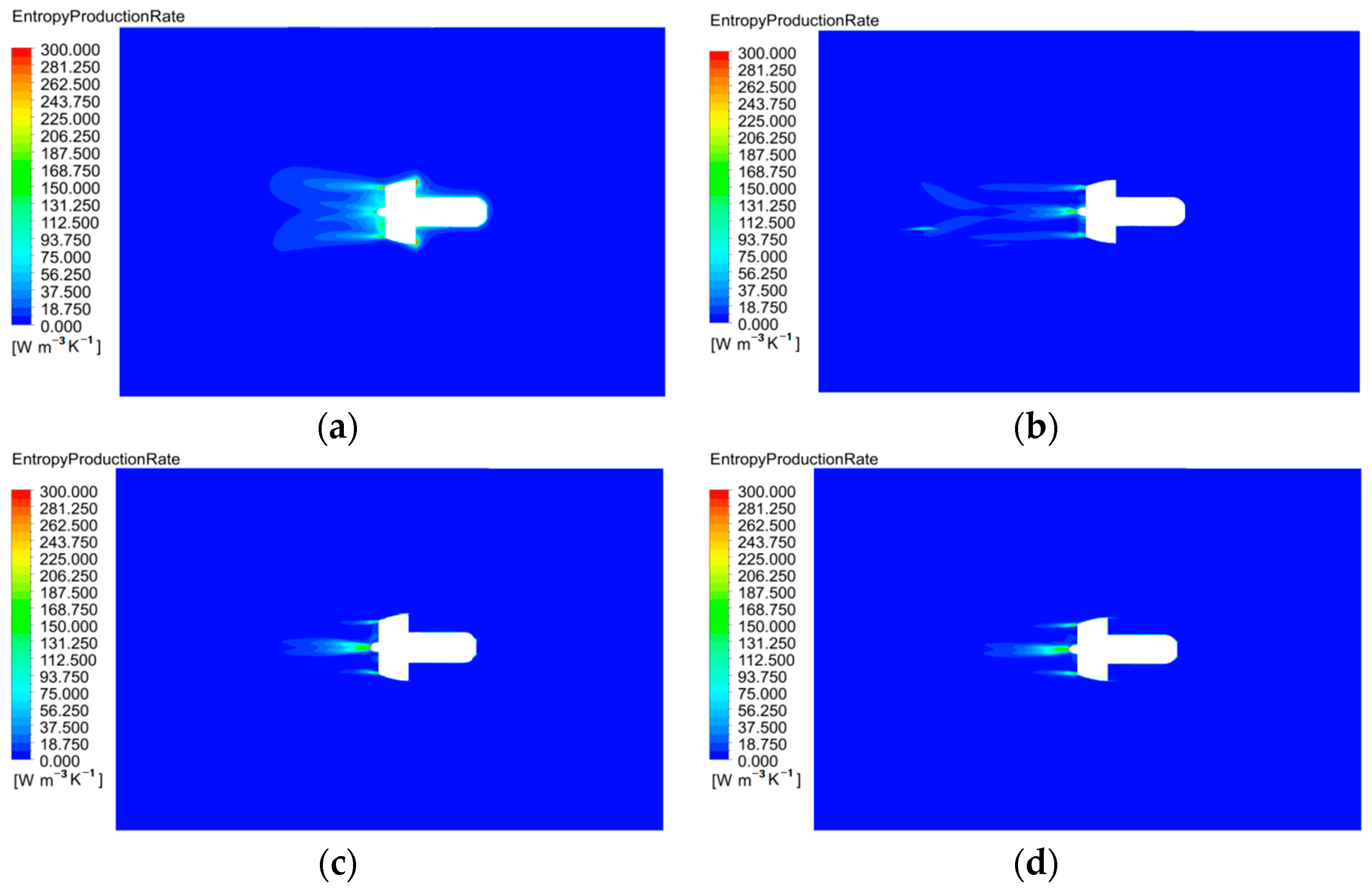
The flow field entropy cloud generation diagram of the ducted propeller under different navigational speeds when the impeller rotational speed is 2000 r/min is shown in Figure 11. It can be seen that the entropy production of the propeller is mainly concentrated at the tail of the hub and blade tip; that is, the energy loss is mainly distributed at those area, which is consistent with the vorticity distribution of the flow field analyzed above. The main energy loss area in the mooring state is closer to the nozzle, and the size of the loss area is also bigger. With the increase of navigational speed, the energy loss area of the propeller gradually expands to the rear, and the energy loss firstly decreases and then increases. The energy loss appear the smallest when the navigational speed is 1.54 m/s. This also indicates that the energy loss of the propeller in the mooring state is more serious and the noise may be stronger. On the contrary, when the speed is 1.54 m/s, the noise can be the weakest condition.
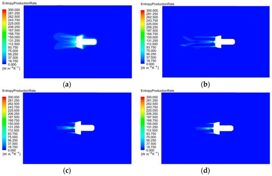
Figure 11.
Entropy distribution of different navigational speed with 2000 r/min impeller rotational speed. (a) 0 m/s; (b) 0.37 m/s; (c) 1.54 m/s; (d) 2.057 m/s.
4.3. Hydrodynamic Noise Results Analysis
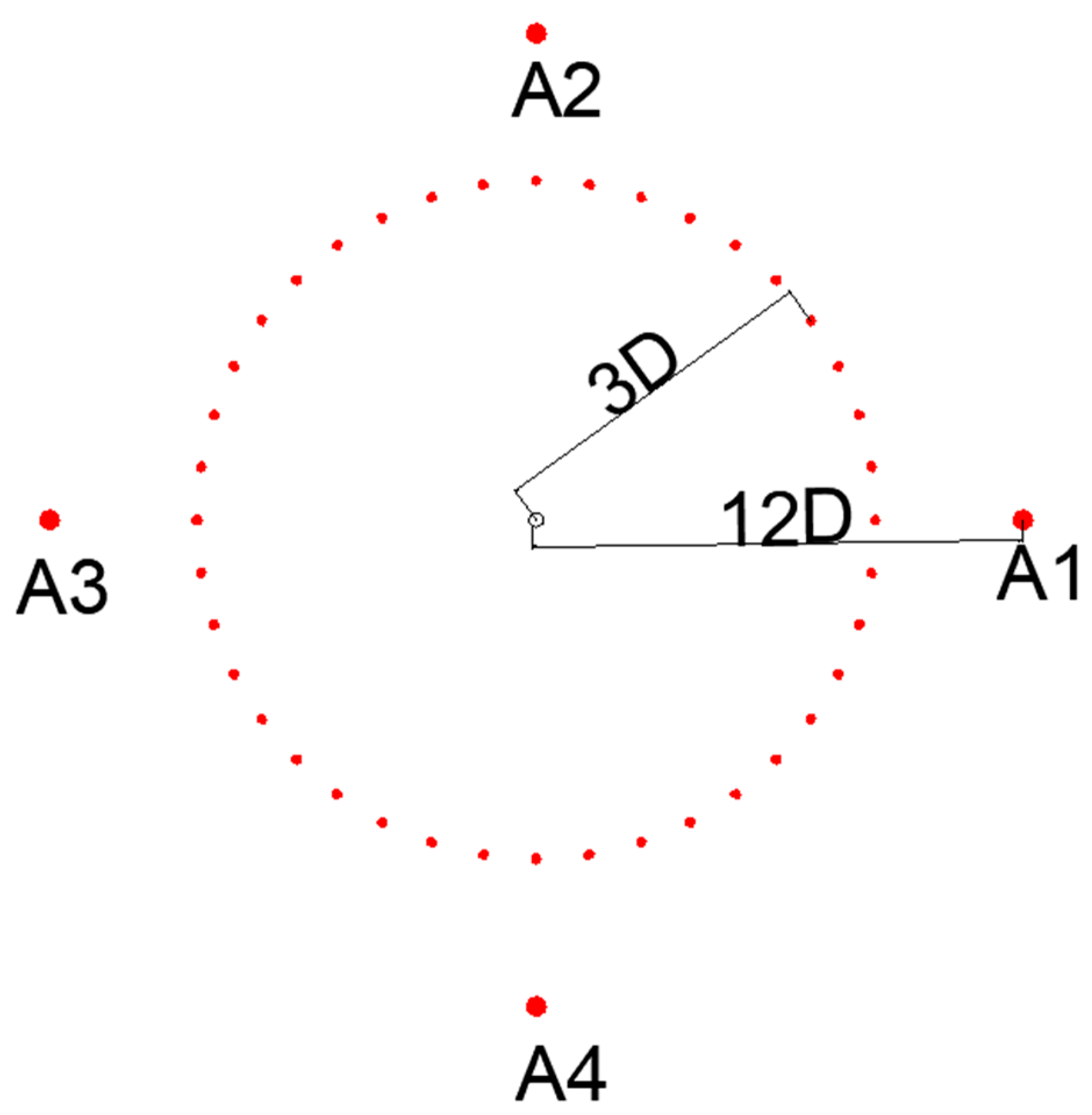
Two types of acoustic monitoring point are set as shown in Figure 12. Monitoring points (A1, A2, A3 and A4) are set in the front, rear, left and right directions away from the propeller impeller with 12D distance. In addition, forty monitoring points (B1, B2, … B40) are evenly set on the circle with radius as 3D, and the axis of the propeller impeller is the center of the circle.
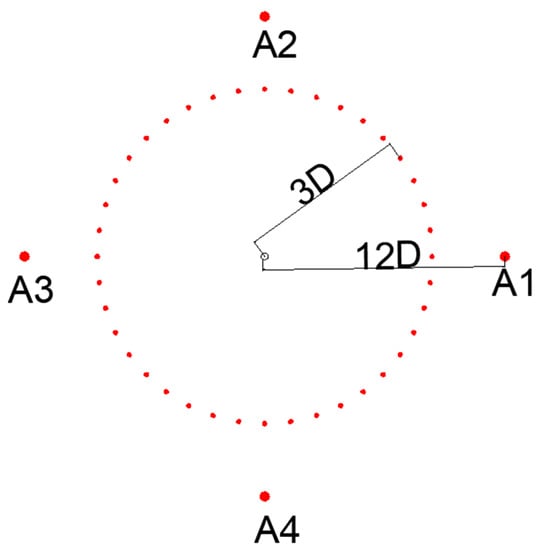
Figure 12.
Acoustic monitoring points setting.
The definition of sound pressure level and total sound pressure level is shown in the following formula.
where is the effective value of sound pressure to be measured in each frequency band, is the reference sound pressure valued by 10−6 Pa at underwater condition, is the maximum frequency and is the minimum frequency.
4.3.1. Sound Pressure Level Spectrum at Different Monitoring Points
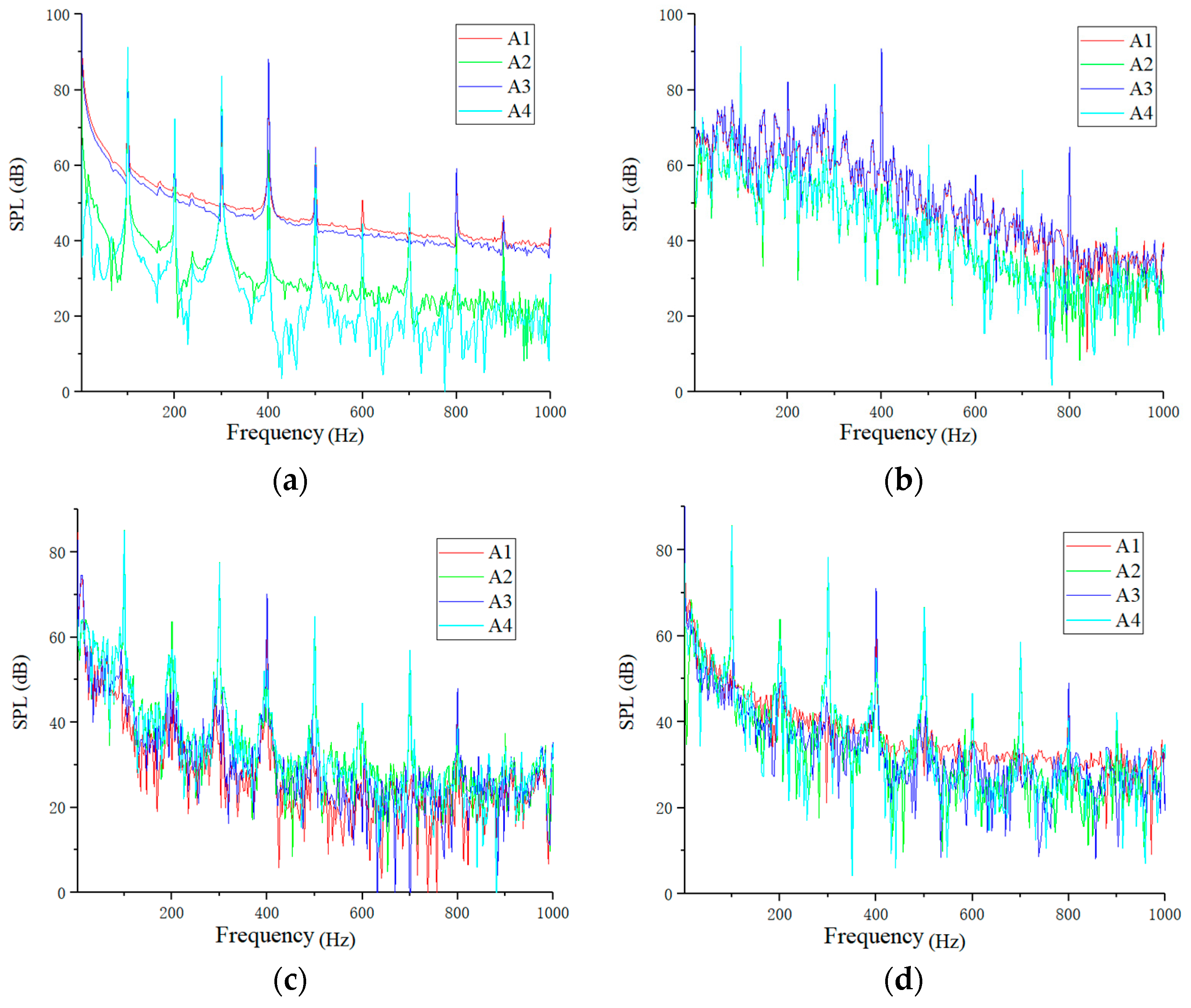
The spectrum diagram of sound pressure levels at different monitoring points of class A under the condition of impeller rotating speed of 2000 r/min and different navigational speed are shown in Figure 13. It can be seen that the sound pressure at the measuring points directly behind the propeller (A1) is the largest, followed by the measuring points directly in front (A3), and the sound pressure at the measuring points on the left (A2) and right sides (A4) are the smallest. With the increase of the navigational speed, the sound pressure level at the measuring points gradually decreases, which is consistent with the flow field analysis results above. At the same time, the sound pressure level difference between different measuring points is also decreasing with the increase of the navigational speed. The blade frequency is 100 Hz when the impeller rotational speed of the ducted propeller is 2000 r/min. It can be seen that the sound pressure level spectrum of the propeller has obvious blade passing frequency characteristics; that is, there is an obvious peak at the blade passing frequency and its multiple. However, with the increase of navigational speed, the blade passing frequency characteristics gradually weaken, showing the trend of broadband spectrum noise, and most of the noise energy is concentrated in the frequencies below five blade passing frequency. At high navigational speed, the low frequency characteristics below 100 Hz increase more and the amplitude becomes larger. This indicates that the component of turbulent noise becomes important with the increase of navigational speed.
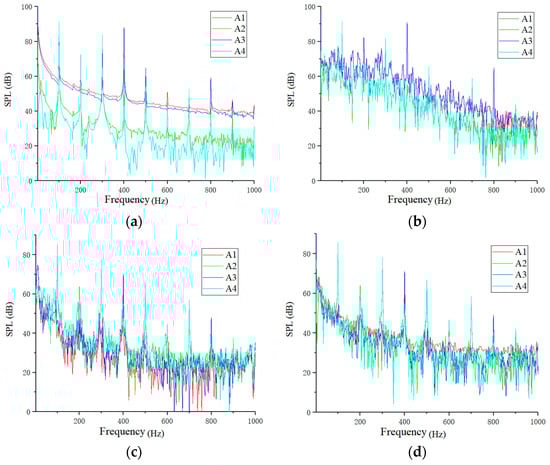
Figure 13.
The spectrum diagram of SPL of class A monitoring points at different navigational speed. (a) 0 m/s; (b) 0.37 m/s; (c) 1.54 m/s; (d) 2.057 m/s.
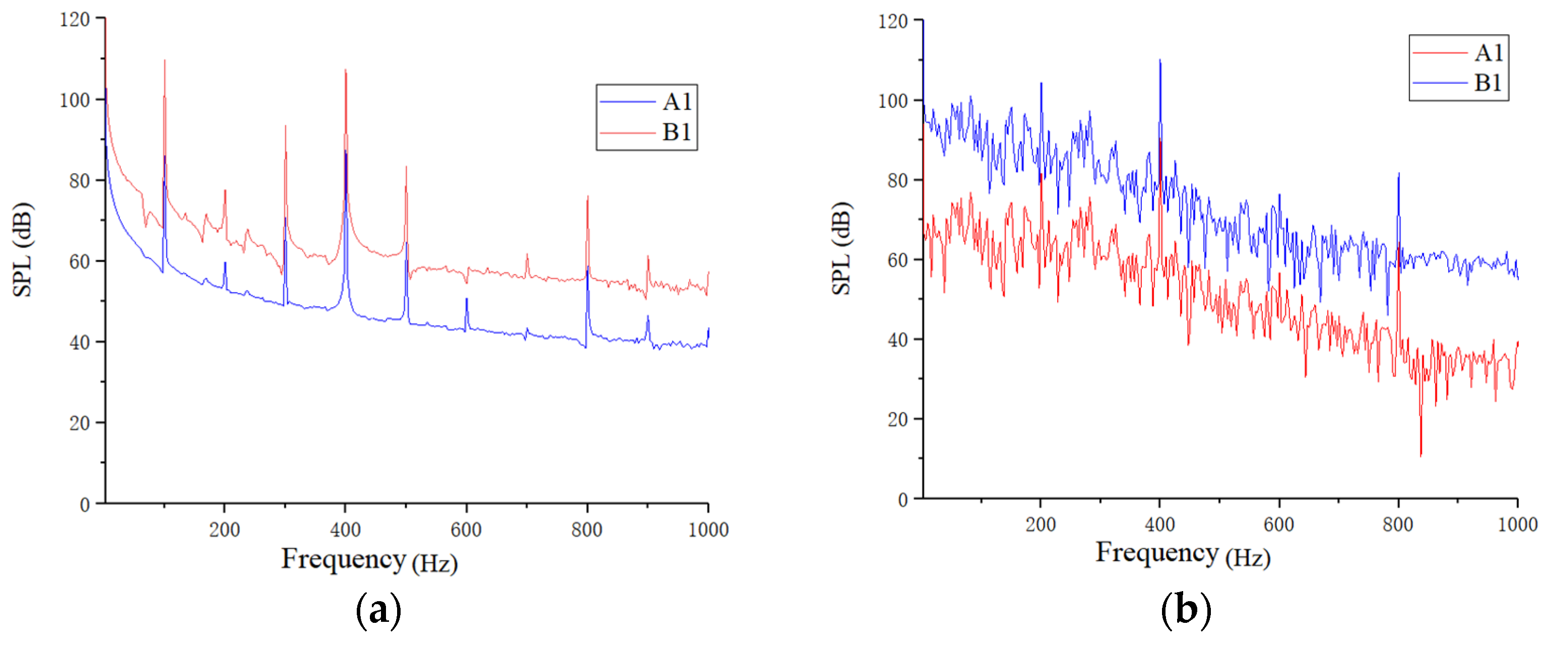
The spectrum of sound pressure levels at monitoring points A1 and B1 of the ducted propeller under the impeller rotational speed of 2000 r/min and different navigational speeds is shown in Figure 14. Monitoring point A1 and monitoring point B1 are in the same direction of the propeller, but with different distance. It can be seen that the amplitude of sound pressure level in the propeller wake area decreases with the increase of distance in all spectra. Although monitoring point B1 shows the same discrete frequency to monitoring point A1, the sound pressure level difference between measuring point A1 and measuring point B1 is less than 13 dB. In addition, the sound pressure levels of point B1 shows the same trend and frequency domain characteristics to point A1 with the increase of navigational speed. Both of the two monitoring points show that the amplitude at 4fBPF is the highest compared with the 2fBPF and 3fBPF, which might be due to the interference of the four supports in front of the impeller.

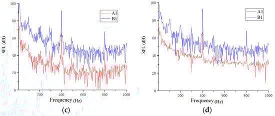
Figure 14.
The spectrum diagram of SPL of monitoring point A1 and B1 at different navigational speed. (a) 0 m/s; (b) 0.37 m/s; (c) 1.54 m/s; (d) 2.057 m/s.
4.3.2. Acoustic Directivity Analysis
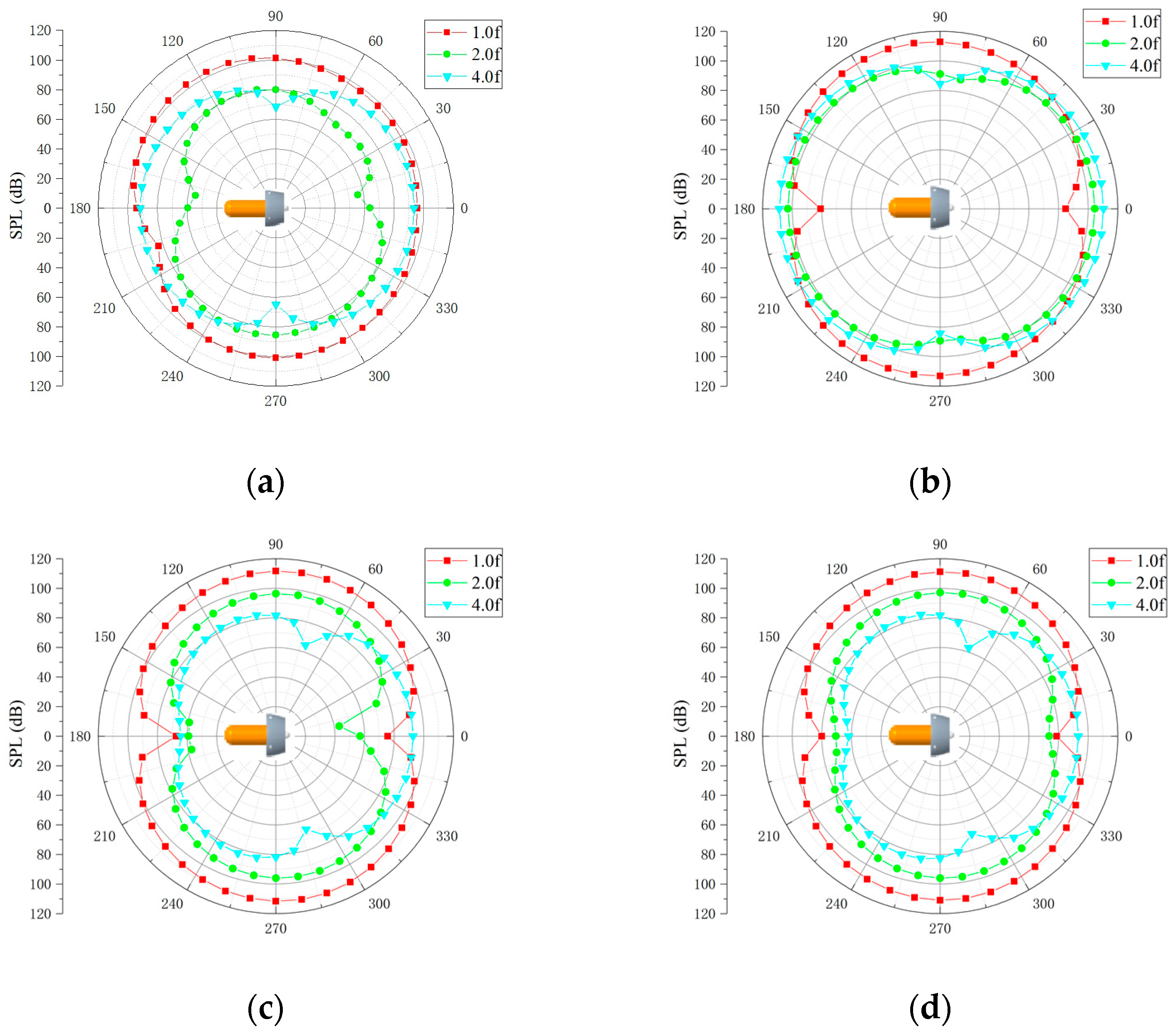
The directivity diagrams of sound pressure level at fBPF and multiple fBPF of ducted propeller under the impeller rotational speed of 2000 r/min and different navigational speeds are shown in Figure 15. It can be seen that the ducted propeller shows obvious dipole characteristics at one, two and four times of blade passing frequencies, which shows that the blade surface pressure pulsation as a dipole sound source is the main contributor to the total hydrodynamic noise. It shows “8” type at fBPF and 2 fBPF, while “∞” type at 4 fBPF. In addition, the overall acoustic directivity remains unchanged with the increase of navigational speed, but the values of each monitoring point change.
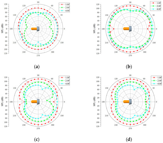
Figure 15.
Directivity diagram of sound pressure level at different navigational speeds. (a) 0 m/s; (b) 0.37 m/s; (c) 1.54 m/s; (d) 2.057 m/s.
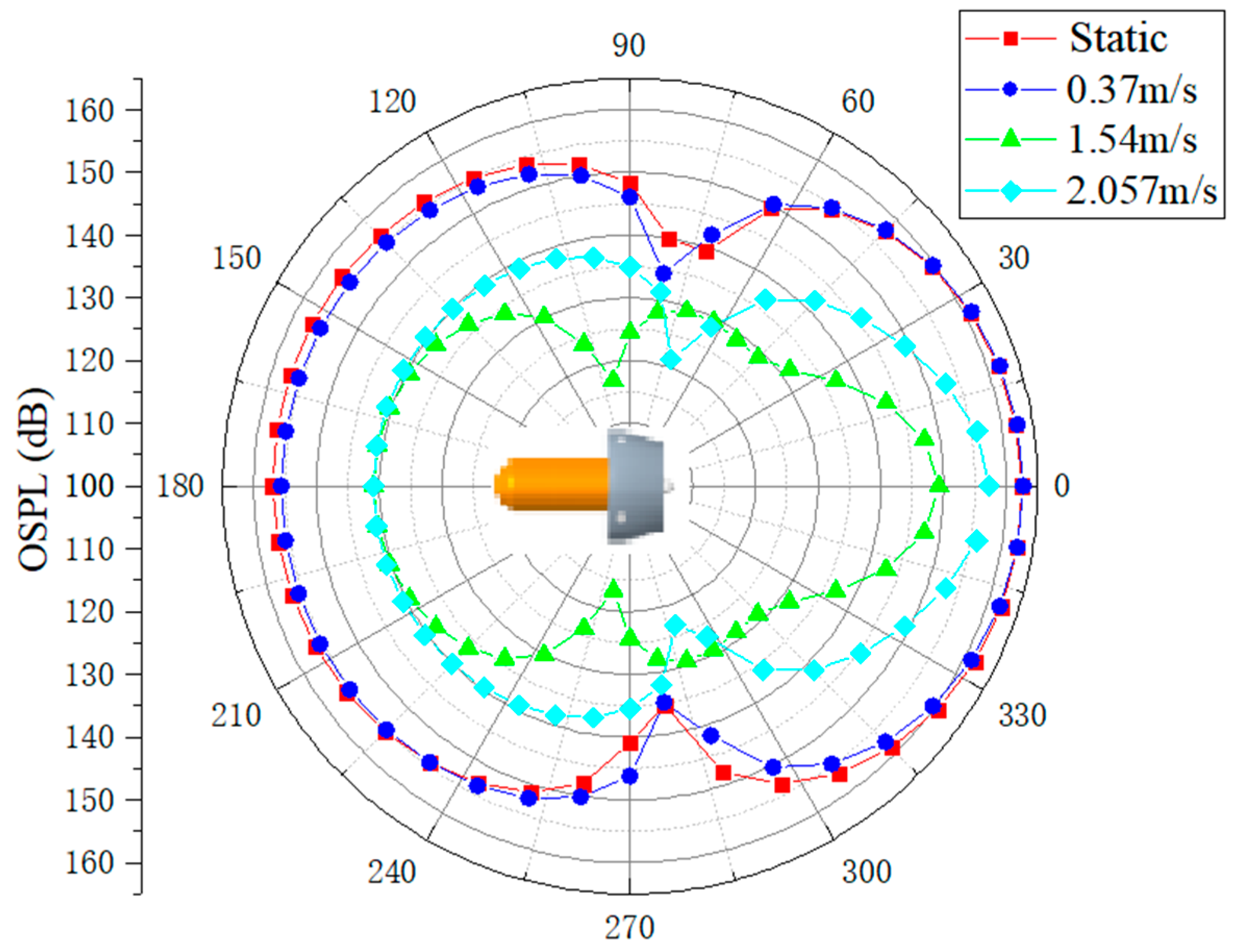
The acoustic directivity diagram of the total sound pressure level is shown in Figure 16. It presents the value of the ducted propeller at the impeller rotational speed of 2000 r/min and at different navigational speeds. It can be seen that the total sound pressure level of the propeller under all navigational speed conditions also presents a partial “∞” dipole distribution. The total sound pressure level behind the propeller is larger than that in front, and the difference between them gradually increases with the increase of navigational speed. This is because there is a strong energy exchange process and strong vortex distribution in the propeller wake area, which is an important contributor to the sound source. In addition, with the increase of navigational speed, the total sound pressure level of the propeller firstly increases and then decreases, and the sound pressure level appears the smallest when the navigational speed is 1.54 m/s, which is consistent with the results of flow field analysis; that is, when the efficiency is the highest, the noise of the propeller is the smallest.
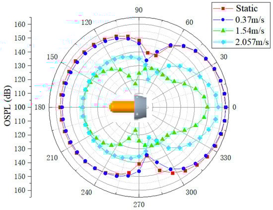
Figure 16.
Directivity diagram of total sound pressure level at different navigational speeds.
5. Conclusions
The hybrid techniques based on acoustic analogy theory are adopted in the present study to calculate the unsteady flow field and sound field characteristics of a ducted propeller. The full-scale flow filed of the propulsion system are analyzed after DES and the flow characteristic of wake vortex structure of the propeller are analyzed by entropy generation. Hydrodynamic noise of the ducted propeller flow field is calculateed by FWH equation. The frequency domain and directivity of sound pressure level at different sound field monitoring points are analyzed at four navigational speeds. The main conclusions of this paper are as follows.
- (1)
- The thrust of the studied ducted propeller at high navigational speeds is greater than that under mooring conditions. Under the fixed impeller rotational speed, the propulsion efficiency of ducted propeller increases first and then decreases with the increase of navigational speed. Numerical simulation results of the flow field are in good agreement with the experiment. The maximum errors of thrust and power are 0.5% and 0.1%, respectively, which means that the adopted DES numerical simulation method has high credibility in calculating the acoustic source.
- (2)
- There are symmetrical vortices closer to the duct outlet at the mooring state and 0.37 m/s navigational speeds; however, the pair of vortices in the wake area gradually disappear and the flow lines become more layered as the navigational speed increases, the annular vortex also gradually weakens and moves backward until it disappears. At impeller rotational speed of 2000 r/min, the best state of flow field distribution is at the navigational speed of 1.54 m/s, which is corresponding to the highest propulsion efficiency condition.
- (3)
- The propeller noise presents obvious blade passing frequency and its multiple characteristics, and most of the noise contribution is concentrated below 4fBPF. However, with the increase of speed, the blade frequency characteristics of propeller noise gradually weaken, showing the trend of continuous broadband spectrum noise. The acoustic directivity of the ducted propeller present dipole characteristic in all working conditions. At the impeller rotational speed of 2000 r/min, the sound pressure level of the propeller first decreases and then increases with the increase of the navigational speed, and the total sound pressure level of the hydrodynamic noise is the smallest at the optimal efficiency condition (the navigational speed is 1.54 m/s). At high navigational speed, the low frequency characteristics below fBPF increase more and the amplitude becomes larger. This indicates that the component of turbulent noise becomes more important with the increase of navigational speed.
Author Contributions
Conceived and designed the experiments, Q.S. and J.Y.; performed the experiments and simulation, Q.S and M.C.; analyzed the data, J.L. and Y.L.; wrote the paper, M.C.; funding acquisition, Z.J. All authors have read and agreed to the published version of the manuscript.
Funding
This research was funded by National Natural Science Foundation of China (51976079), National Key R&D Program of China (2020YFC1512400), Research Project of State Key Laboratory of Mechanical System and Vibration (MSV202201), Industry-University-Research Cooperation Project in Jiangsu Province (BY2019059).
Institutional Review Board Statement
Not applicable.
Informed Consent Statement
Not applicable.
Data Availability Statement
Not applicable.
Acknowledgments
This work were partially supported by the Research Center of Fluid Machinery Engineering and Technology and China Ship Science Research Center.
Conflicts of Interest
The authors declare no conflict of interest.
References
- Bingham, B.; Foley, B.; Singh, H.; Camilli, R.; Dellaporta, K.; Eustice, R.; Mallios, A.; Mindell, D.; Roman, C.; Sakellariou, D. Robotic tools for deep water archaeology: Surveying an ancient shipwreck with an autonomous underwater vehicle. J. Field Robot. 2010, 27, 702–717. [Google Scholar] [CrossRef] [Green Version]
- Wynn, R.B.; Huvenne, V.A.; Le Bas, T.P.; Murton, B.J.; Connelly, D.P.; Bett, B.J.; Ruhl, H.A.; Morris, K.J.; Peakall, J.; Parsons, D.R.; et al. Autonomous Underwater Vehicles (AUVs): Their past, present and future contributions to the advancement of marine geoscience. Mar. Geol. 2014, 352, 451–468. [Google Scholar] [CrossRef] [Green Version]
- Tadros, M.; Ventura, M.; Guedes Soares, C. Design of Propeller Series Optimizing Fuel Consumption and Propeller Efficiency. J. Mar. Sci. Eng. 2021, 9, 1226. [Google Scholar] [CrossRef]
- Kimmerl, J.; Mertes, P.; Abdel-Maksoud, M. Application of large eddy simulation to predict underwater noise of marine propulsors. Part 2: Noise generation. J. Mar. Sci. Eng. 2021, 9, 778. [Google Scholar] [CrossRef]
- Carlton, J. Marine Propellers and Propulsion, 2nd ed.; Butterworth-Heinemann: Oxford, UK, 2012. [Google Scholar]
- Gaafary, M.M.; El-Kilani, H.S.; Moustafa, M.M. Optimum design of B-series marine propellers. Alex. Eng. J. 2011, 50, 13–18. [Google Scholar] [CrossRef] [Green Version]
- Mirjalili, S.; Lewis, A.; Mirjalili, S.A.M. Multi-objective Optimisation of Marine Propellers. Procedia Comput. Sci. 2015, 51, 2247–2256. [Google Scholar] [CrossRef] [Green Version]
- Gaggero, S.; Tani, G.; Villa, D.; Viviani, M.; Ausonio, P.; Travi, P.; Bizzarri, G.; Serra, F. Efficient and multi-objective cavitating propeller optimization: An application to a high-speed craft. Appl. Ocean Res. 2017, 64, 31–57. [Google Scholar] [CrossRef]
- Lu, R.; Yuan, J.; Wei, G.; Zhang, Y.; Lei, X.; Si, Q. Optimization Design of Energy-Saving Mixed Flow Pump Based on MIGA-RBF Algorithm. Machines 2021, 9, 365. [Google Scholar] [CrossRef]
- Vasudev, K.L.; Sharma, R.; Bhattacharyya, S.K. Shape optimisation of an AUV with ducted propeller using GA integ-rated with CFD. Ships Offshore Struct. 2018, 13, 194–207. [Google Scholar] [CrossRef]
- Lighthill, M.J. On sound generated aerodynamically II. Turbulence as a source of sound. Proc. R. Soc. Lond. Ser. A Math. Phys. Sci. 1954, 222, 1–32. [Google Scholar]
- Oweis, G.F.; Ceccio, S.L. Instantaneous and time-averaged flow fields of multiple vortices in the tip region of a ducted propulsor. Exp. Fluid 2005, 38, 615–636. [Google Scholar] [CrossRef] [Green Version]
- Shamsi, R.; Ghassemi, H.; Molyneux, D.; Liu, P. Numerical hydrodynamic evaluation of propeller (with hub taper) and podded drive in azimuthing conditions. Ocean Eng. 2014, 76, 121–135. [Google Scholar] [CrossRef]
- Razaghian, A.H.; Ghassemi, H. Numerical analysis of the hydrodynamic characteristics of the accelerating and decelerating ducted propeller. Zesz. Nauk. Akad. Mor. Szczec. 2016, 47, 42–53. [Google Scholar]
- Chamanara, M.; Ghassemi, H. Hydrodynamic characteristics of the kort-nozzle propeller by different turbulence models. Am. J. Mech. Eng. 2016, 4, 169–172. [Google Scholar]
- Qiu, C.C.; Pan, G.; Huang, Q.G.; Shi, Y. Numerical analysis of unsteady hydrodynamic performance of pump-jet propulsor in oblique flow. Int. J. Nav. Archit. Ocean. Eng. 2019, 12, 102–115. [Google Scholar] [CrossRef]
- Kumar, P.; Mahesh, K. Large eddy simulation of propeller wake instabilities. J. Fluid Mech. 2017, 814, 361–396. [Google Scholar] [CrossRef]
- Zhang, Q.; Jaiman Rajeev, K. Numerical analysis on the wake dynamics of a ducted propeller. Ocean. Eng. 2019, 171, 202–224. [Google Scholar] [CrossRef]
- Ebrahimi, A.; Seif, M.S.; Nouri-Borujerdi, A. Hydro-acoustic and hydrodynamic optimization of a marine propeller using genetic algorithm, boundary element method, and FW-H equations. J. Mar. Sci. Eng. 2019, 7, 321. [Google Scholar] [CrossRef] [Green Version]
- Wang, Y.J.; Göttsche, U.; Abdel-Maksoud, M. Sound field properties of non-cavitating marine propellers. J. Mar. Sci. Eng. 2020, 8, 885. [Google Scholar] [CrossRef]
- Yang, Q.; Wang, Y.; Zhang, Z. Numerical prediction of the fluctuating noise source of waterjet in full scale. J. Mar. Sci. Technol. 2014, 19, 510–527. [Google Scholar] [CrossRef]
- Menter, F.R. Zonal two equation k-ω turbulence model for aerodynamic flows. In Proceedings of the 24th Fluid Dynamics Conference, AIAA, Orlando, FL, USA, 6–9 July 1993; pp. 93–2906. [Google Scholar]
- Si, Q.R.; Wang, B.B.; Yuan, J.P.; Huang, K.L.; Lin, G. Numerical and experimental investigation on radiated noise characteristics of the multistage centrifugal pump. Processes 2019, 7, 793. [Google Scholar] [CrossRef] [Green Version]
- Williams, J.F.; Hawkings, D.L. Sound generation by turbulence and surfaces in arbitrary motion. Philos. Trans. R. Soc. Lond. A 1969, 264, 321–342. [Google Scholar]
- ANSYS Help 17.2; ANSYS: Canonsburg, PA, USA, 2016.


Publisher’s Note: MDPI stays neutral with regard to jurisdictional claims in published maps and institutional affiliations. |
© 2022 by the authors. Licensee MDPI, Basel, Switzerland. This article is an open access article distributed under the terms and conditions of the Creative Commons Attribution (CC BY) license (https://creativecommons.org/licenses/by/4.0/).