A Mathematical Modeling Method for an Analytical Solution of Ship Hydrodynamic Pressure Fields in Complex Restricted Waters

Abstract

A ship advancing in restricted waters may cause a change in the surrounding velocity field, which in turn results in the hydrodynamic pressure field according to the variations in the ship speed. Accurate prediction of ship hydrodynamic pressure fields in restricted waters is therefore essential and important in the military and engineering fields. Based on the potential flow theory and the thin-ship assumption, dividing complex restricted waters with varying depths into the inner and outer domains with constant depths, a mathematical modeling method is developed and carried out for analyzing and solving the partial differential equations consisting of the governing equation with a dispersion effect, initial and boundary conditions, then the analytical solution of hydrodynamic pressure field caused by a ship advancing in complex restricted waters is obtained. The continuity of the analytical solution is confirmed and the correctness of the analytical solution is validated by simplifying to a simple water and comparing with available data. Moreover, the mathematical modeling method can be extended to study the hydrodynamic problems of ships in more complex waters.

1. Introduction

There are numerous restricted waters in the world, such as narrow waters and shallow waters. For example, for the inland waters in China, 77.7% of the water depths are less than 50 m; restricted waters account for a large proportion [1], thus, studies related to restricted waters are of practical interest. A ship advancing in restricted waters may cause a change in the surrounding velocity field, which in turn results in the hydrodynamic pressure field according to the variations in the ship speed. As we know, as the restricted waters become shallower or narrower, that is, the smaller the ship-bottom and ship-shore distances, the more the complex the variations in the hydrodynamic pressure are, which may pose greater risks to ship safety [2]. Therefore, research on ships advancing in restricted waters is of great significance, both in the military and engineering fields. For example, in the military field, since the pressure fluctuations caused by warships advancing in restricted waters are detectable, they are more easily to detected by military weapons, such as hydraulic mines, which pose a threat to the warship [3].

For a ship advancing through restricted waters, there are interactions of the ship with the surrounding boundaries to consider. In this paper, depending on whether the water depth varies along the water width, restricted waters can be divided into simple restricted waters, such as rectangular channels with no variation in the water depth, and complex restricted waters, such as dredged channels with variation in the water depth. Based on the potential flow theory and the thin-ship assumption, calculations and experiments on its wave or bottom hydrodynamic pressure were carried out by Tuck [4,5,6], confirming that the thin-ship assumption in restricted waters was reasonable. By using different numerical methods, the behavior and performance of ships advancing through restricted waters were studied by Terziev and Tafuni [7,8,9], and their research confirmed that the change in the sinkage or trim of ship had little effect on the far fields, such as the velocity or pressure fields on the sea bottom. However, the above-mentioned studies mainly focused on ship hydrodynamics in simple restricted waters and did not examine ship hydrodynamics in complex restricted waters. Some researchers, such as Gourlay [10,11,12,13], extended from simple restricted waters to complex restricted waters, and the sinkage and trim of a ship advancing through the complex restricted waters were calculated based on the potential flow theory and the thin-ship assumption. Gourlay’s results were in good agreement with the experiments, but such a technique did not take into account the dispersion effect when a ship advanced at high speed. Therefore, in order to solve ship hydrodynamic problems in complex restricted waters, we studied a mathematical modeling method for an analytical solution taking into account the dispersion effect, on the basis of our previous research [14,15,16,17,18]. The purpose is to gain further understanding of an analytical solution that can be directly expressed mathematically for ship hydrodynamic pressure fields in complex restricted waters. However, since there are some mathematical difficulties in the treatment of the hull boundary, the method of approximating the ship shape to a mathematical ship shape and the thin-ship assumption are used.

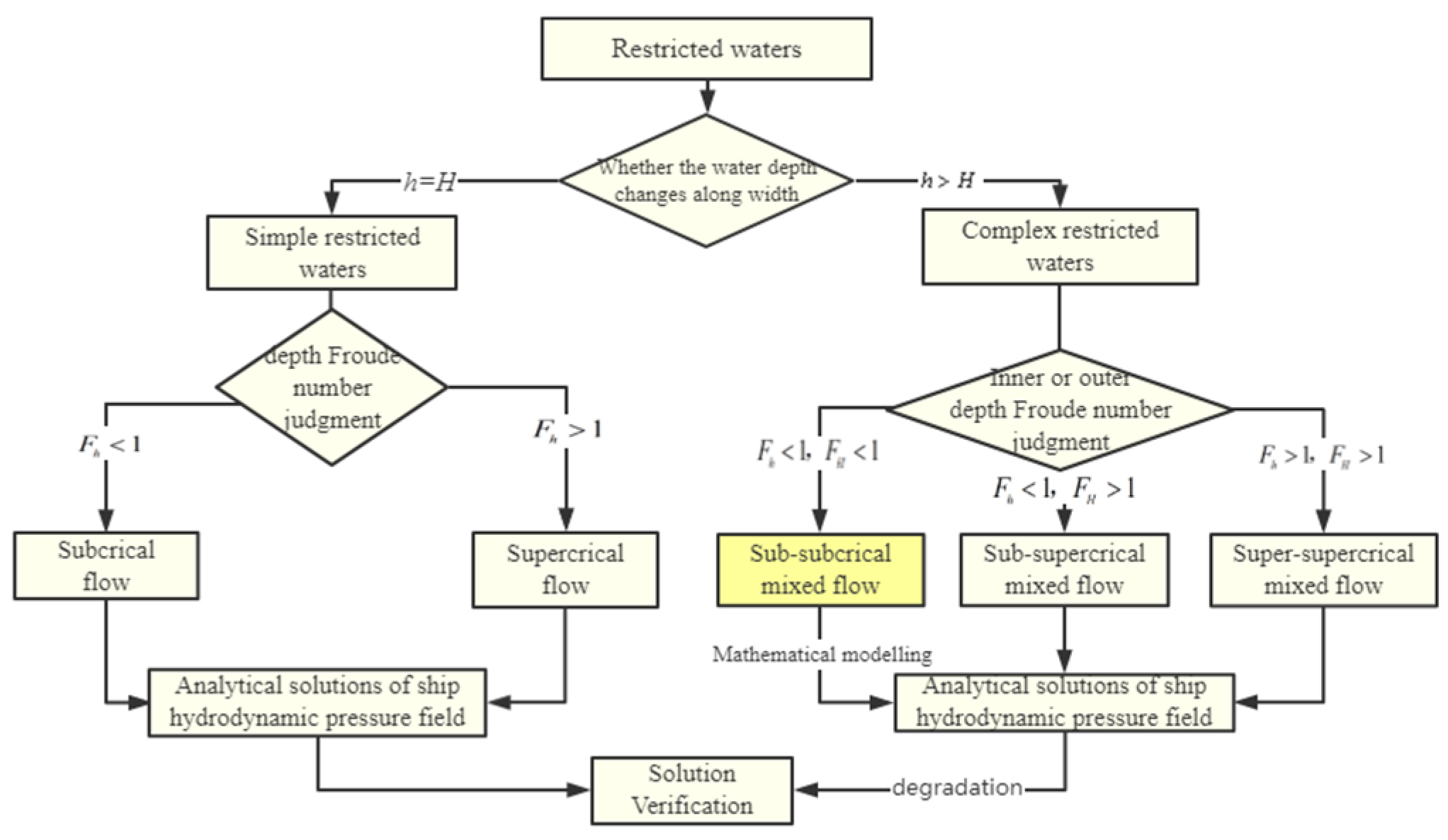
2. Mathematical Modeling

Supposing the flow field is ideal, incompressible, and non-rotational, for a ship with length L advancing at a constant speed V along the center-line of a complex restricted water, such as a dredged channel or a trapezoidal channel, a moving coordinate system with velocity V is used, where the origin O is at the center of the hull waterline, the z-axis along the water depth, positive upward, and the x-axis along the ship length, positive forward, as shown in Figure 1. The sketches for mixed flow related to the mathematical modeling method are shown in Figure 2 and Figure 3.

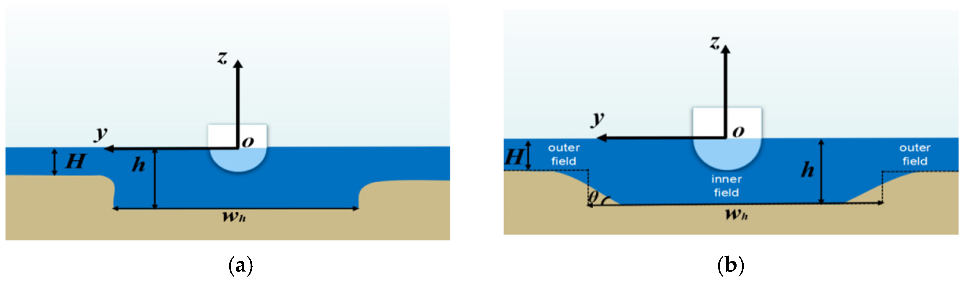
2.1. Simplification of Complex Restricted Waters

Firstly, since there is a variation in depth along the y-axis, a reasonable simplification is the first step, that is, the division of complex restricted waters with varying depths into several domains with constant depths. For a ship advancing in a dredged channel, it can be divided into two domains: an inner domain and an outer domain. For a ship advancing in a trapezoidal channel, if h/H or θ is small, the channel with slope boundaries can be simplified to the channel with stepped boundaries by transformation, and then can also be divided into two domains: an inner domain with water depth h and an outer domain with water depth H. Then, after this simplification, the study of the trapezoidal channel can be the same as that of dredged channels.

Then, supposing the inner and outer Froude numbers for depth are defined as $F_h=V/\sqrt{gh}$ and $F_H=V/\sqrt{gH}$, respectively, where h or H is the water depth in the inner or outer domain, respectively (h > H), and g is the gravitational acceleration. As is known, when$F_h$or$F_H$ <1, it is subcritical, or conversely, it is supercritical. Therefore, there are three main types of mixed flow in the complex restricted waters, because of the different$F_h$ or $F_H$, as shown in Figure 2. For example, a sub-subcritical mixed flow means that it is subcritical speed in the inner domain and subcritical speed in the outer domain, while a sub-supercritical mixed flow means that it is subcritical speed in the inner domain but supercritical speed in the outer domain, and so on.

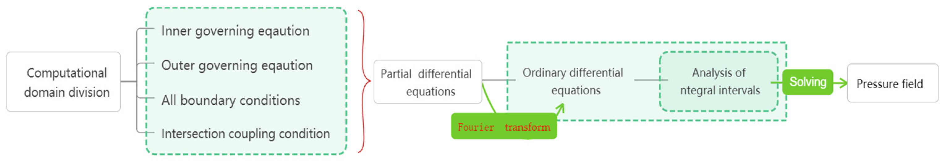
2.2. Construction of Governing Equations and Boundary Conditions

As shown in Figure 1, based on the potential flow theory, we take the shallow dredged channel as an example to develop a mathematical modeling method for the analytical solution of ship hydrodynamic pressure fields in complex restricted waters. Firstly, considering a ship moving with speed V, then the KP governing equation can be derived from the Laplace equation, the free surface and bottom conditions [18,19]:

$${\phi }_{xx}+{\phi }_{yy}+{\phi }_{zz}=0\mathrm{as}-h<z<\zeta$$

(1)

$${\zeta }_t+({\phi }_x-V){\zeta }_x+{\phi }_y{\zeta }_y-{\phi }_z=0\mathrm{on}z=\zeta$$

(2)

$${\phi }_t-V{\phi }_x+\frac{1}{2}({\phi }_x^2+{\phi }_y^2+{\phi }_z^2)+g\zeta =0\mathrm{on}z=\zeta$$

(3)

$${\phi }_z=0\mathrm{on}z=-h$$

(4)

where $\phi$ is the disturbance velocity potential, $\zeta$ is the wave height on the free surface.

Considering the characteristics of shallow water, two small parameters are defined:

$$\epsilon =A/h,\mu =h/L$$

(5)

where $\epsilon$ and $\mu$ represent the nonlinear and dispersive characteristics, respectively; A is the wave amplitude.

In order to derive a governing equation that satisfies Equations (1)–(4), the dimensionless analysis is used as:

$$(x^{*},y^{*})=(x,y)/L{z}^{*}=z/h{\zeta }^{*}=\zeta /A{\phi }^{*}=\phi /(\epsilon \sqrt{gh}L)F_h=V/\sqrt{gh}$$

(6)

where the parameters with “*” mean dimensionless parameters, while those without “*” mean dimensional ones.

For shallow water, considering Equations (1) and (4), ${\phi }^{*}$ can be expressed in terms of ${\phi }_o{}^{*}$, which is the velocity potential on the bottom, and ${\varphi }^{*}$ can be further obtained, which is the velocity potential averaged along the water depth, that is:

$${\varphi }^{*}=\frac{1}{\epsilon {\zeta }^{*}+1}{\displaystyle \underset{-1}{\overset{\epsilon {\zeta }^{*}}{\int }}{\phi }^{*}}\mathrm{d}{z}^{*}$$

(7)

where ${\phi }^{*}={\phi }_o{}^{*}-\frac{1}{2}{\mu }^2{(z^{*}+1)}^2{\nabla }^2{\phi }_o{}^{*}+\frac{1}{4!}{\mu }^4{(z^{*}+1)}^4{\nabla }^4{\phi }_o{}^{*}+\cdot \cdot \cdot$.

Equations (1)–(4) are transformed into the non-dimensional forms by using the above dimensionless analysis, and $\zeta$ can be eliminated by combining Equation (2) with Equation (3). Finally, the shallow-water governing equation can be given in the terms of the averaged velocity potential ${\varphi }^{*}$, which satisfies the Laplace equation, free surface, and bottom boundary conditions,

$$\begin{array}{l}{\nabla }^2{\varphi }^{*}-F_h^2{\varphi }^{*}{}_{x^{*}{x}^{*}}+2F_h{\varphi }^{*}{}_{x^{*}{t}^{*}}-{\varphi }^{*}{}_{t^{*}{t}^{*}}-\epsilon \left[\frac{1}{2}\right(\nabla {\varphi }^{*}·\nabla {\varphi }^{*}{)}_{t^{*}}-\frac{F_h}{2}(\nabla {\varphi }^{*}·\nabla {\varphi }^{*}{)}_{x^{*}}\\ -F_h\nabla ({\varphi }^{*}{}_{x^{*}}\nabla {\varphi }^{*})+\nabla ({\varphi }^{*}{}_{t^{*}}\nabla {\varphi }^{*}\left)\right]-\frac{1}{3}{\mu }^2{\nabla }^2(2F_h{\varphi }^{*}{}_{x^{*}{t}^{*}}-{\varphi }^{*}{}_{t^{*}{t}^{*}}-F_h^2{\varphi }^{*}{}_{x^{*}{x}^{*}})=0\end{array}$$

(8)

Further assuming the main direction of wave propagation is along the x-axis, and transforming into the dimensional form, then Equation (8) can be simplified to [13]:

$$\frac{2F_h^{}}{gh}{\varphi }_{xt}+(1-F_h^2){\varphi }_{xx}+{\varphi }_{yy}+\frac{3F_h^{}}{gh}{\varphi }_x{\varphi }_{xx}+\frac{F_h^2{h}_{}^2}{3}{\varphi }_{xxxx}=0$$

(9)

Ignoring the unsteady and nonlinear effects, and considering the dispersive effect of Equation (9), the flow in the inner and outer domains would satisfy the following governing equations:

$$(1-F_h^2){\varphi }_{xx}+{\varphi }_{yy}+\frac{F_h^2{h}_{}^2}{3}{\varphi }_{xxxx}=0\mathrm{as}\left|y\right|\le w_1$$

(10)

$$(1-F_H^2){\Phi }_{xx}+{\Phi }_{yy}+\frac{F_H^2{H}_{}^2}{3}{\Phi }_{xxxx}=0\mathrm{as}\left|y\right|\ge w_1$$

(11)

where $w_1=0.5w_h$ is the half-width of the inner domain; $\varphi$ and $\Phi$ are the inner and outer velocity potential averaged along the water depth, respectively.

Furthermore, the hull boundary condition based on the thin-ship assumption is,

$${{\varphi }_y|}_{y\to 0^{\pm }}\approx \mp \frac{V}{2h}\frac{\partial S\left(x\right)}{\partial x}\mathrm{as}\left|x\right|\le 0.5L$$

(12)

where S(x) is the underwater cross-sectional area of the hull. For a Wigley mathematical ship, there is $S\left(x\right)\approx 2Bd/3\left[1-{\left(x/0.5L\right)}^2\right]$, where B, d are the ship breadth, draft, respectively.

As z = −h, the inner and outer bottom conditions are ${\varphi }_z=0$ and ${\Phi }_z=0$, respectively. Meanwhile, the initial condition is ${\varphi |}_{t=0}=0$, because the two domains are both subcritical, the upstream and downstream infinity meet the disturbance attenuation conditions, that is, as $x\to \pm \infty$, $\varphi ,\mathit{\Phi }\to 0$.

If a ship is advancing in a stepped channel, additional sidewall conditions are required in the outer domain, i.e.,

$${{\Phi }_y|}_{y\to \pm 0.5w}=0$$

(13)

For a complex restricted water, it is also necessary to satisfy the coupling condition at the intersection of the inner and outer domains, i.e.,

$$\varphi (x,w_1-0)=\mathit{\Phi }(x,w_1+0)\mathrm{and}h{\varphi }_y(x,w_1-0)=H{\mathit{\Phi }}_y(x,w_1+0)$$

(14)

Finally, Equations (10)–(14) of the inner and outer domains together constitute the theoretical model for mixed flow in complex restricted waters.

2.3. Fourier Transform of Governing Equations and Boundary Conditions

Taking the example of a sub-subcritical mixed flow in the dredged channel, the Fourier transform is used to transform the above governing equations and boundary conditions, and the Fourier transform of other mixed flows is similar. Since the flow field is symmetrical, only the half domain is discussed, and the corresponding Fourier transform pair of the inner or outer domains is taken as:

$$\tilde{\varphi }(k,y)={\displaystyle \underset{-\infty }{\overset{\infty }{\int }}\varphi (x,y)e^{ikx}\mathrm{d}x} \tilde{\Phi }(k,y)={\displaystyle \underset{-\infty }{\overset{\infty }{\int }}\mathit{\Phi }(x,y)e^{ikx}\mathrm{d}x}$$

(15)

$$\varphi (x,y)=\frac{1}{2\pi }{\displaystyle \underset{-\infty }{\overset{\infty }{\int }}\tilde{\varphi }(k,y)e^{-ikx}\mathrm{d}k} \mathit{\Phi }(x,y)=\frac{1}{2\pi }{\displaystyle \underset{-\infty }{\overset{\infty }{\int }}\tilde{\Phi }(k,y)e^{-ikx}\mathrm{d}k}$$

(16)

2.3.1. Inner Domain

In the inner domain, using the upstream and downstream conditions, the Fourier transform of Equation (10) yields:

$${\tilde{\varphi }}_{yy}(k,y)+{\sigma }_1\tilde{\varphi }(k,y)=0\mathrm{as}y\le w_1\mathrm{and}{F}_h<1$$

(17)

where ${\sigma }_1=({\gamma }_1^2{k}^2-{\beta }_1^2)k^2$, ${\gamma }_1=F_{h}h/\sqrt{3}$, and ${\beta }_1=\sqrt{1-F_h^2}$.

When k varies between $-\infty$ and $+\infty$, two cases of k > 0 and k < 0 exist for solving Equation (17) analytically, which is discussed separately below.

If ${\sigma }_1>0$, then ${\gamma }_1^2{k}^2-{\beta }_1^2>0$, there is $k>{\beta }_1^{}/{\gamma }_1$ or $k<-{\beta }_1^{}/{\gamma }_1$, thus, the general solution of Equation (17) is given as:

$$\tilde{\varphi }(k,y)=A(k)e^{iy\sqrt{{\sigma }_1}}+B(k)e^{-iy\sqrt{{\sigma }_1}}$$

(18)

where A(k) and B(k) are unknown and needed to be solved below.

Carrying out the Fourier transform on Equation (12) of the hull boundary condition,

$${\tilde{\varphi }}_y(k,0)=iVk\tilde{f}(k)$$

(19)

where $\tilde{f}(k)={\displaystyle \underset{-\infty }{\overset{\infty }{\int }}f(x)e^{ikx}\mathrm{d}}x$, $\tilde{f}(k)$ is an even function about $k$, for a Wigley ship, it is $\tilde{f}(k)=-4Bd/3h{l}^2[l\cos (kl)/k^2-\sin (kl)/k^3]$.

Combining Equations (18) and (19), we can obtain:

$$\tilde{\varphi }(k,y)=2B(k)\cos (y\sqrt{{\sigma }_1})+\frac{kV\tilde{f}(k)e^{iy\sqrt{{\sigma }_1}}}{\sqrt{{\sigma }_1}}$$

(20)

If ${\sigma }_1<0$, then ${\gamma }_1^2{k}^2-{\beta }_1^2<0$, there is $-{\beta }_1^{}/{\gamma }_1<k<{\beta }_1^{}/{\gamma }_1$, thus, the general solution of Equation (17) is given by:

$$\tilde{\varphi }(k,y)=E(k)e^{y\sqrt{\left|{\sigma }_1\right|}}+F(k)e^{-y\sqrt{\left|{\sigma }_1\right|}}$$

(21)

Similarly, combining Equations (21) and (19), we obtain:

$$\tilde{\varphi }(k,y)=2F(k)\cosh (y\sqrt{\left|{\sigma }_1\right|})+\frac{ikV\tilde{f}(k)e^{y\sqrt{\left|{\sigma }_1\right|}}}{\sqrt{\left|{\sigma }_1\right|}}$$

(22)

2.3.2. Outer Domain

In the outer domain, the Fourier transform of Equation (11) yields:

$${\tilde{\Phi }}_{yy}(k,y)+{\sigma }_2\tilde{\Phi }(k,y)=0\mathrm{as}y\ge w_1\mathrm{and}{F}_H<1$$

(23)

where ${\sigma }_2=({\gamma }_2^2{k}^2-{\beta }_2^2)k^2$, ${\gamma }_2=F_{H}H/\sqrt{3}$, and ${\beta }_2=\sqrt{1-F_H^2}$.

If ${\sigma }_2>0$, there is $k>{\beta }_2^{}/{\gamma }_2$ or $k<-{\beta }_2^{}/{\gamma }_2$, combining with the no-wave condition in front of the ship, the general solution of Equation (23) is given as:

$$\begin{array}{c}\tilde{\Phi }(k,y)=J(k)e^{-iyk\sqrt{{\gamma }_2^2{k}^2-{\beta }_2^2}}\mathrm{as}k>{\beta }_2^{}/{\gamma }_2\mathrm{or}\\ \tilde{\Phi }(k,y)=H(k)e^{-iyk\sqrt{{\gamma }_2^2{k}^2-{\beta }_2^2}}\mathrm{as}k<-{\beta }_2^{}/{\gamma }_2\end{array}$$

(24)

If ${\sigma }_2<0$, there is $-{\beta }_2^{}/{\gamma }_2<k<{\beta }_2^{}/{\gamma }_2$, combining with the upstream and downstream conditions, the general solution of Equation (23) is given as:

$$\tilde{\Phi }(k,y)=N(k)e^{y\sqrt{\left|{\sigma }_2\right|}}+M(k)e^{-y\sqrt{\left|{\sigma }_2\right|}}$$

(25)

Then, we can obtain:

$$\begin{array}{l}\tilde{\Phi }(k,y)=M(k)e^{-yk\sqrt{{\beta }_2^2-{\gamma }_2^2{k}^2}}\mathrm{as}0<k<{\beta }_2/{\gamma }_2\mathrm{or}\\ \tilde{\Phi }(k,y)=M(k)e^{yk\sqrt{{\beta }_2^2-{\gamma }_2^2{k}^2}}\mathrm{as}-{\beta }_2/{\gamma }_2<k<0\end{array}$$

(26)

The Fourier transform of Equation (14) at the intersection is:

$$\tilde{\varphi }(k,w_1-0)=\tilde{\Phi }(k,w_1+0)\mathrm{and}h{\tilde{\varphi }}_y(k,w_1-0)=H{\tilde{\Phi }}_y(k,w_1+0)$$

(27)

3. Derivation of Analytical Solution

In the mathematical modeling study of mixed flow, the analysis of integral intervals is important. For a sub-subcritical mixed flow in complex restricted waters, there are two cases: k > 0 and k < 0. Firstly, considering the case of k > 0, the inner solution needs to be solved in two intervals: $0<k<{\beta }_1/{\gamma }_1$ and $k>{\beta }_1/{\gamma }_1$; meanwhile, the outer solution needs to be solved in two intervals: $0<k<{\beta }_2/{\gamma }_2$ and $k>{\beta }_2/{\gamma }_2$. Since the inner and outer integral intervals do not overlap, we need to repartition them so that the solution can be in the same integral interval. Therefore, the problem for a mixed flow needs to be analyzed and solved for several integral intervals, according to the different mathematical characteristics.

3.1. Analytical Solution of the Velocity Field for a Sub-Subcritical Mixed Flow

With the different ship speeds and water depths, there may be both cases which need to be determined in advance, for example, if there is $V>\sqrt{ghH/(h+H)}$, then ${\beta }_1/{\gamma }_1>{\beta }_2/{\gamma }_2$, conversely, ${\beta }_1/{\gamma }_1<{\beta }_2/{\gamma }_2$.

3.1.1. Inner Domain

When ${\beta }_1/{\gamma }_1<{\beta }_2/{\gamma }_2$, if k > 0, there are $0<k<{\beta }_1/{\gamma }_1$, ${\beta }_1/{\gamma }_1<k<{\beta }_2/{\gamma }_2$ and $k>{\beta }_2/{\gamma }_2$. The inner and outer domains should be solved separately for each integral interval.

As $0<k<{\beta }_1/{\gamma }_1$, using Equations (22), (26) and (27) to obtain:

$$F(k)=\frac{-i(1+d_1)Vk\tilde{f}(k)e^{w_1{t}_1}}{2t_1[\sinh (w_1{t}_1)+d_1\cosh (w_1{t}_1)]}$$

(28)

where $t_1=k\sqrt{{\beta }_1^2-{\gamma }_1^2{k}^2}$, $d_1=H{t}_2/(h{t}_1)$.

Substituting Equation (28) into Equation (22), the inner solution is obtained as:

$$\tilde{\varphi }(k,y)=-iVk\tilde{f}(k)\frac{\cosh [(w_1-y)t_1]+d_1\sinh [(w_1-y)t_1]}{t_1[\sinh (w_1{t}_1)+d_1\cosh (w_1{t}_1)]}$$

(29)

As ${\beta }_1/{\gamma }_1<k<{\beta }_2/{\gamma }_2$, using Equations (20), (26) and (27) to obtain:

$$B(k)=\frac{(i+q_1)Vk\tilde{f}(k)e^{i{w}_1{s}_1}}{2s_1[\sin (w_1{s}_1)-q_1\cos (w_1{s}_1)]}$$

(30)

where $s_1=k\sqrt{{\gamma }_1^2{k}^2-{\beta }_1^2}$, $q_1=H{t}_2/(h{s}_1)$.

Substituting Equation (30) into Equation (20), the inner solution is obtained as:

$$\tilde{\varphi }(k,y)=iVk\tilde{f}(k)\frac{q_1\sin [(w_1-y)s_1]+\cos [(w_1-y)s_1]}{s_1[\sin (w_1{s}_1)-q_1\cos (w_1{s}_1)]}$$

(31)

As $k>{\beta }_2/{\gamma }_2$, using Equations (20), (24) and (27) to obtain:

$$B(k)=\frac{i(r_1+1)Vk\tilde{f}(k)e^{i{w}_1{s}_1}}{2s_1[\sin (w_1{s}_1)-i{r}_1\cos (w_1{s}_1)]}$$

(32)

where $r_1=H{s}_2/(h{s}_1)$, $s_2=k\sqrt{{\gamma }_2^2{k}^2-{\beta }_2^2}$.

Substituting Equation (32) into Equation (20), the inner solution is obtained as:

$$\tilde{\varphi }(k,y)=iVk\tilde{f}(k)\frac{\cos [(w_1-y)s_1]+i{r}_1\sin [(w_1-y)s_1]}{s_1[\sin (w_1{s}_1)-i{r}_1\cos (w_1{s}_1)]}$$

(33)

Similarly, considering the case of k < 0, it can be seen that $\tilde{\varphi }(k,y)$ for $-{\beta }_1^{}/{\gamma }_1<k<0$, $-{\beta }_2/{\gamma }_2<k<-{\beta }_1/{\gamma }_1$, and $k<-{\beta }_2/{\gamma }_2$ in the inner domain have exactly the same form as Equations (29), (31) and (33), respectively.

3.1.2. Outer Domain

The analytical method used in the subcritical inner domain is similar to that in the subcritical outer domain; there are also two cases: k > 0 and k < 0, and if k > 0, $0<k<{\beta }_1/{\gamma }_1$, ${\beta }_1/{\gamma }_1<k<{\beta }_2/{\gamma }_2$ and $k>{\beta }_2/{\gamma }_2$ exist.

As $0<k<{\beta }_1/{\gamma }_1$, using Equations (22) and (26)–(28) to obtain:

$$M(k)=-\frac{iVk\tilde{f}(k)e^{w_1{t}_2}}{t_1[\sinh (w_1{t}_1)+d_1\cosh (w_1{t}_1)]}$$

(34)

Substituting Equation (34) into Equation (26), the outer solution is obtained as:

$$\tilde{\Phi }(k,y)=-\frac{iVk\tilde{f}(k)e^{(w_1-y)t_2}}{t_1[\sinh (w_1{t}_1)+d_1\cosh (w_1{t}_1)]}$$

(35)

As ${\beta }_1/{\gamma }_1<k<{\beta }_2/{\gamma }_2$, using Equations (20), (26), (27), and (30) to obtain:

$$M(k)=\frac{iVk\tilde{f}(k)e^{w_1{t}_2}}{s_1[\sin (w_1{s}_1)-q_1\cos (w_1{s}_1)]}$$

(36)

Substituting Equation (36) into Equation (26), the outer solution is obtained as:

$$\tilde{\Phi }(k,y)=\frac{iVk\tilde{f}(k)e^{(w_1-y)t_2}}{s_1[\sin (w_1{s}_1)-q_1\cos (w_1{s}_1)]}$$

(37)

As $k>{\beta }_2/{\gamma }_2$, using Equations (20), (24), (27), and (32) to obtain:

$$J(k)=\frac{iVk\tilde{f}(k)e^{i{w}_1{s}_2}}{s_1[\sin (w_1{s}_1)-i{r}_1\cos (w_1{s}_1)]}$$

(38)

Substituting Equation (38) into Equation (24), the outer solution is obtained as:

$$\tilde{\Phi }(k,y)=\frac{iVk\tilde{f}(k)e^{i(w_1-y)s_2}}{s_1[\sin (w_1{s}_1)-i{r}_1\cos (w_1{s}_1)]}$$

(39)

Similarly, considering the case of $k<0$, it can be proven that $\tilde{\varphi }(k,y)$ for $-{\beta }_1^{}/{\gamma }_1<k<0$, $-{\beta }_2/{\gamma }_2<k<-{\beta }_1/{\gamma }_1$, and $k<-{\beta }_2/{\gamma }_2$ in the outer domain have exactly the same form as Equations (35), (37), and (39), respectively.

Finally, through the Fourier transform, the analytical solution of the inner and outer velocity field for a sub-subcritical mixed flow is obtained as:

$$\begin{array}{l}\varphi (x,y)=\frac{1}{\pi }{\displaystyle \underset{0}{\overset{\infty }{\int }}\tilde{\varphi }(k,y)e^{-ikx}\mathrm{d}k}\mathrm{as}y\le w_1\mathrm{and}{F}_h<1\\ \mathit{\Phi }(x,y)=\frac{1}{\pi }{\displaystyle \underset{0}{\overset{\infty }{\int }}\tilde{\Phi }(k,y)e^{-ikx}\mathrm{d}k}\mathrm{as}y\ge w_1\mathrm{and}{F}_H<1\end{array}$$

(40)

• where if $0<k<{\beta }_1/{\gamma }_1$, $\tilde{\varphi }(k,y)=-iVk\tilde{f}(k)\frac{\cosh [(w_1-y)t_1]+d_1\sinh [(w_1-y)t_1]}{t_1[\sinh (w_1{t}_1)+d_1\cosh (w_1{t}_1)]}$,
• $\tilde{\Phi }(k,y)=-\frac{iVk\tilde{f}(k)e^{(w_1-y)t_2}}{t_1[\sinh (w_1{t}_1)+d_1\cosh (w_1{t}_1)]}$; if ${\beta }_1/{\gamma }_1<k<{\beta }_2/{\gamma }_2$, $\tilde{\Phi }(k,y)=\frac{iVk\tilde{f}(k)e^{(w_1-y)t_2}}{s_1[\sin (w_1{s}_1)-q_1\cos (w_1{s}_1)]}$,
• $\tilde{\varphi }(k,y)=iVk\tilde{f}(k)\frac{q_1\sin [(w_1-y)s_1]+\cos [(w_1-y)s_1]}{s_1[\sin (w_1{s}_1)-q_1\cos (w_1{s}_1)]}$; if $k>{\beta }_2/{\gamma }_2$, $\tilde{\Phi }(k,y)=\frac{iVk\tilde{f}(k)e^{i(w_1-y)s_2}}{s_1[\sin (w_1{s}_1)-i{r}_1\cos (w_1{s}_1)]}$,
• $\tilde{\varphi }(k,y)=iVk\tilde{f}(k)\frac{\cos [(w_1-y)s_1]+i{r}_1\sin [(w_1-y)s_1]}{s_1[\sin (w_1{s}_1)-i{r}_1\cos (w_1{s}_1)]}$.

3.2. Analytical Solution of the Pressure Field for a Sub-Subcritical Mixed Flow

The velocity field was solved analytically first, and then the pressure field was also obtained. The disturbance pressure coefficient is defined as $C_p=\frac{\mathsf{\Delta }p}{0.5\rho V^2}$, where $\mathsf{\Delta }p=\rho V{\varphi }_x(x,y)$, $\mathsf{\Delta }p=\rho V{\Phi }_x(x,y)$ are the pressure variations in the inner or outer domains and can be linearized according to Bernoulli’s equation.

Based on Equation (40), ${\varphi }_x$ and ${\mathit{\Phi }}_x$ can be obtained. Then, the pressure field for a sub-subcritical mixed flow can be given:

$$\begin{array}{l}{C}_p(x,y)={\displaystyle \underset{0}{\overset{\infty }{\int }}g(k,y)}\mathrm{d}k\mathrm{as}y\le w_1\mathrm{and}{F}_h<1\\ C_p(x,y)={\displaystyle \underset{0}{\overset{\infty }{\int }}G(k,y})\mathrm{d}k\mathrm{as}y\ge w_1\mathrm{and}{F}_H<1\end{array}$$

(41)

• where if $0<k<{\beta }_1/{\gamma }_1$, $g(k,y)=-\frac{2k^2\tilde{f}(k)}{\pi }\frac{d_1\sinh [(w_1-y)t_1]+\cosh [(w_1-y)t_1]}{t_1[d_1\cosh (w_1{t}_1)+\sinh (w_1{t}_1)]}\cos (kx)$,
• $G(k,y)=-\frac{2k^2\tilde{f}(k)}{\pi }\frac{e^{(w_1-y)t_2}}{t_1[\sinh (w_1{t}_1)+d_1\cosh (w_1{t}_1)]}\cos (kx)$;
• if ${\beta }_1/{\gamma }_1<k<{\beta }_2/{\gamma }_2$, $g(k,y)=-\frac{2k^2\tilde{f}(k)}{\pi }\frac{q_1\sin [(w_1-y)s_1]+\cos [(w_1-y)s_1]}{s_1[q_1\cos (w_1{s}_1)-\sin (w_1{s}_1)]}\cos (kx)$,
• $G(k,y)=\frac{2k^2\tilde{f}(k)}{\pi }\frac{e^{(w_1-y)t_2}}{s_1[\sin (w_1{s}_1)-q_1\cos (w_1{s}_1)]}\cos (kx)$;
• if $k>{\beta }_2/{\gamma }_2$, $g(k,y)=-\frac{2k^2\tilde{f}(k)}{\pi }\frac{r_1^2\sin [(w_1-y)s_1]\cos (kx)\cos (w_1{s}_1)-r_1\sin (kx)\cos (y{s}_1)}{s_1[r_1^2{\cos }^2(w_1{s}_1)+{\sin }^2(w_1{s}_1)]}$
  $+\frac{2k^2\tilde{f}(k)}{\pi }\frac{\cos [(w_1-y)s_1]\cos (kx)\sin (w_1{s}_1)}{s_1[r_1^2{\cos }^2(w_1{s}_1)+{\sin }^2(w_1{s}_1)]}$,
• $G(k,y)=\frac{2k^2\tilde{f}(k)}{\pi }\frac{\cos [kx+(y-w_1)s_2]\sin (w_1{s}_1)}{s_1[{\sin }^2(w_1{s}_1)+r_1^2{\cos }^2(w_1{s}_1)]}$$+\frac{2k^2\tilde{f}(k)}{\pi }\frac{+r_1\sin [kx+(y-w_1)s_2]\cos (w_1{s}_1)}{s_1[{\sin }^2(w_1{s}_1)+r_1^2{\cos }^2(w_1{s}_1)]}$.

Therefore, Equation (41) is the analytical solution of the ship hydrodynamic pressure field for a sub-subcritical mixed flow in the dredged channel, which needs to be calculated in three intervals. Certainly, considering the steady and linear conditions, and neglecting the smaller quantities of higher order, the wave height on the free surface can also be calculated by $\zeta =\frac{V^2}{2g}{C}_p$.

Furthermore, based on the calculated velocity field and pressure field, an approximate prediction of wave resistance can be calculated, that is,

$$C_w=\frac{\rho V^2}{2\rho g{V}^{*}}{\displaystyle \underset{L_{WL}}{\int }{C}_p\frac{\partial S\left(x\right)}{\partial x}}\mathrm{d}x$$

(42)

where $C_w$ is the wave resistance coefficient, $L_{WL}$ is the length at the waterline of the hull, V* is the hull displacement volume.

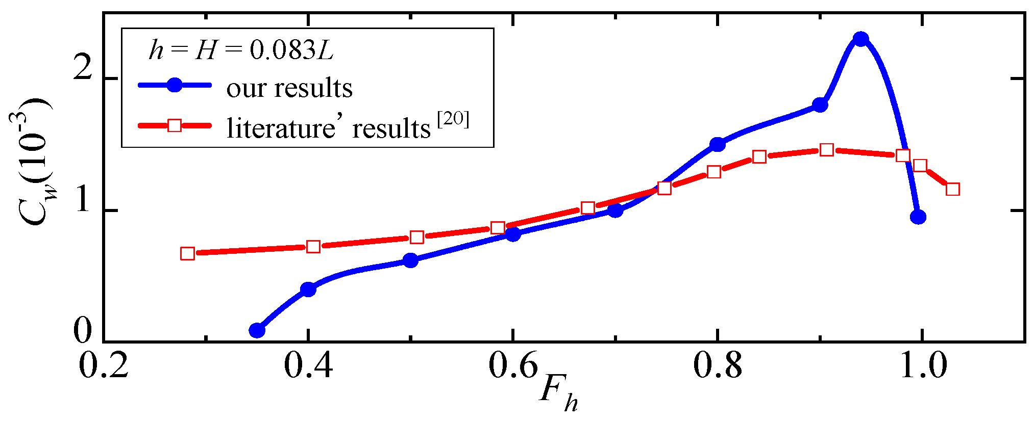
4. Validation and Results

Firstly, since the analytical solution of the ship hydrodynamic pressure field for a mixed flow is divided into two intervals, the continuity of solution between the two intervals needs to be validated. Secondly, for a sub-subcritical mixed flow, since ${\beta }_1/{\gamma }_1<k<{\beta }_2/{\gamma }_2$ and the denominator of the above analytical solution exits zero, there is serious singularity for calculation, which poses a great mathematical difficulty in solving the solution. Therefore, the validation of analytical solution is carried out by simplifying to a simple water, that is, simplifying the non-uniform water depth case to a uniform water depth case, such as open sea and rectangular channel, etc., and further comparing the calculated results with available data. The details of ship A and ship B for validation are shown in the

Table 1. The details of ship A and ship B for validation.

Dimensionless Parameters	Ship A	Ship B
Ship length between perpendiculars	1	1
Ship breadth	0.133	0.20
Ship draft	0.021	0.052
Block coefficient	0.60	0.46

. Ship A is used to carry out the validation of the wave resistance, which can also indirectly validate the analytical solution of pressure field in open sea, and ship B is used to validate the analytical solution of pressure field in rectangular channel. Since the analytical method is based on the thin-ship assumption of Wigley mathematical ship, there are some differences in ship shapes between the calculated ships and the validated ships, whose main scales are the same.

4.1. Continuity Validation

As y = w₁, where it is at the intersection of the inner and outer domains, substituting y = w₁ into Equation (40) of the velocity field and Equation (41) of the pressure field, we can then obtain that,

$$\varphi (x,w_1-0)=\mathit{\Phi }(x,w_1+0)\mathrm{and}{C}_p(x,w_1-0)=C_p(x,w_1+0)$$

(43)

which confirms that the velocity potential and the pressure coefficient of y=w₁ obtained by the inner part of Equations (40) and (41) are both the same as those obtained by the outer part of Equations (40) and (41), respectively, and further indirectly validate the analytical solution of the ship hydrodynamic pressure field.

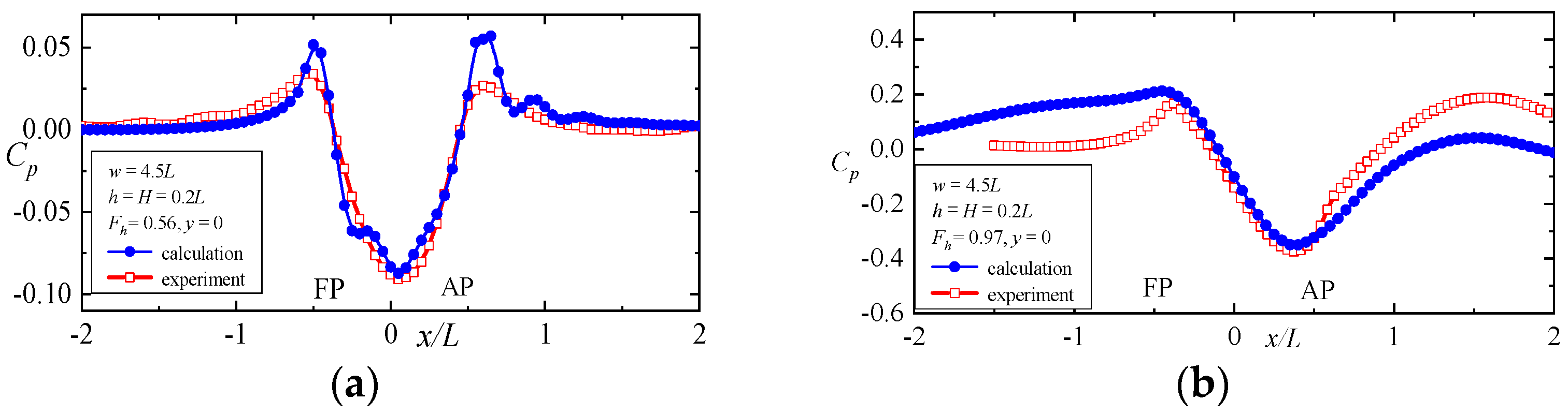
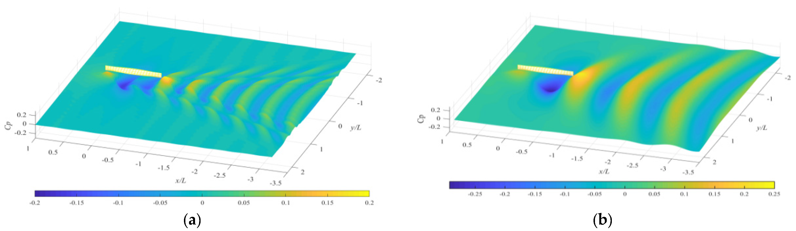
4.2. Simplify to Open Sea

Supposing there is the same depth in the inner and outer domains, that is, h=H, then ${\beta }_1={\beta }_2$, ${\gamma }_1={\gamma }_2$, $t_1=t_2=i{s}_1$, $s_1=s_2$, $d_1=1$, $r_1=1$, $q_1=i$. Thus, the complex restricted waters are simplified to the open sea with the same depth, that is, a sub-subcritical mixed flow is simplified to a simple subcritical flow, and the inner part of Equation (41) can be simplified to:

$$C_p(x,y)={\displaystyle \underset{0}{\overset{\infty }{\int }}g(k,y)}\mathrm{d}k\mathrm{as}y\le w_1$$

(44)

where if $0<k<{\beta }_1/{\gamma }_1$, $g(k,y)=-\frac{2k^2\tilde{f}(k)}{\pi }\frac{\sinh [(w_1-y)t_1]+\cosh [(w_1-y)t_1]}{t_1[\cosh (w_1{t}_1)+\sinh (w_1{t}_1)]}\cos (kx)$; if ${\beta }_1/{\gamma }_1<k$, $g(k,y)=-\frac{2k^2\tilde{f}(k)}{\pi }\frac{\sin [(w_1-y)s_1]\cos (kx)\cos (w_1{s}_1)-\sin (kx)\cos (y{s}_1)}{s_1}$ $+\frac{2k^2\tilde{f}(k)}{\pi }\frac{\cos [(w_1-y)s_1]\cos (kx)\sin (w_1{s}_1)}{s_1}$.

Furthermore, we can obtain:

$$C_p(x,y)={\displaystyle \underset{0}{\overset{\infty }{\int }}g(k,y)}\mathrm{d}k\mathrm{as}y\le w_1$$

(45)

where if $0<k<{\beta }_1/{\gamma }_1$, $g(k,y)=-\frac{2k^2\tilde{f}(k)}{\pi }\frac{\cos (kx)e^{-y{t}_1}}{t_1}$; if ${\beta }_1/{\gamma }_1<k$, $g(k,y)=-\frac{2k^2\tilde{f}(k)}{\pi }\frac{\sin (kx+y{s}_1)}{s_1}$.

In the same way, the outer part of Equation (41) is simplified to:

$$C_p(x,y)={\displaystyle \underset{0}{\overset{\infty }{\int }}G(k,y})\mathrm{d}k\mathrm{as}y\ge w_1$$

(46)

where if $0<k<{\beta }_1/{\gamma }_1$, $G(k,y)=-\frac{2k^2\tilde{f}(k)}{\pi }\frac{\cos (kx)e^{-y{t}_1}}{t_1}$; if ${\beta }_1/{\gamma }_1<k$, $G(k,y)=-\frac{2k^2\tilde{f}(k)}{\pi }\frac{\sin (kx+y{s}_1)}{s_1}$.

Thus, it can be seen that Equations (45) and (46) obtained by simplifying are consistent with that of a simple subcritical flow in open sea [16].

Equation (45) or Equation (46) and Equation (42) are used to obtain the pressure field around the ship and calculate the wave resistance in the open sea, based on the ship A data. The wave resistance C_w at different Froude numbers of h = 0.083L is calculated and compared with the literature results [20] of the Green–Naghdi equation. Figure 4 shows that the changing trend of C_w with F_h obtained by the two methods is basically the same, that is, as F_h < 1, the wave resistance increases slowly with the speed increasing, and then near F_h = 1, the wave resistance decreases suddenly, which can indirectly validate the correctness of the analytical solution. However, the analytical modeling method developed in this paper has ignored the nonlinear effect, and simplified the ship shape, which may result in less accurate prediction of the wave resistance at some speeds, especially, near F_h = 1.

4.3. Simplify to Rectangular Channel

Supposing the outer water depth is $H\to 0$, we can obtain ${\gamma }_2=0$, $d_1=0$, $r_1=0$, $q_1=0$, $t_1=k\sqrt{{\beta }_1^2-{\gamma }_1^2{k}^2}$, $s_1=k\sqrt{{\gamma }_1^2{k}^2-{\beta }_1^2}$. Thus, complex restricted waters can be simplified to a rectangular channel with the same depth, that is, a sub-subcritical mixed flow is simplified to a simple subcritical flow, and the inner part of Equation (41) can be simplified to

$$C_p(x,y)={\displaystyle \underset{0}{\overset{\infty }{\mathrm{\int }}}g(k,y)}\mathrm{d}k\mathrm{as}y\le w_1$$

(47)

where if $0<k<{\beta }_1/{\gamma }_1$, $g(k,y)=-\frac{2k^2\tilde{f}(k)}{\pi }\frac{\cosh [(w_1-y)t_1]}{t_1\sinh (w_1{t}_1)}\cos (kx)$; if ${\beta }_1/{\gamma }_1<k$, $g(k,y)=\frac{2k^2\tilde{f}(k)}{\pi }\frac{\cos [(w_1-y)s_1]}{s_1\sin (w_1{s}_1)}\cos (kx)$.

Equation (47) is used to calculate the ship hydrodynamic pressure field on the bottom, and the calculated results were compared with the experimental results of the literature [14,15,16], based on the ship B data. The ship longitudinal pressure curves at y=0 are shown in Figure 5, which presents that the calculated and experimental curves are more consistent, meanwhile, the magnitude and location of the calculated negative peak are very close to the experimental data. However, there are some differences between their positive peaks, because the calculation is based on a pointy-tailed Wigley ship, but the experiment is based on a square-tailed ship.

Meanwhile, the three-dimensional distribution of ship hydrodynamic pressure field at different speeds is calculated and shown in Figure 6. It can be seen that the pressure field at F_h = 0.56 presents a combination of transverse and dispersive wave characteristics, but as the speed increases to F_h = 0.8, the negative peak gradually moves towards the ship stern and the pressure field mainly presents transverse wave characteristics. Thus, it is obvious that there are differences in the characteristics of the ship hydrodynamic pressure field at different speeds

5. Conclusions

The main aim of this study was to develop a mathematical modeling method for studying the analytical solution of the ship hydrodynamic pressure fields in complex restricted waters. Based on the potential flow theory and the thin-ship assumption, dividing complex restricted waters with varying depths into the inner and outer domains with constant depths, a mathematical modeling method can be developed and carried out for analyzing and solving the partial differential equations consisting of the governing equation with a dispersion effect and boundary conditions. Meanwhile, the research indicates that the partition of integral intervals plays an important role in the research, and the mathematical modeling for different mixed flows needs to be studied separately for multiple integral intervals due to the difference in mathematical characteristics. In this paper, the analytical solution for a sub-subcritical mixed flow is obtained by the mathematical modeling method and validated by simplifying to a simple water; however, because of the large singularity of calculation in range ${\beta }_1/{\gamma }_1<k$, the key technological challenge for solving the analytical solution has not yet been completely overcome, while the key challenge for sub-supercritical or super-supercritical mixed flow had been successfully overcome [17,18]. Thus, future effort for solving the sub-subcritical analytical solution is still needed, although there is great technical difficulty in solving the singularity problem.

In addition, the mathematical modeling method, as well as the analytical solution proposed in this paper, can provide references for related studies in more complex restricted waters, such as trapezoidal channels, etc., and are also of great academic value for application in mathematics, military, and engineering fields.

References

1. Jiang, M. Waterway Engineering; China Water Conservancy and Hydropower Press: Beijing, China, 2009; pp. 11–18. [Google Scholar]
2. Zhang, W. Effects of shallow waters effects on ships and empirical estimation methods. Ship Mar. Eng. 2019, 35, 6–12. [Google Scholar]
3. Ni, H.; She, H.Q. Status and development trend of foreign submarine mines. Mine Warfare Ship Protect. 2013, 21, 1–8. [Google Scholar]
4. Tuck, E.O. Shallow-water flows past slender bodies. J. Fluid Mech. 1966, 26, 81–95. [Google Scholar] [CrossRef]
5. Tuck, E.O. Hydrodynamic Problems of Ships in Restricted Waters. Annu. Rev. Fluid Mech. 1978, 10, 33–46. [Google Scholar] [CrossRef]
6. Tuck, E.O. Bottom Pressure Signatures; Department of Applied Mathematics, The University of Adelaide: Adelaide, Australia, 1998. [Google Scholar]
7. Terziev, M.; Tezdogan, T.; Oguz, E.; Gourlay, T.; Demirel, Y.K.; Incecik, A. Numerical investigation of the behaviour and performance of ships advancing through restricted shallow waters. J. Fluids Struct. 2018, 76, 185–215. [Google Scholar] [CrossRef] [Green Version]
8. Tafuni, A.; Sahin, I. Seafloor Pressure Signatures of a High-Speed Boat in Shallow Water With SPH. In Proceedings of the ASME 2014 33rd International Conference on Ocean, Offshore and Arctic Engineering, San Francisco, CA, USA, 8–13 June 2014; American Society of Mechanical Engineers: New York, NY, USA, 2014. OMAE2014-24080. [Google Scholar] [CrossRef]
9. Tafuni, A.; Sahin, I.; Hyman, M. Numerical investigation of wave elevation and bottom pressure generated by a planing hull in finite-depth water. Appl. Ocean Res. 2016, 58, 281–291. [Google Scholar] [CrossRef]
10. Veen, D.; Gourlay, T. A combined strip theory and Smoothed Particle Hydrodynamics approach for estimating slamming loads on a ship in head seas. Ocean Eng. 2012, 43, 64–71. [Google Scholar] [CrossRef] [Green Version]
11. Gourlay, T.P. A brief history of mathematical ship-squat prediction, focussing on the contributions of EO Tuck. J. Eng. Math. 2011, 70, 5–16. [Google Scholar] [CrossRef]
12. Gourlay, T.P. Shallow Flow: A Program to Model Ship Hydrodynamics in Shallow Water. In Proceedings of the ASME 2014 33rd International Conference on Ocean, Offshore and Arctic Engineering, San Francisco, CA, USA, 8–13 June 2014. [Google Scholar]
13. Gourlay, T.P.; Jeong, H.H.; Philipp, M. Sinkage and trim of modern container ships in shallow water. In Proceedings of the Australasian Coasts & Ports Conference, Auckland, New Zealand, 15–18 September 2015. [Google Scholar]
14. Hui, D.; Zhi-Hong, Z.; Ju-Bin, L.; Jian-Nong, G. Research on the calculation method of pressure field for shallow water subcritical speed ships. J. Appl. Math. Mech. 2013, 34, 846–854. [Google Scholar]
15. Hui, D.; Zhi-Hong, Z.; Jian-Nong, G.; Ju-Bin, L. Hydrodynamic pressure field caused by a ship sailing near the coast. J. Coast. Res. 2016, 32, 890–897. [Google Scholar]
16. Sun, B.B.; Zhi-Hong, Z.; Ju-Bin, L.; Hui, D. The theoretical solution and calculation of the hydrodynamic pressure field of ship in the shallow channel. Ship Sci. Technol. 2014, 36, 11–16. [Google Scholar]
17. Zhi-Hong, Z.; Hui, D.; Chong, W. Analytical models of sub-supercritical ship hydrodynamic pressure field with the dispersive effect. Ocean Eng. 2017, 133, 66–72. [Google Scholar] [CrossRef]
18. Qing-Chang, M.; Hui, D.; Zhi-Hong, Z. Analytical models of ship hydrodynamic pressure field with dispersive effect in super-supercritical mixed flow. Ocean Eng. 2018, 167, 95–101. [Google Scholar]
19. Xue-Nong, C.; Sharma, S.D. A slender ship moving at a near-critical speed in a shallow channel. J. Fluid Mech. 1995, 291, 263–285. [Google Scholar]
20. Bo, C. Numerical Studying of Ship Waves in Shallow Water based on Green-Naghdi Equations; Huazhong University of Science and Technology: Wuhan, China, 2004. [Google Scholar]
Figure 1. The coordinate system for a ship advancing in complex restricted waters: (a) dredged channel ;(b) trapezoidal channel.
Jmse 10 00232 g001
Figure 2. The research content related to the mathematical modeling, which is divided into two cases: simple restricted waters and complex restricted waters; and this paper focuses on the complex restricted waters.
Jmse 10 00232 g002
Figure 3. The sketch of the mathematical modeling method for complex restricted waters.
Jmse 10 00232 g003
Figure 4. The comparisons between the wave resistances of our and literature [20]’s calculations.
Jmse 10 00232 g004
Figure 5. The comparisons of the ship longitudinal pressure curves on the sea bottomh(y = 0): (a) calculated data vs. experimental data of Fh = 0.56; (b) calculated data vs. experimental data of Fh = 0.967.
Jmse 10 00232 g005
Figure 6. The three-dimensional distribution of ship hydrodynamic pressure field on the sea bottom (h = H = 0.2L): (a) calculated data of Fh = 0.56; (b) calculated data of Fh = 0.8.
Jmse 10 00232 g006