Author Contributions
Conceptualization, M.S.J.; methodology, M.S.J. and J.K.M.; formal analysis, M.S.J.; data curation, M.S.J.; writing—original draft preparation, M.S.J.; writing—review and editing, J.K.M.; visualization, M.S.J.; supervision, J.K.M.; project administration, J.K.M. All authors have read and agreed to the published version of the manuscript.
Figure 1.
Study area location. Alternating red and yellow lines depict NJ Shoreline Segments utilized by Lemke and Miller [
38] to produce the storm erosion potential climatology. Segments are numbered from north to south with #1 at Sandy Hook and #13 at Cape May. NJ coastal are counties labeled accordingly. Black + markers depict NJBPN survey locations. Map coordinate system is NAD83/UTM Zone 18N in kilometers. Courtesy of [
20].
Figure 2.
Spatial variance for select Resilience parameters by segment. (
a) Dune crest elevation; (
b) Dune volume; (
c) Berm width; (
d) Beach slope. Presented by segment, south (13) to north (1). Red horizontal bar—median value, blue box—25th and 75th percentiles. Outliers defined by 1.5 × IQR away from 25th/75th percentiles. Courtesy of [
48].
Figure 3.
Aggregated summary of quantity of profiles available and corresponding dune volume loss percentage by storm for the New Jersey coast. Courtesy of [
20].
Figure 3.
Aggregated summary of quantity of profiles available and corresponding dune volume loss percentage by storm for the New Jersey coast. Courtesy of [
20].
Figure 4.
Conceptual flowchart to highlight sources of previously published data used to generate the EDP and subsequent fragility curves.
Figure 4.
Conceptual flowchart to highlight sources of previously published data used to generate the EDP and subsequent fragility curves.
Figure 5.
Observed dune loss percentage as a function of storm intensity (PEI) alone; each data point represents observations from a single profile. X-axis is storm intensity (PEI). Storm categories are denoted by colored vertical dashed lines. The Y-axis is dune loss percentage. Red circles indicate Major loss (>40%), blue circles indicate Moderate (>5% but <40%). Negative dune loss indicates accretion.
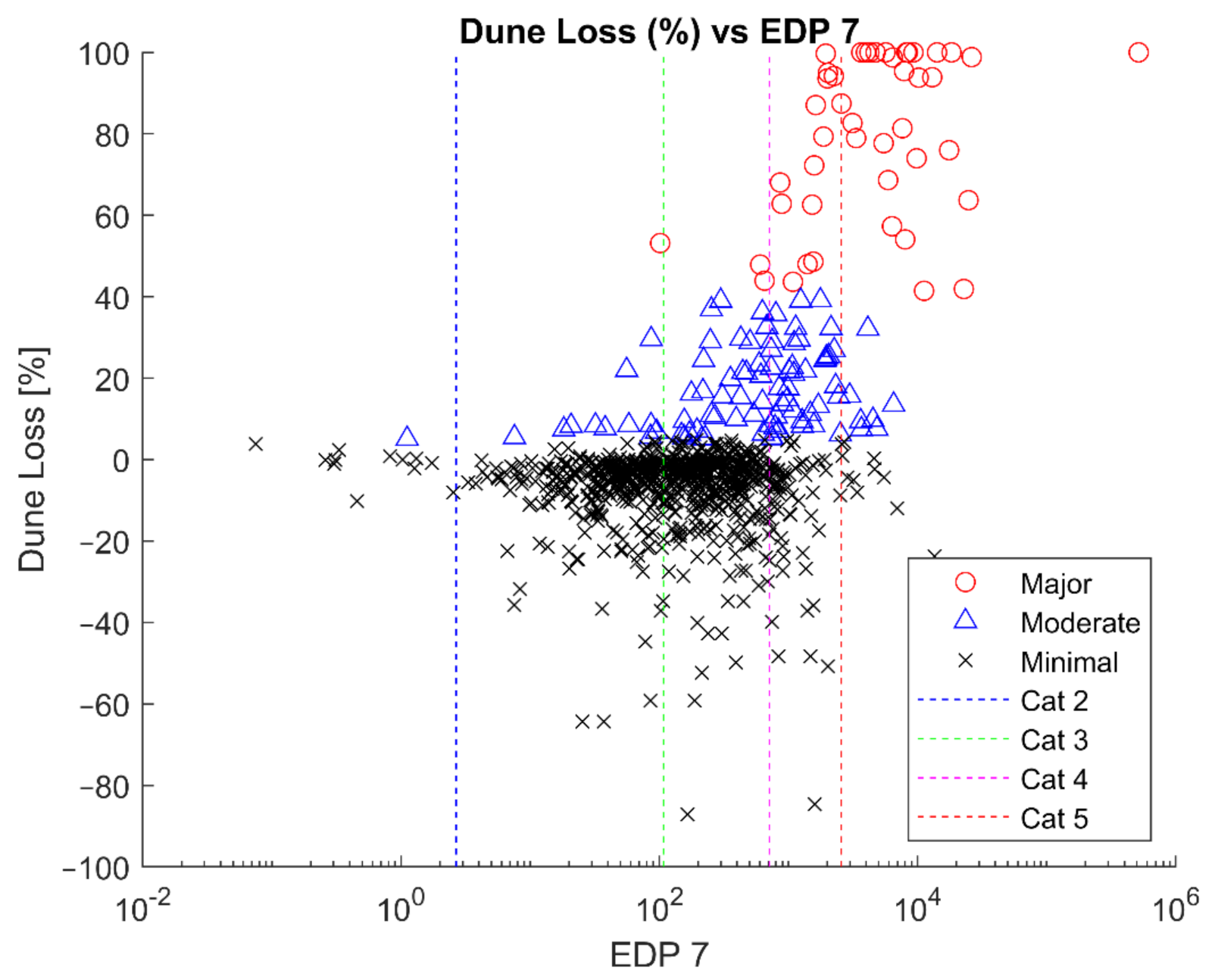
Figure 6.
Observed dune loss percentage as a function of EDP Case 7; each data point represents observations from a single profile. X-axis is the EDP. Storm categories are denoted by colored vertical dashed lines. Storm category PEI values converted to an EDP using median resilience parameters. The Y-axis is dune loss percentage. Red circles indicate Major loss (>40%), blue circles indicate Moderate (>5% but <40%). Negative dune loss indicates accretion.
Figure 7.
Weibull distribution quantile plots for all observations corresponding to Moderate classification. (a) EDP 1—Berm Width; (b) EDP 2—Berm and Dune width; (c) EDP 3—Dune Volume; (d) EDP 4—Foredune Volume; (e) EDP 5—Shear; (f) EDP 6—Moment; (g) EDP 7—Simplified Mass-moment of Inertia; (h) EDP 8—Mass-moment of Inertia.
Figure 8.
Weibull distribution quantile plots for all observations corresponding to Major classification. (a) EDP 1—Berm Width; (b) EDP 2—Berm and Dune width; (c) EDP 3—Dune Volume; (d) EDP 4—Foredune Volume; (e) EDP 5—Shear; (f) EDP 6—Moment; (g) EDP 7—Simplified Mass-moment of Inertia; (h) EDP 8—Mass-moment of Inertia.
Figure 9.
Weibull distribution quantile plots removing maximum observation corresponding to Major classification with a single datapoint removed. Only EDP cases 5 to 8 are shown for clarity. (a) EDP 5—Shear; (b) EDP 6—Moment; (c) EDP 7—Simplified Mass-moment of Inertia; (d) EDP 8—Mass-moment of Inertia.
Figure 10.
Example log-normal distribution for EDP 7 for calibration/training (triangular shapes) and test datasets (square/diamond). Dashed curves represent MLE log-normal fit curves with red denoting Major and blue denoting Moderate classification.
Figure 10.
Example log-normal distribution for EDP 7 for calibration/training (triangular shapes) and test datasets (square/diamond). Dashed curves represent MLE log-normal fit curves with red denoting Major and blue denoting Moderate classification.
Figure 11.
Comparation of Weibull (solid line) vs. log-normal distribution (dashed) for EDP 7. Observed fractions of classification are denoted by shapes and retained from previous figure to illustrate performance. Red denotes Major, Blue denotes Moderate classification.
Figure 11.
Comparation of Weibull (solid line) vs. log-normal distribution (dashed) for EDP 7. Observed fractions of classification are denoted by shapes and retained from previous figure to illustrate performance. Red denotes Major, Blue denotes Moderate classification.
Figure 12.
Log-normal predicted and observed fractions of damage classification by storm category (vertical columns). Each subplot corresponds to a damage classification: (a) Minimal; (b) Moderate; (c) Major. Vertical bars correspond to EDP case (1 to 8 in each box), whiskers are standard deviation in predicted probabilities for storms within the Category. Dashed red horizontal bar is the fraction of observed classifications corresponding to the appropriate storm category.
Figure 13.
Comparison of Weibull (green/right) and log-normal (blue/left) models by storm category (vertical columns). Each subplot corresponds to a damage classification: (a) Minimal; (b) Moderate; (c) Major. Each vertical bar corresponds to an EDP case and model. Note only EDPs 5–8 are shown. Whiskers are standard deviation in predicted probabilities for the corresponding category of storms. Dashed red horizontal bar is the actual observed fraction corresponding to the appropriate storm category.
Table 1.
Summary of available measures of Storm Intensity and key characteristics. Note variables are identified in ‘Parameters Considered’ column.
Table 1.
Summary of available measures of Storm Intensity and key characteristics. Note variables are identified in ‘Parameters Considered’ column.
| Parameter | Storm Type | Intensity Measure | Equation | Output | Units | Parameters Considered | Source |
|---|
| Saffir–Simpson Hurricane Wind Scale | Tropical | Peak | N/A | Category (1–5) | - | Windspeed | Schott et al. (2012) [26] |
| Hurricane Intensity Index (HII) & Hurricane Hazard Index (HHI) | Tropical | Peak |
| - | - | Windspeed (V), Radius (R) and translation speed (S), 0 designates reference values | Kantha (2006) [27] |
| Integrated Kinetic Energy (IKE) | Tropical | Peak | | - | - | Wind speed (U), Storm Volume (V) | Powell and Reinhold (2007) [28] |
| Hurricane Severity Index | Tropical | Peak | Size + Intensity | 50-point scale | - | Wind speed, Radius | Hebert et al. (2010) [29] |
| Surge Scale (SS) | Tropical | Peak | | surge | m | ) | Irish and Resio (2010) [30] |
| Cyclone Damage Potential Index (CDP) | Tropical | Peak | | - | - | Wind speed (vm), Radius (Rh), forward speed (vt) | Done et al. (2015) [31] |
| Dolan and Davis Scale | Extra-tropical | Peak | | - | m2-s | Wave Height (Hs) duration (td) | Dolan and Davis (1992) [32] Mendoza et al. (2011) [33] |
| Shoreline Risk Index | Extra-tropical | Peak | | - | m2-s0.3 | Wave height (H), Surge (S), number of tidal cycles (tD) | Kriebel et al. (1996) [22] |
| Storm Erosion Potential Index (SEIP) | Extra-tropical | Cumulative | | - | m3 | Storm surge (S and H), tide duration (t) | Zhang et al. (2001) [34] |
| Balsillie Regression Analysis | Both | Peak | | Volume (Q) | m3 | Surge (S), Tide Rise (tr) | Balsillie (1986) [35] |
| Maximum Wave Run-up (Rmax) | Both | Peak |
| Wave Run-up (R) | m | ) | Kraus and Wise (1993) [36] |
| Coastal Storm Impulse Parameter (COSI) | Both | Cumulative | | Impulse (Is) | kg-s per m | Total Horizontal momentum, surge (fp(t)) and Wave (M(t)) (wave height, period, surge, duration) | Basco and Mhmoudpour (2012) [25] |
| Storm Erosion Potential Index | Both | Both | | cross-shore distance | m | Water level (S), wave height (Hb) and duration (t), Berm elevation (B) | Miller and Livermont (2008) [37] Lemke and Miller (2020) [38] |
Table 2.
Average SEI and PEI values, and associated return periods (
tr), for eighteen historical storms in New Jersey. Storm data from [
20]. Return periods are based on frequency of occurrence curves by [
49].
Table 2.
Average SEI and PEI values, and associated return periods (
tr), for eighteen historical storms in New Jersey. Storm data from [
20]. Return periods are based on frequency of occurrence curves by [
49].
| Event | SEI | SEI tr [yr] | PEI | PEI tr [yr] |
|---|
| October 1991 | 1534 | 5.2 | 67.3 | 5.2 |
| January 1992 | 1017 | 2.2 | 64.4 | 4.1 |
| December 1992 | 3326 | 24 | 90.8 | 20 |
| December 1994 | 869 | 1.7 | 57.5 | 2.3 |
| January 1996 | 719 | 1.3 | 51.1 | 1.4 |
| February 1998 | 1434 | 4.5 | 67.0 | 5.0 |
| September 2003 | 1040 | 2.3 | 53.8 | 1.8 |
| 12 October 2005 | 1779 | 6.8 | 54.3 | 1.8 |
| 25 October 2005 | 866 | 1.7 | 60.0 | 1.4 |
| September 2006 | 964 | 2.0 | 50.3 | 1.4 |
| November 2007 | 670 | 1.2 | 60.4 | 2.9 |
| May 2008 | 998 | 2.1 | 53.4 | 1.7 |
| September 2008 | 1714 | 6.4 | 54.3 | 1.8 |
| November 2009 (Vets) | 2986 | 18 | 74.8 | 9.1 |
| March 2010 | 1220 | 3.2 | 58.7 | 2.5 |
| September 2010 | 581 | 1.0 | 62.9 | 3.6 |
| August 2011 (Irene) | 788 | 1.4 | 73.3 | 8.2 |
| October 2012 (Sandy) | 3056 | 19 | 119 | 49 |
Table 3.
Storm Categories based on SEI and PEI including parameter value, return period (Tr) and annual probability of exceedance. Storm categories determined by [
38], return period calculated from [
49].
Table 3.
Storm Categories based on SEI and PEI including parameter value, return period (Tr) and annual probability of exceedance. Storm categories determined by [
38], return period calculated from [
49].
| | SEI | PEI |
|---|
| Category | Value | Tr | Annual Prob. | Value | Tr | Annual Prob. |
|---|
| 2 | 730 | 1 | 77.1% | 23 | <1.0 | >99.9% |
| 3 | 1510 | 5 | 19.8% | 58 | 2 | 41.5% |
| 4 | 2300 | 10 | 9.5% | 93 | 22 | 4.7% |
| 5 | 3080 | 19 | 5.2% | 128 | 62 | 1.6% |
Table 4.
Reduced parameters of interest. Note FB denotes freeboard or vertical distance between parameter and mean sea level, WL—water level, vol—volume, Hb—breaking wave height, cumE—cumulative energy (H2), Z denotes elevation, Max denotes the maximum hourly value over a single storm duration and Bslope/Islope denote beach and intertidal slope.
| Type | Parameter Name | Symbol/Abbreviation | Units | Highly Correlated |
|---|
| Intensity Measure | Peak Erosion Intensity | PEI | Length (m) | MaxWL, MaxHb, cumE, DL, DLvol |
| Resilience | Berm Width | Bwidth | Length (m) | Berm Vol |
| Resilience | Crest Width (cross-shore distance from dune toe to crest) | Fwidth | Length (m) | Fvol, Dvol, Fslope−1 |
| Resilience | Dune volume (volume from toe to heel) | Dvol | Volume per length (m3/m) | CrestZ, ToeZ, CrestFB |
| Resilience | Foredune volume (volume from toe to crest) | Fvol | Volume per length (m3/m) | Fwidth, CrestZ, Dvol, CrestFB, Fslope−1 |
| Resilience | Dune Crest Elevation | CrestZ | Length (m) | Dvol, Fvol, ToeZ, CrestFB, ToeFB, Bslope, |
| Resilience | Dune Toe Elevation | ToeZ | Length (m) | CrestFB, ToeFB, d50, ISlope, BSlope, CrestZ |
| Impact | Dune Loss Percent | DL | % (-) | DLvol |
Table 5.
Considered EDPs, underlying parameters (IM and Rf) and physical meaning.
Table 5.
Considered EDPs, underlying parameters (IM and Rf) and physical meaning.
| Case | Parameters | EDP | Physical Proxy |
|---|
| 1 | PEI, Berm Width | | Setback |
| 2 | PEI, Berm Width, Dune Crest Width | | Setback |
| 3 | PEI, Dune Volume | | Volume |
| 4 | PEI, Foredune Volume | | Volume | ‘540-rule’ |
| 5 | PEI, Berm Width and Dune Volume | | Shear |
| 6 | PEI, Berm Width and Dune Volume | | Moment |
| 7 | PEI, Berm Width and Dune Volume | | Simplified Mass-moment of Inertia |
| 8 | PEI, Berm Width and Dune Volume | | Mass-moment of Inertia |
Table 6.
Classification of storm-induced dune impacts based on quantitative changes.
Table 6.
Classification of storm-induced dune impacts based on quantitative changes.
| Damage Class | Definition |
|---|
| Major | Dune volume loss > 40% |
| Moderate | Dune volume loss 5–40% |
| Minor | Dune volume loss < 5% |
Table 7.
Best Estimate Normal Distribution parameters.
Table 7.
Best Estimate Normal Distribution parameters.
| EDP | Moderate | Major |
|---|
| θ (Median) | β (Dispersion) | θ (Median) | β (dispersion) |
|---|
| 5 | 1220 | 1.80 | 2058 | 1.10 |
| 6 | 702 | 1.51 | 1694 | 1.15 |
| 7 | 1839 | 1.99 | 45629 | 2.50 |
| 8 | 1260 | 2.34 | 7915 | 2.05 |
Table 8.
Best Estimate Weibull Distribution parameters.
Table 8.
Best Estimate Weibull Distribution parameters.
| EDP | Moderate | Major |
|---|
| λ (Scale) | κ (Shape) | λ (Scale) | κ (Shape) |
|---|
| 5 | 366 | 1.30 | 635 | 3.04 |
| 6 | 282 | 1.78 | 1012 | 2.16 |
| 7 | 570 | 1.14 | 4428 | 1.32 |
| 8 | 243 | 1.13 | 1697 | 1.35 |
Table 9.
Error metrics for log-normal MSA curves.
Table 9.
Error metrics for log-normal MSA curves.
| | MAE | Bias | RMSE |
|---|
| | Moderate | Major | Moderate | Major | Moderate | Major |
|---|
| 1 | 26% | 16% | −21% | −16% | 35% | 26% |
| 2 | 23% | 13% | −19% | −13% | 30% | 20% |
| 3 | 26% | 17% | −19% | −16% | 32% | 24% |
| 4 | 26% | 15% | −19% | −14% | 33% | 21% |
| 5 | 25% | 16% | −20% | −16% | 33% | 25% |
| 6 | 15% | 9% | −11% | −8% | 19% | 12% |
| 7 | 15% | 18% | −12% | −18% | 19% | 28% |
| 8 | 19% | 15% | −16% | −15% | 25% | 22% |


