Abstract
This paper presents the development of a low-energy passive acoustic vessel detector to work as part of a wireless underwater monitoring network. The vessel detection method is based on a low-energy implementation of Detection of Envelope Modulation On Noise (DEMON). Vessels produce a broad spectrum modulated noise during propeller cavitation, which the DEMON method aims to extract for the purposes of automated detection. The vessel detector design has different approaches with mixtures of analogue and digital processing, as well as continuous and duty-cycled sampling/processing. The detector re-purposes an existing acoustic modem platform to achieve a low-cost and long-deployment wireless sensor network. This integrated communication platform enables the detector to switch between detection/communication mode seamlessly within software. The vessel detector was deployed at depth for a total of 84 days in the North Sea, providing a large data set, which the results are based on. Open sea field trial results have shown detection of single and multiple vessels with a 94% corroboration rate with local Automatic Identification System (AIS) data. Results showed that additional information about the detected vessel such as the number of propeller blades can be extracted solely based on the detection data. The attention to energy efficiency led to an average power consumption of 11.4 mW, enabling long term deployments of up to 6 months using only four alkaline C cells. Additional battery packs and a modified enclosure could enable a longer deployment duration. As the detector was still deployed during the first UK lockdown, the impact of COVID-19 on North Sea fishing activity was captured. Future work includes deploying this technology en masse to operate as part of a network. This could afford the possibility of adding vessel tracking to the abilities of the vessel detection technology when deployed as a network of sensor nodes.
1. Introduction
Our oceans cover more than 70% of the world’s surface and for island nations such as the United Kingdom (UK), this can result in a large amount of coastline being vulnerable if not effectively monitored [1]. Some examples of coastline vulnerabilities can include drug and human trafficking, military threats, and illegal fishing activity [2,3,4,5,6,7,8]. The English channel would be incredibly difficult to monitor 24 h a day, especially at night and in poor weather conditions. The English channel spans approximately 75,000 km2 and weather conditions can be extreme, especially during the winter months [9]. To monitor such a large area in all conditions using sea- and air-based vehicles would be challenging, incredibly labour intensive, and could carry a sizeable cost. A low-cost alternative to detect surface vessels could help to address some of the examples illustrated for monitoring ocean activity.
One piece of relatively low-cost technology currently available, and in the most part widely adopted, is the Automatic Identification System (AIS). AIS uses transponders for the tracking of vessel activity by relaying data such as position, course, and speed [10]. However, the AIS system is not legally required for all vessel types and it is highly unlikely that other vessels acting illegally will adopt this technology [11]. In the examples of human trafficking cited, the vessels used tend to be small rigid hulled inflatable boats (RHIB), which, due to their low radar signature and lack of an AIS transponder, are very hard to spot optically in poor weather. However, one feature that a motor-powered vessel cannot hide in any atmospheric condition is the noise that is produced by the vessel itself during navigation.
It should be declared that this paper reuses some content from the thesis ‘Low Energy, Passive Acoustic Sensing for Wireless Underwater Monitoring Networks’, with permission [12].
1.1. Propeller Cavitation
Vessels can produce noise from a variety of sources including propeller, electric motors, diesel generators, auxiliary machinery, and water flow [13]. The most intense source of noise tends to stem from a vessel’s propeller [14]. As a propeller rotates through the water, tiny bubbles of air are formed and consequently collapse under the pressure of the surrounding water. This collapse creates a pressure wave in the water, which is the noise we associate with the propeller. This process is known as propeller cavitation. It should be noted that cavitation only occurs when the propeller creates sufficiently low pressure to cause bubbles to form and collapse [15]. Therefore, a propeller rotating extremely slow or at a great depth may not cause cavitation to occur, as the pressure does not reach a low enough level for the formation of bubbles. The noise created contains a broadband high-frequency component which fluctuates in intensity in an almost rhythmic nature [15]. The envelope of the high-frequency, amplitude-modulated signal produced during propeller cavitation is proportional to the rate of rotation of the propeller. This envelope signal is a strong indicator when attempting to detect a vessel using a passive acoustic methodology. To illustrate the high-frequency noise produced during propeller cavitation, a recording has been taken for analysis, which belongs to a RHIB owned by Newcastle University. Figure 1 shows the RHIB docked at Blyth Marine station in preparation for field trials.
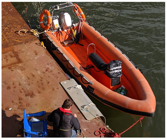
Figure 1.
Rigid Hulled Inflatable Boat (RHIB) owned by Newcastle University used during vessel detector field trial experiments.
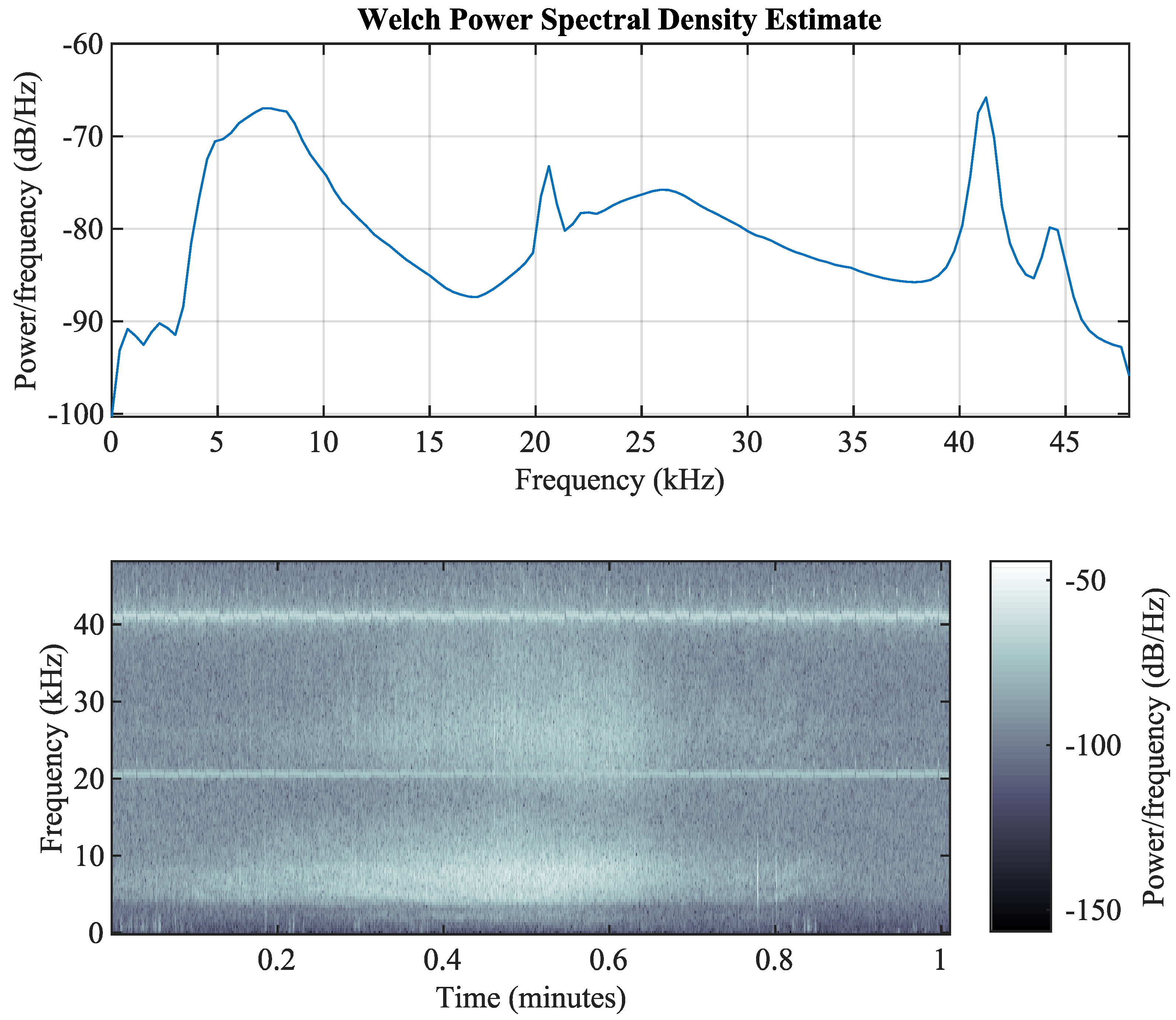
Figure 2 shows the associate spectrum captured during recording of the vessel passing. The spectrum shows that the RHIB’s cavitation noise contains fairly broadband high-frequency components centred around 7 kHz and 26 kHz. (The sharper peaks at 21 kHz and 42 kHz stem from electrical noise within the vessel detector during recording). The next feature to exploit in passive acoustic detection of a passing vessel is to make use of the unique high-frequency fluctuation that a propeller produces during cavitation.
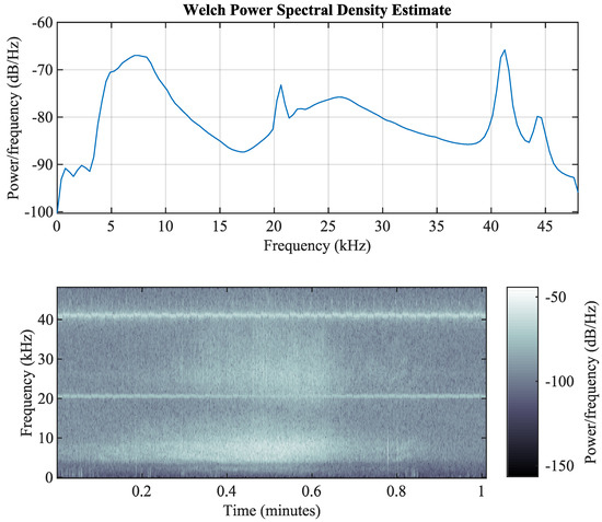
Figure 2.
Frequency spectrum of the RHIB recorded using the vessel detector’s transducer and front-end amplifier.
1.2. Passive Acoustic Vessel Detection Methods
A range of techniques have been developed in the pursuit of detecting a vessel based on its acoustic signature, many of which are introduced in Lowes et al., 2019 [16]. This section of the paper aims to provide a more in-depth review of the latest research related to passive acoustic vessel detection. It also aims to highlight the areas where this research can help to address some of the limitations others have encountered.
In its most basic form, passive acoustic vessel detection may be achieved by simply listening for a noticeable change in the background noise. A motor-powered vessel introduces noise into the water and, providing that the background noise was low prior to the vessel arriving, creates a notable change in the recorded signal energy. Listening to this signal could be enough for a human to make a judgement on whether or not a vessel was present based on the audible content. This method relies on a good signal-to-noise ratio and a skilled listener, and would ultimately be incredibly labour intensive for any prolonged monitoring period [17]. An automated electronic system would reduce the need for such a labour-intensive approach.
One method of detecting vessel activity in the presence of noise is by using a wavelet-based detection algorithm [18,19]. A Wavelet Transform (WT) provides both time and frequency information simultaneously for a given input signal as opposed to a Fourier Transform (FT), which can provide time or frequency information depending on the direction of the transform. Sorensen et al. used an energy-based detection method combined with a wavelet detection algorithm to identify vessel acoustics in the presence of background noise. The authors created a self-contained data acquisition node that is capable of capturing acoustic data for a one-month period. The data was then manually collected and analysed using the wavelet-based detection algorithm to identify the presence of vessel activity. The results of the algorithm were then compared with a human acoustic specialist. In trials this method indicated a true positive rate (TPR) of 93% for a false positive rate (FPR) of below 40% [19]. This shows a high probability of detection at the expense of a high false alarm rate. Collecting data from the deployed nodes after each one-month deployment allows for unrestricted processing power on-shore. However, for real-time critical applications such as defence, this method would not be suitable due to the delay in receiving detection results. The authors concluded that a useful area of future work would be the incorporation of this methodology into a large-scale underwater sensor network.
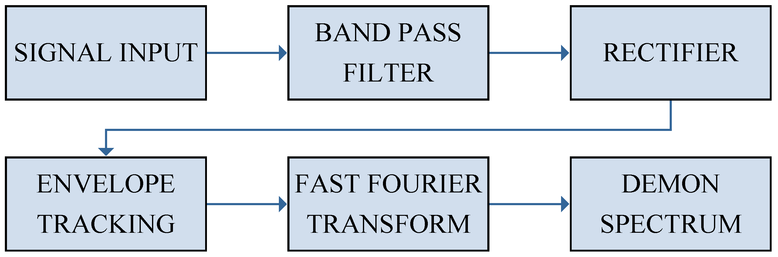
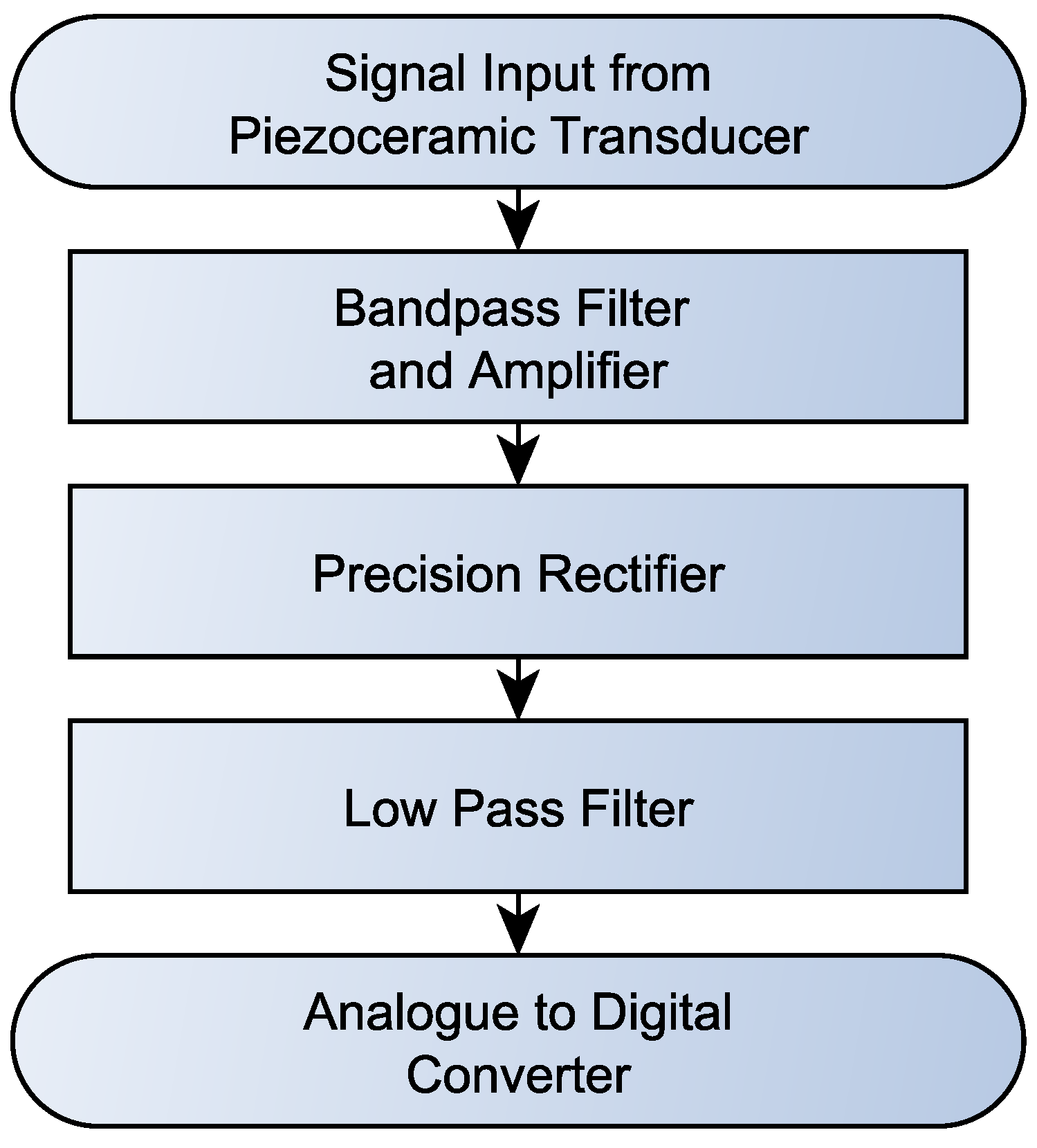
A second method that is popular amongst researchers is the Detection of Envelope Modulation On Noise or DEMON algorithm [20,21,22,23]. The basic structure of the DEMON process from a raw input signal to the final DEMON spectrum is shown in Figure 3.
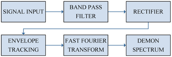
Figure 3.
Basic process of the Detection of Envelope Modulation On Noise (DEMON) algorithm. The end result produces a spectrum of the original signal envelope.
Chung et al. used the DEMON algorithm to detect ships within a busy harbour environment. The authors used a cross-correlation method from multiple hydrophone sources to establish both the ship’s bearing, but also as a tool to isolate individual ship signatures [20]. To carry out field trials of the algorithm, the authors used a piece of hardware developed by the Stevens Institute of Technology specifically for passive acoustic detection purposes. The Stevens Passive Acoustic Detection System (SPADES) consists of four hydrophones connected with a central storage and processing hub [24]. This unit is then linked via an underwater cable to a shore-side computer to provide power and communication of results. An underwater cable offers advantages such as reliability and increased processing power. The limitations may be the cost of installing such an asset, and from a defence point of view, it may be noticed by potential security threats.
Clark et al. documented another variation on the DEMON algorithm in which the acoustic signal produced by a vessel is processed using sub-band filtering. The authors showed that by using this method, the modulation harmonics related to propeller cavitation can be emphasised, improving the signal-to-noise ratio by as much as 3.2 dB [21]. This improvement comes at the expense of increased processing power given the multiple sub-band digital filters.
Pollara et al. present several improvements on the widely used DEMON algorithm for vessel detection. The author firstly used two hydrophones to indicate the Time Difference Of Arrival (TDOA) of a vessel based on phase delay. Results show that the TDOA of a vessel can be used as a method of vessel bearing tracking. Secondly the DEMON spectrums of several small vessels were collected and analysed to establish potential classification characteristics. Results showed that the number of peaks along with their magnitudes could provide a tool for classification in small vessels. Finally, the authors discussed the dependence of the DEMON algorithm on the high-frequency carrier signal it aims to demodulate. Results showed that the selection of passband for DEMON analysis has a large bearing on the success of detection and classification [22]. The authors also utilised the SPADES system developed by the Stevens Institute of Technology [24]. Sampling was set at 200 kHz to capture the high-frequency energy produced during propeller cavitation. The method described by the authors shows promising results in terms of reliability, but the high sample rate and fixed monitoring equipment limits the setup in terms of deployment location and speed of deployment. It also places much emphasis on the reliability of the SPADES system, whereas multiple redundancy may be seen as advantageous for a defence-based application.
The DEMON papers discussed demonstrate that the methodology in its most basic form is widely used and achieves strong detection results. There are many credible lines of improvement presented in the papers discussed; however, many would require significant processing and a high energy budget. As the Stevens Institute of Technologies SPADES equipment demonstrates, a permanent power cable is required when processing and communicating data in isolated underwater areas. For true effectiveness in monitoring our oceans for vessel activity, a fully wireless system capable of both detecting and communicating results could address many of the practical issues highlighted.
1.3. Underwater Sensor Network
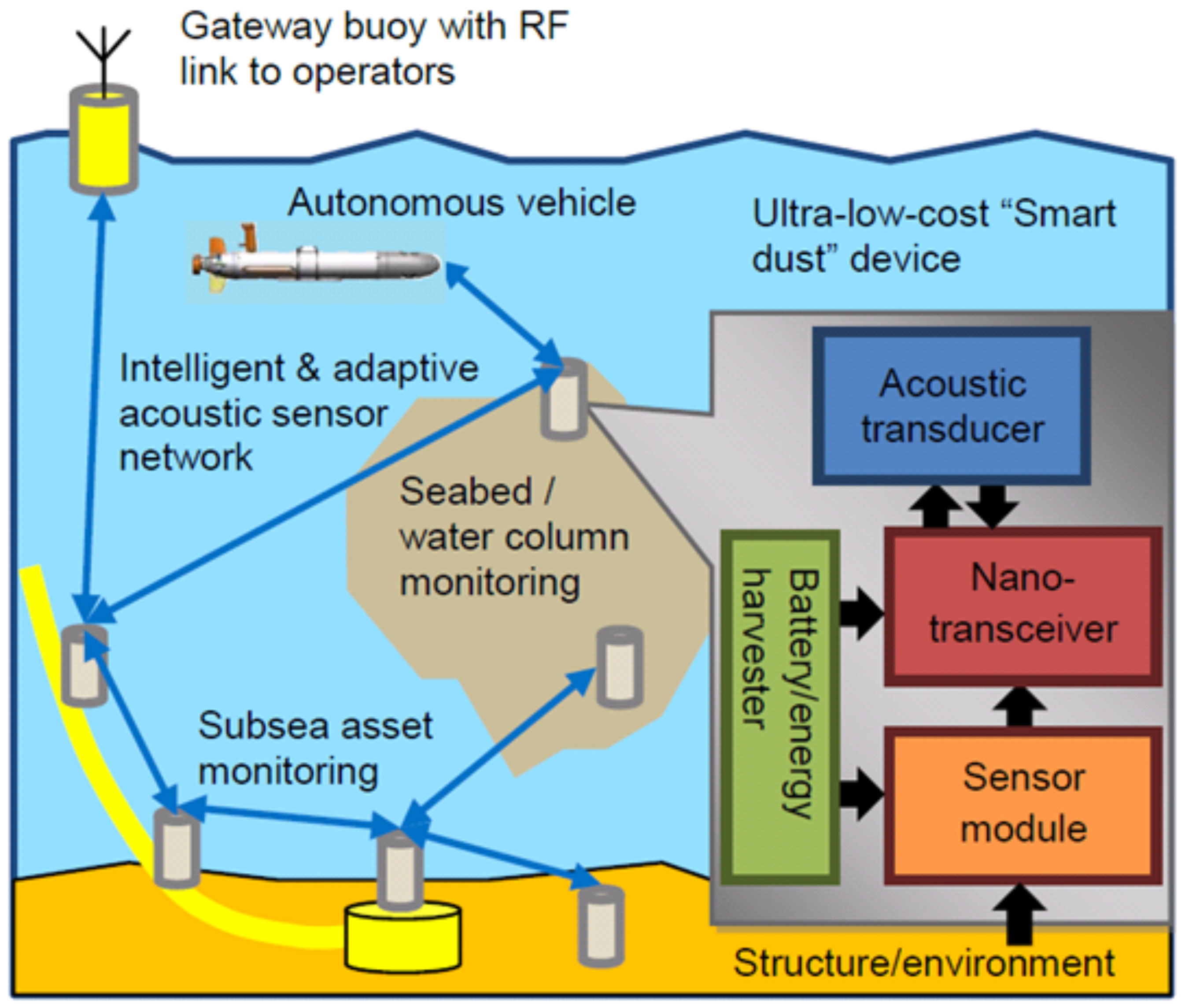
The work presented in this paper is part of the USMART project [25,26,27,28,29]. The aim of the USMART project is to develop affordable technology for large-scale, smart wireless sensing networks. To give context to this research, an illustration of the USMART project as a whole is shown in Figure 4. The illustration shows a network of underwater wireless communication/sensor nodes all linked to a central gateway node with wireless links back to shore.
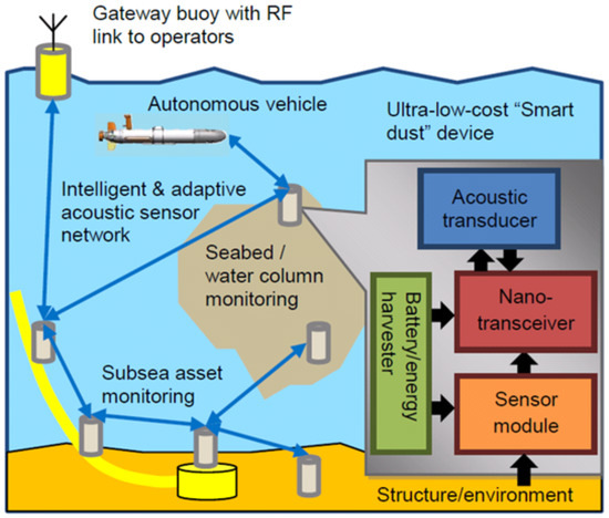
Figure 4.
Project illustration of USMART. The figure shows a wireless underwater network of sensor nodes all linked via acoustic communication to a central gateway buoy. This buoy provides a RF link to relay data back to shore for analysis.
These nodes are able to communicate with the central gateway buoy, as well as relay messages between nodes beyond a single hop, with the aim of expanding the range of the network. The nodes are also able to perform localisation using a combination of underwater acoustic and surface GPS data.
1.4. Project Aims
The aims of this project are as follows:
- Develop passive acoustic vessel detection algorithms that can be implemented with very-low-energy processing (of the order of 10 );
- Compare different approaches with mixtures of analogue and digital processing, and continuous and duty-cycled sampling/processing;
- Adapt an existing low cost/power acoustic modem platform to implement a wireless vessel detection device;
- Demonstrate underwater acoustic transmission of vessel detection information;
- Evaluate system performance in a realistic offshore environment.
2. Methods
As the vessel detector will be integrated with an existing acoustic modem platform, the algorithm design will work with and add to the existing analogue front end of the modem. The acoustic modem is band limited to the propeller cavitation band of interest and resonant frequency of the transducer, which will be used in the remaining vessel detector design.
2.1. Continuous Analogue and Digital Detection (CADD)
The aim of the CADD mode is to implement the DEMON algorithm in a power efficient manner for the purposes of vessel detection. To do this, much of the DEMON method is implemented using carefully designed analogue electronic signal processing circuits. By processing the signal using low-power analogue electronics, the signal can be sampled towards the end of the DEMON process and at a much-reduced sample rate (256 Hz). An illustration of the analogue signal processing is shown in Figure 5, which resembles closely the stages of the basic DEMON structure previously illustrated in Figure 3.
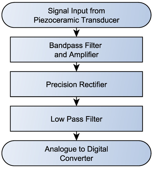
Figure 5.
Flow chart illustrating the analogue signal processing stage of the vessel detector’s CADD mode. The method employed is based on the DEMON algorithm but is implemented using a power efficient analogue circuit design.
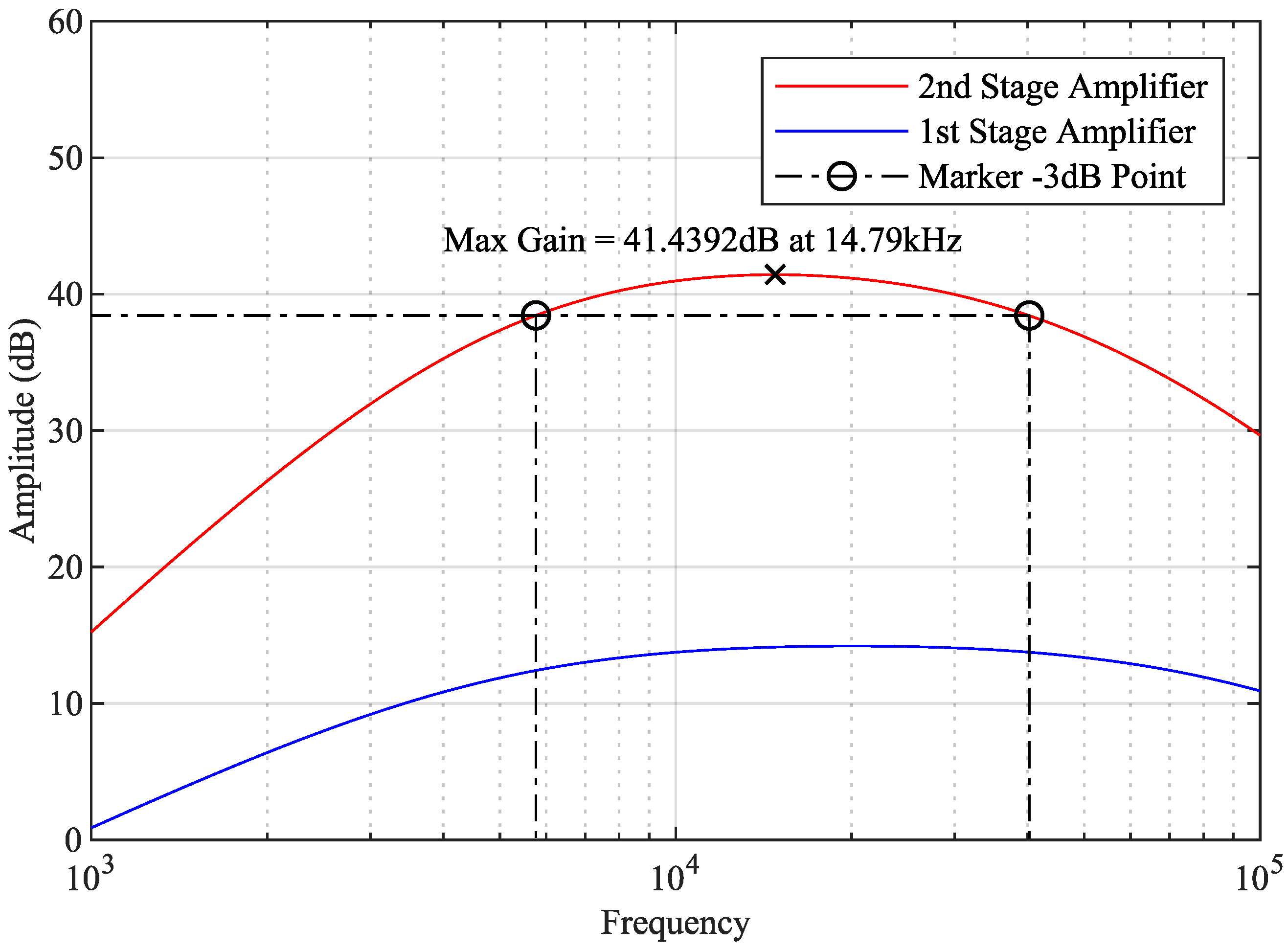
In the first stage of Figure 5, the analogue circuit has been designed to band limit the signal in addition to providing significant amplification. This stage aims to filter out unwanted interference by isolating the typical band of interest for propeller cavitation. This is typically in the 5–40 kHz region, which is also ideally situated for the resonant frequency of the piezoceramic transducer used, which sits around the 30 kHz region. To illustrate the design of this analogue amplifier/filter, Figure 6 shows an LTspice simulation of the analogue circuit. The response shows two stages of amplification, resulting in a total gain of approximately 41 dB for the input signal. The level of gain has been chosen to maximise the performance of the following stage rectifier circuit, in addition to utilising as much of the dynamic range of the ADC as possible. Figure 6 also demonstrates the band pass filtering response of the analogue circuit, with −3 dB cut off points located at 5.7 and 40 kHz, which is ideal for propeller cavitation.

Figure 6.
LTspice simulation results showing the frequency response of the vessel detector’s analogue circuit design.
The final two stages in Figure 5 show an analogue full-wave precision rectifier circuit and a low-pass filter. These two signal processing techniques are used to extract the envelope of the high-frequency, amplitude-modulated input signal. As stated previously, the envelope signal is directly related to the rotational rate of the propeller during cavitation. Capturing the envelope of this high-frequency amplitude-modulated signal, as opposed to the pure high-frequency signal, enables a much lower sample rate.
The remaining stages of the CADD mode all take place in the digital domain. A detailed description of each stage is shown in the list below:
- Sample Rate—The incoming signal is sampled at 256 to capture spectral energy between 0 and 127 . This is the band of interest for propeller cavitation detection using the DEMON method;
- Remove DC Bias—The incoming signal includes a DC bias that is removed by calculating the mean value of the current block of 256 samples and subtracting this value, as shown in (2).
- Data Shift—The microcontroller used is limited to 16-bit arithmetic with a maximum stored number size of 32 bits. In order to preserve the accuracy of data during calculation, binary left shifts are applied to data values prior to calculation being carried out;
- Hanning Window—Before the data is passed to the fixed point FFT (Fast Fourier Transform) routine, it is first windowed to prevent spectral leakage. The Hanning window used has a fixed amplitude of to ensure that there is no chance of binary overflow during the windowing calculation;
- Fixed Point FFT—The KL16Z microcontroller used to implement the detection algorithm uses fixed point arithmetic. Therefore, a fixed point 16-bit FFT algorithm has been designed to work with the hardware available. The main advantage of fixed point arithmetic is the speed at which it can be completed and the minimal strain it puts on the microcontroller. The major disadvantage is the potential loss in accuracy during calculation, as lower resolution bits can be lost due to the limited number size. As implemented prior to the windowing stage, binary shifting is a major part of the FFT routine to preserve accuracy. The fixed point FFT is based on (3) with modifications to enable fixed point arithmetic and maintain data resolution, where , k = index of frequency, n = index of signal, and N = block size.
- FFT Magnitude—The result of the fixed point FFT is a real and imaginary array. Using these arrays, the DEMON magnitude squared is calculated using (4). The reason there is no square root in the magnitude formula is because it would be computationally intensive to complete and it is not required for the end result. As in previous stages, data resolution is maintained by shifting data to maximise the dynamic range available.
- DEMON Spectrum Peak Detection—Now that we have the DEMON spectrum resulting from the FFT, the remaining stages represent the decision-making part of the vessel detection algorithm. The aim is to identify consistent above-threshold spectral peaks in the DEMON spectrum. Therefore, the first task is to identify the peak magnitude and which of the 128 frequency bins it occurs in. Each of these frequency bins represents 1 of resolution. In addition to the largest peak present in the DEMON spectrum, the second largest peak is also identified for the purposes of post processing analysis.
- Magnitude Threshold—The first user defined threshold is related to the magnitude of the DEMON peaks detected. The threshold is currently based on a multiple of the spectrum average. The spectrum average is currently calculated using (5), where X = DEMON spectrum magnitude, n = number of frequency bins, and i = index of signal.Once the peak magnitude threshold has been calculated, it is compared with the detected peak magnitude. If the relationship shown in (6) is not satisfied, with = detected peak magnitude and = calculated magnitude threshold, then a zero value is recorded in the linear fit array to indicate a negative result.
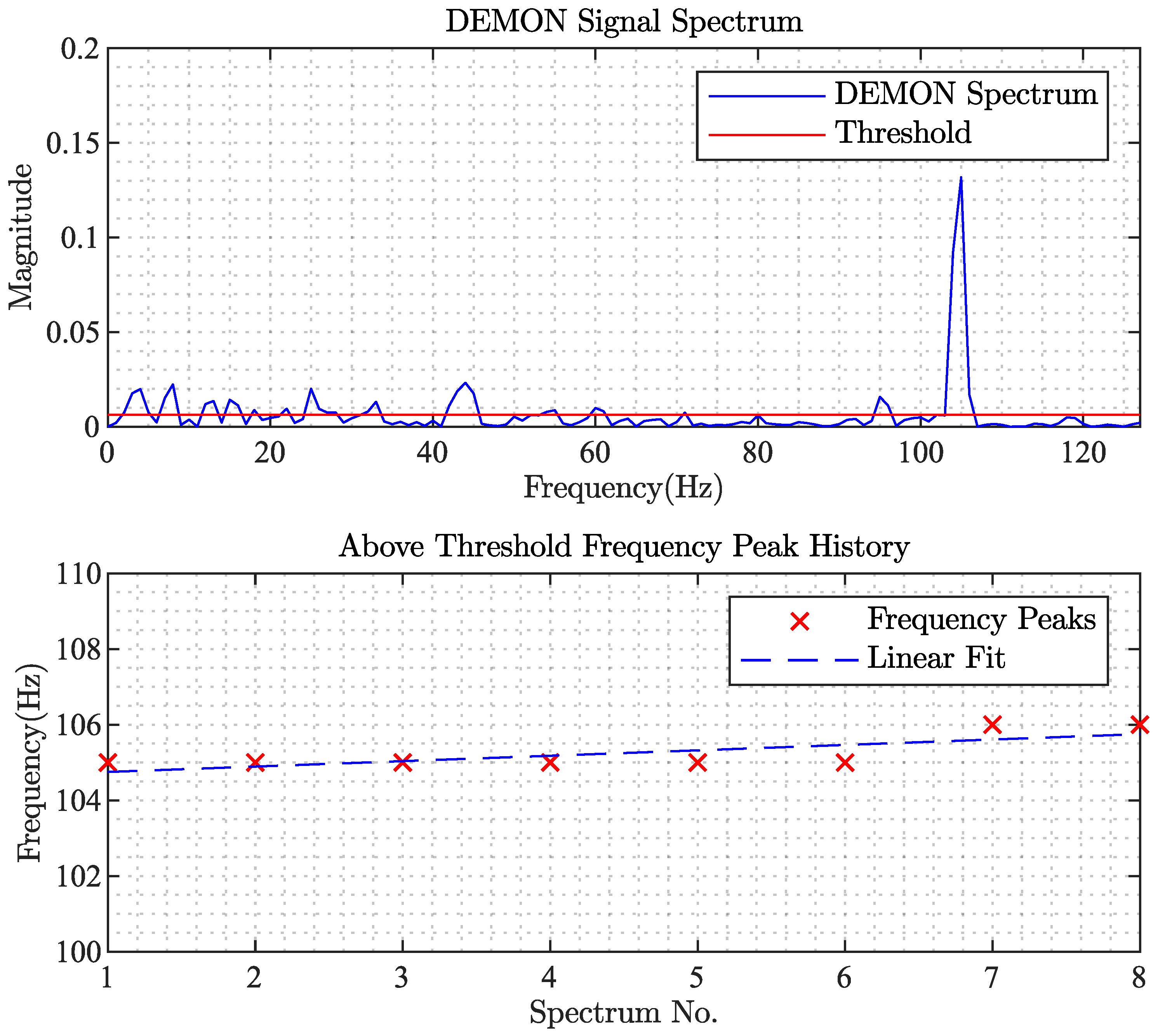
- Linear Fit—As discussed in the previous stage, each time a DEMON spectrum is calculated, the peak magnitude and frequency are recorded for comparison against a user-defined threshold. A line of best fit, represented by , is calculated for the frequency data recorded to establish if a consistent trend exists over time. The formulae used to calculate the line of best fit are shown in (7)–(9).An example of the linear fit applied to frequency data is shown in Figure 7.
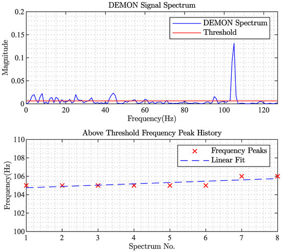 Figure 7. Example of a positive detection spectrum and historical frequency peak record.To quantify the level of trend that exists within the frequency data, a standard error of the estimate calculation is carried out as discussed in the next stage;
 - Standard Error Of the Estimate (SEOE)— To identify if a consistent trend in the DEMON peak record exists over a given timeframe, a line of best fit is applied to the data set and the SEOE (S) is calculated (see Figure 7). The SEOE is a measure of how well the actual recorded samples relate to the line of best fit or estimated samples. The SEOE calculation is shown in (10), where is the estimated samples and y is the actual samples.If the calculated SEOE is below a user defined threshold this would constitute a positive detection as shown in (11).
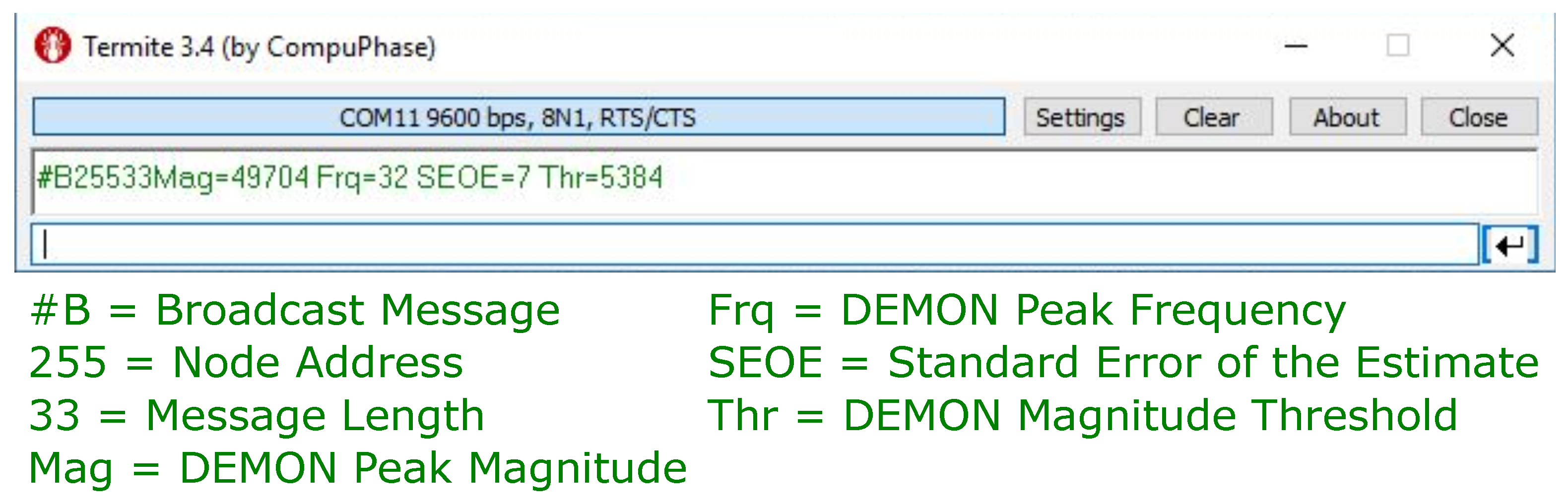
- Detection Decision—Once the previous stages of the vessel detection algorithm have been satisfied, the last part of the process is to package useful data to relay back to the end user. As the vessel detector is integrated with an existing re-purposed acoustic modem, the algorithm simply switches modes to make use of the communication platform. Data is then sent acoustically through the water. An example of the data sent back to shore is illustrated in Figure 8.
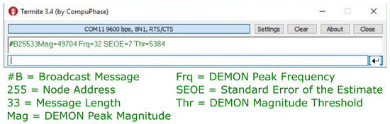 Figure 8. An example of the data packet content, which is sent acoustically through the water to the gateway buoy.
2.2. Non-Continuous (Duty-Cycled) Digital Detection (NCDD)
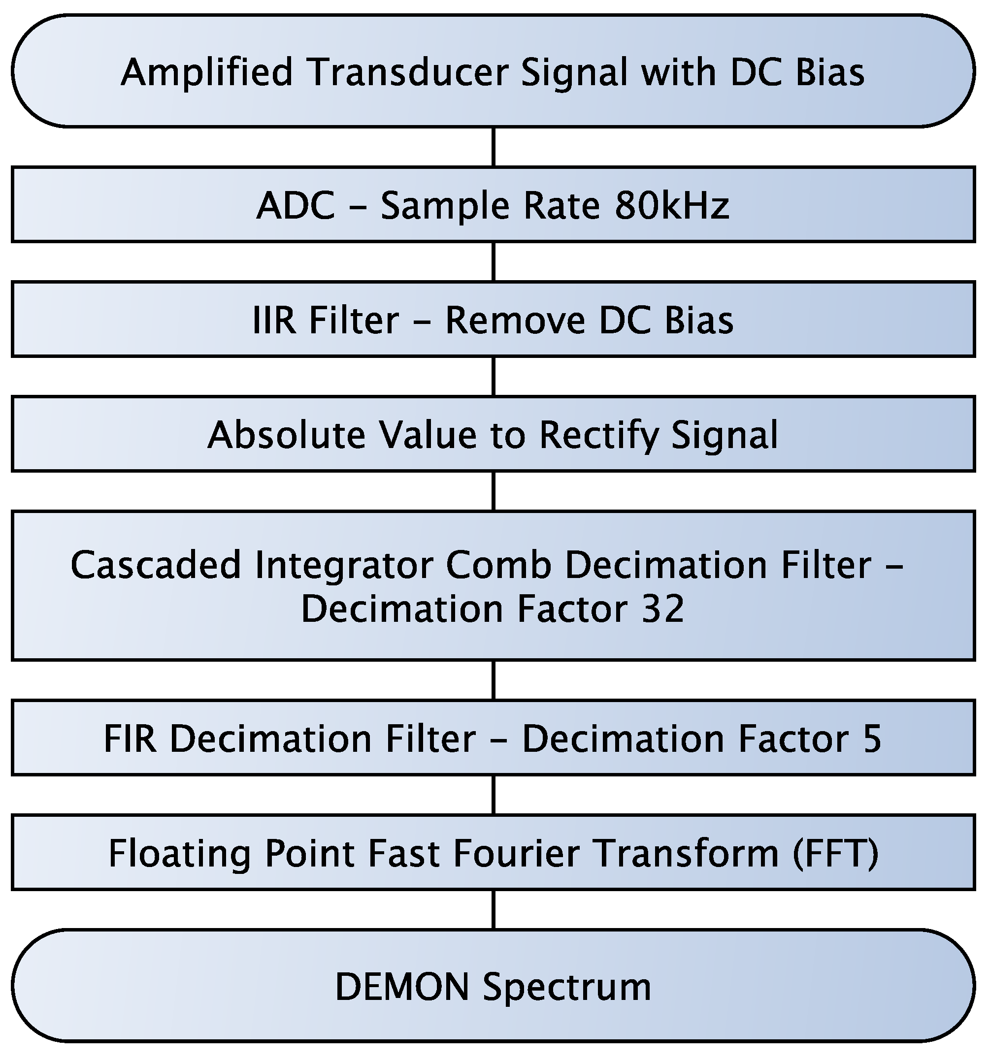
The NCDD mode provides an alternative approach to the previous CADD mode in that the detection process is fully digital and the period of active detection is duty cycled. To make these two modes comparable, the total average power consumption is matched and the overall vessel detection algorithm is not changed. In the NCDD mode, the signal is sampled at 80 , which captures all of the amplified input signal in the 0 to 40 range. High-frequency noise produced during propeller cavitation is typically found in the 5 to 40 kHz range, which satisfies the Nyquist criteria for this mode. The stages of the NCDD mode are illustrated in Figure 9.
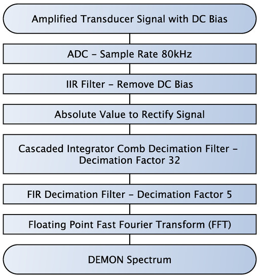
Figure 9.
Illustration of the NCDD mode signal processing method, used to produce the DEMON spectrum. The method combines different digital filtering/decimation techniques in order to maximise processing efficiency and retain spectral resolution.
As shown in Figure 9, the amplified signal is sampled at 80 kHz and the first stage of IIR high-pass filter is used to remove the DC bias added by the analogue amplifier. The reason for this bias is so that the ADC can capture the entire signal, as it is not capable of capturing a negative voltage. Once the signal is sampled, the bias is removed and the absolute value is taken. This is to rectify the signal similar to the analogue precision rectifier in the CADD mode. The next two stages both aim to decimate and low-pass filter the signal to capture the envelope of the now rectifier signal. The reason for starting with a Cascaded Integrator-Comb (CIC) decimation filter is due to the high sample rate of 80 kHz. A CIC filter is a very computationally efficient filter, as it involves only additions and subtractions. The decimation rate is set to 32, which adds to the efficiency, as only one output sample is produced for every 32 input samples. These efficiency measures are at the expense of a less than ideal low-pass filter response. This is illustrated in Figure 10, which shows the filter response of both the CIC filter and the following FIR decimation filter.
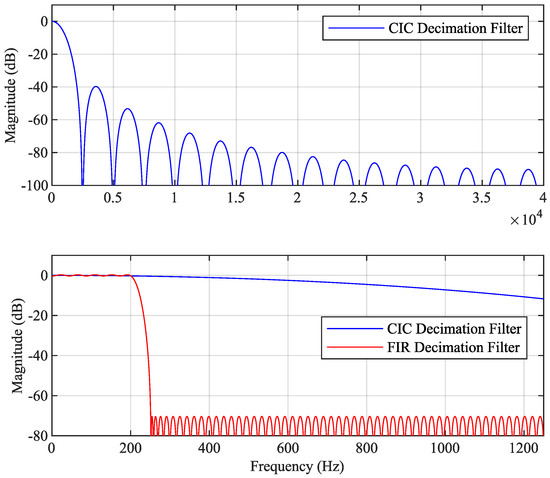
Figure 10.
Filter response of the NCDD mode digital signal processing stage. The plot shows the filter response of a CIC filter followed by an FIR filter, both of which have stages of decimation. The end result is a tightly bound filter response, but the computational load is greatly reduced by using this combination of filters.
The FIR decimation filter is more complex computationally than the CIC filter, as it involves both multiplications and additions. However, this filter runs at 1/32 of the 80 kHz sample rate due to the CIC decimation stage. The FIR filter is set to decimate by a factor of 5 so, including the CIC stage, only one output sample is produced for every 160 input samples. That FIR output signal has now been decimated and low-pass filtered down from 80 kHz to 500 Hz, which preserves spectral content below 250 Hz due to the Nyquist criteria. The final stage in Figure 9 shows a floating point FFT, which calculates the spectral content of the signal.
One of the key features of the NCDD mode is the improved precision gained by using a floating point FFT to produce the DEMON spectrum. This improved precision can be a great advantage in detecting very small signals from distant vessels.
2.3. Data Transfer
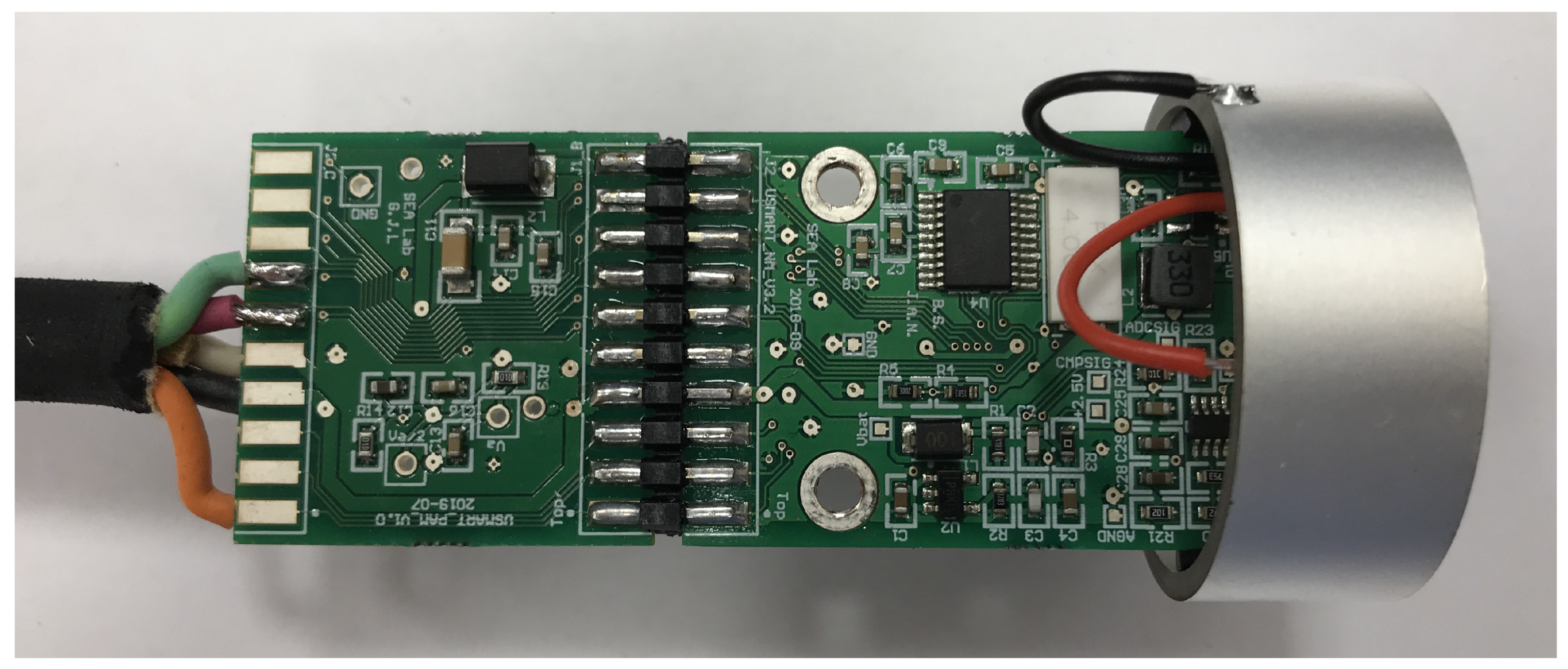
Data communication is enabled using a low-power, low-cost acoustic modem, which is capable of sending data through the water reliably a distance of up to 2 km in a single hop. Further details on the features and functionally are detailed in the authors’ prior paper [16]. Figure 11 shows the communication device PCB (larger right-hand PCB) along with the vessel detector’s analogue signal processing PCB (smaller left-hand PCB). The shared piezoceramic transducer, which performs both sensing and communication tasks, is also shown.
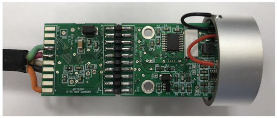
Figure 11.
Completed assembly of vessel detector and communication device prior to encapsulation. The smaller left-hand PCB houses the analogue circuit used in the CADD mode. The larger right-hand PCB belongs to the communication device. The on-board microcontroller and transducer crystal are shared for both communication and vessel detection tasks.
2.4. Enclosure
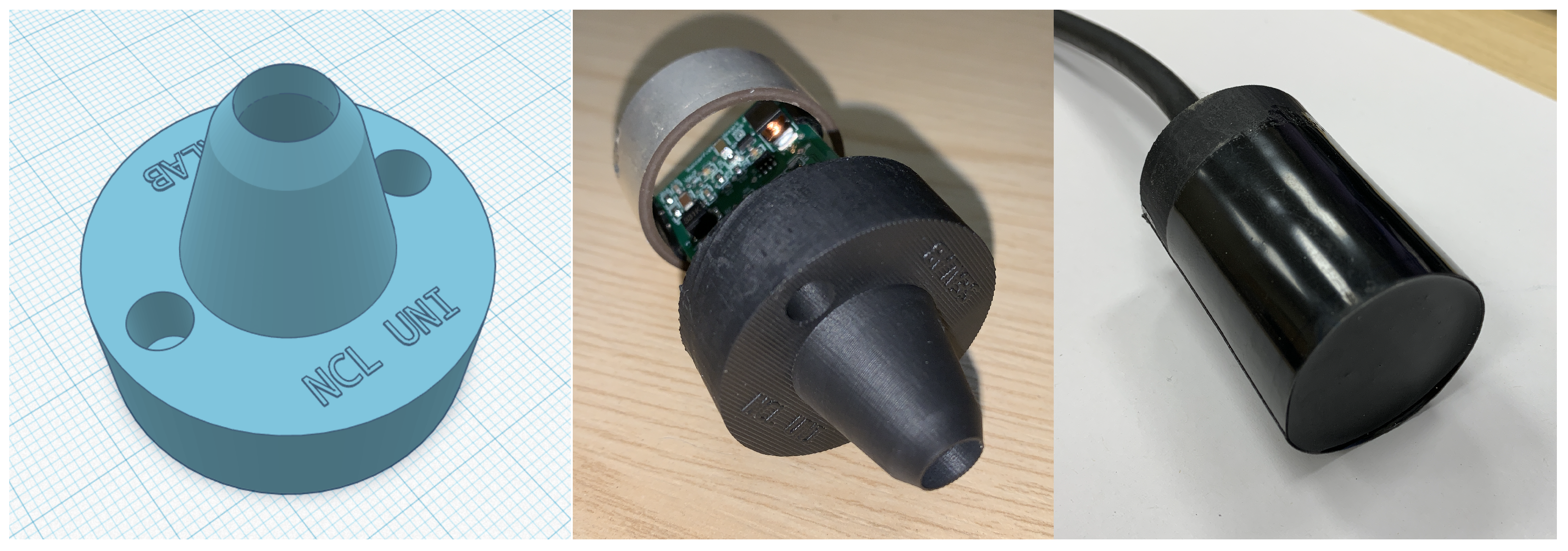
The vessel detector enclosure must be designed to enable a deployment duration of up to one year at a minimum depth of twenty metres. In addition, the enclosure must be low-cost to enable the unit to be scaled to achieve the USMART project’s aim of developing an affordable underwater wireless network. Although this project is still in the proof-of-concept phase, considerable thought has gone into designing a low-cost reliable enclosure that is easily scalable. To do this, off-the-shelf components have been used wherever possible and any custom processes have been designed with portability to full-scale manufacturing in mind. Figure 12 shows an example of a bespoke 3D component created to aid the encapsulation process of the detector PCB and transducer. The 3D component also includes a cable gland and mounting holes in anticipation of producing nodes on a large scale.
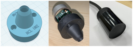
Figure 12.
This figure shows the design and construction of a 3D printer encapsulation component. This shows progress made to enable mass production of the potted vessel detector/communication device. Key design aspects in the 3D printed design include: cable gland, mounting holes, PCB holder, and transducer end potting process.
2.5. Experiment Location and Setup
A key enabler for the near-real-time collection of vessel detection data is an off-shore gateway buoy. Designed and commissioned by Newcastle University’s SEA Lab, the gateway buoy is complete with a dedicated WiFi link back to the campus network. The gateway buoy is equipped with two hydrophones sampling at 96 kHz, which is streamed in near real time back to shore for secure storage on the university network. The buoy also contains two of the acoustic modems on which the vessel detector hardware is based. This dual-redundancy receiver system allows for reliable collection of vessel detection data over long periods of time. The buoy is powered using external solar panels that charge internal battery packs. Figure 13 shows how the gateway buoy is located in relation to the vessel detector’s moored deployment.
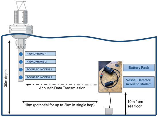
Figure 13.
Diagram of the North Sea experimental deployment. The central gateway buoy provides a link back to the university campus network. This affords near-real-time data from the vessel detector, which is located 1 km away from the buoy at a depth of 20 m from the surface.
The gateway buoy highlighted in Figure 13 is positioned at a distance of 1 from the deployed node. This was to ensure that acoustic communication performance was not an influencing factor in the detection results. The trials are designed to test the vessel detector’s performance in successfully identifying vessels using passive acoustics. The acoustic communication is included to show the vessel detector as a complete system ready for practical use cases.
3. Results
3.1. Initial Validation Experiment
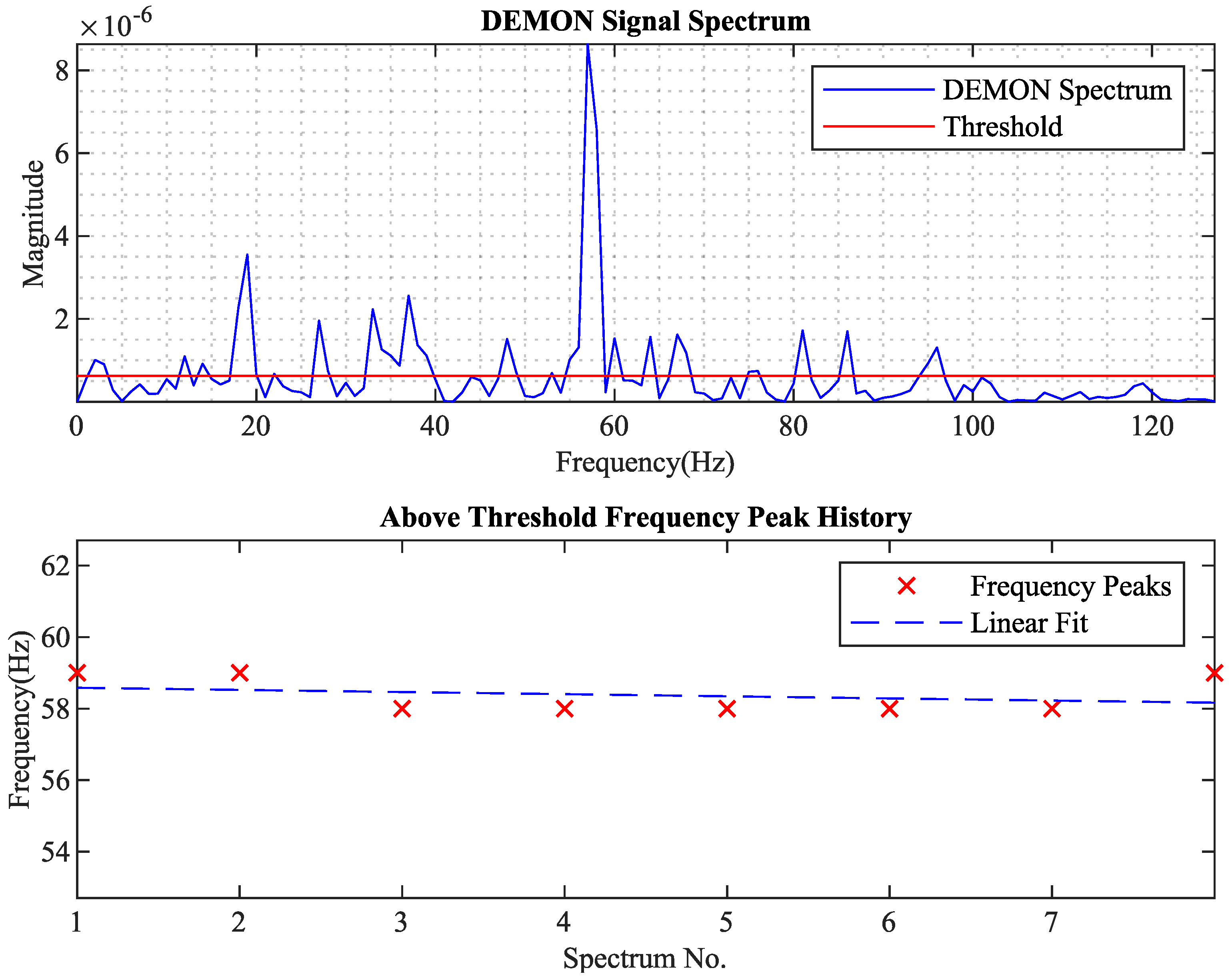
In this controlled experiment, a RHIB owned by Newcastle University was instructed to make several passes near to the vessel detector within the Port of Blyth estuary. The vessel detector, setup in CADD mode, was deployed directly from a jetty and results were monitored using a connected laptop in real time. The aim of this experiment was to validate that the vessel detector is capable of passively detecting the RHIB based solely on the signal created during propeller cavitation. Figure 14 shows one of the positive detections achieved while monitoring the RHIB in a controlled estuary environment. The two largest peaks in the DEMON spectrum can be found at 19 and 57 Hz.
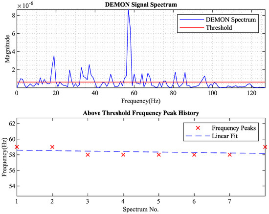
Figure 14.
Data produced by the vessel detector while monitoring the passing of a RHIB. The plot shows DEMON spectrum data during a positive detection along with historical peak frequency data. The historical peak frequency data has a linear fit applied, which is part of the low-power detection algorithm.
Pollara et al. showed that DEMON spectrum peaks are related to the rate of rotation of the propeller shaft and the blade rate [30]. Using these two spectral peaks, it is possible to calculate the number of blades on the vessel itself. This information may be useful when it comes to classifying a vessel type. The relationship used to calculate the number of blades is shown in (12).
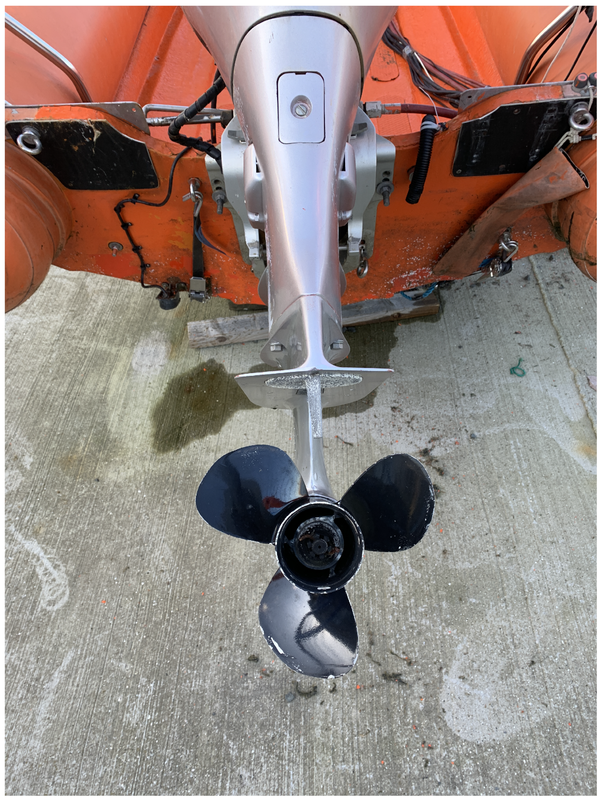
Using the DEMON peaks in Figure 14, the number of blades calculated was shown to be three. This is verified to be a valid calculation by Figure 15, which shows that there are indeed three blades on the recorded RHIB.

Figure 15.
Photo of the detected RHIB showing the number of blades on its propeller.
This experiment demonstrates the system’s ability to passively detect a key target vessel type (small RHIB) using passive acoustic monitoring. It also shows that the data produced during detection can offer more information about the vessel, such as number of propeller blades.
3.2. Open Sea Trials
In this experiment, the vessel detector was deployed in open sea at around 3 from the Blyth, Northumberland coastline. The detector, setup in CADD mode, was completely isolated on a mooring and used acoustic communication to relay data via a WiFi-enabled gateway buoy, as described in Section 2.5. The aim of the open sea trial was to test the system’s ability to detect vessels in open sea and successfully relay this data back to shore. The isolated mooring was meant to mimic the potential end user deployment as much as possible and test the equipment against the harsh North Sea conditions. Open sea offers a new dynamic where there is no control over the number of vessels present at any one time. These single- and multi-vessel scenarios are reflected in the two sub-sections of results for this trial.
3.2.1. Single Vessel Results
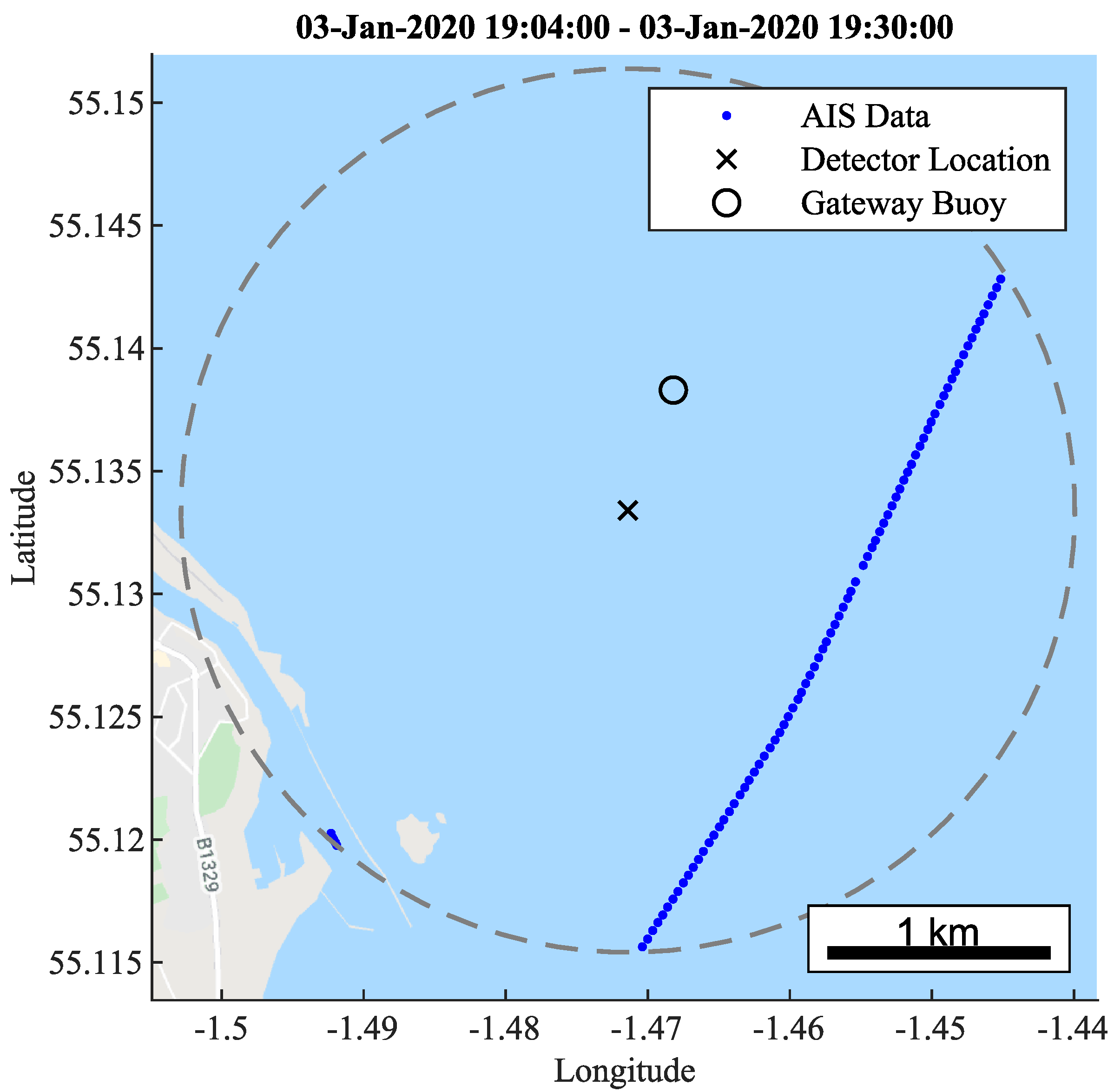
An example of a positively detected vessel achieved during the open sea trial is shown in Figure 16 and Figure 17. Figure 17 shows a time stamp comparison of vessel detection data and local AIS data (within 2 km of detector) to illustrate any overlaps of data points in time. These overlaps represent a true positive detection result, as both the vessel detector and local AIS data agree that a vessel was present at that point in time. The 2 km radius for AIS data was chosen, as this represents a distance where the vessel detector is expected to perform well. Moreover, from a wireless network point of view, a 2 km distance between nodes would be within the communication device’s acoustic range capabilities.

Figure 16.
AIS positional data of the detection plotted over a map of the deployment location [31]. The map illustrates the AIS location of the vessel as well as the detector and central gateway buoy. The dashed circle represents a 2 km detection radius around the vessel detector’s location.
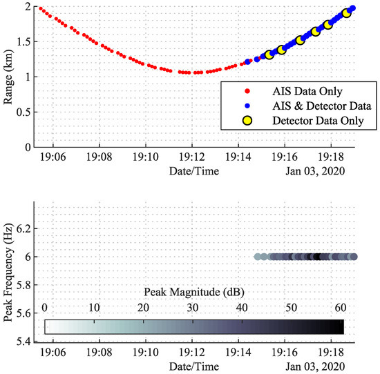
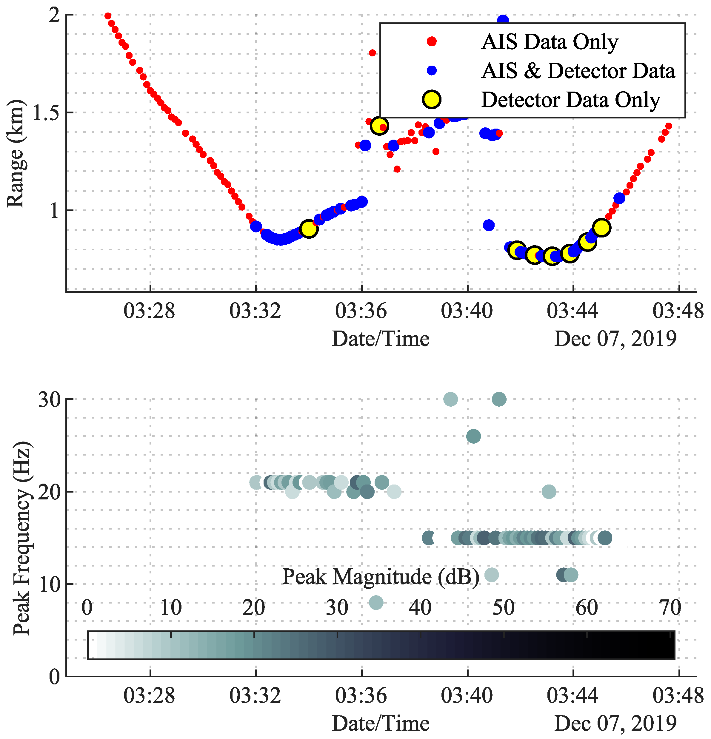
Figure 17.
Illustration of a fishing vessel detected by comparing detection time stamps with local AIS data. The first plot shows the DEMON detection data plotted against range provided by the AIS data. The second plot shows the peak frequency and magnitude detected during this period.
The results do show that there are occasions where AIS data and detection data do not align in time, which is illustrated by the yellow markers. However, it is clear that these are true detections, as the vessel could not have left the area and returned so quickly.
Figure 17 also highlights a detection issue related to vessel orientation relative to the sensing node. A rear-powered vessel will radiate cavitation noise more intensely in the direction away from the rear of the vessel. This is due to the obstruction of the vessel itself in the forward propagation path. This results in vessel detections occurring once the vessel is orientated so that the propeller faces in the direction of the sensing node. This is illustrated in Figure 17, as the vessel was detected after the minimum range was reached at around 1 . After this point in time, the range was increasing, which indicates that the vessel was moving away from the sensing node; subsequently, positive detections begin to be recorded.
3.2.2. Multi-Vessel Results
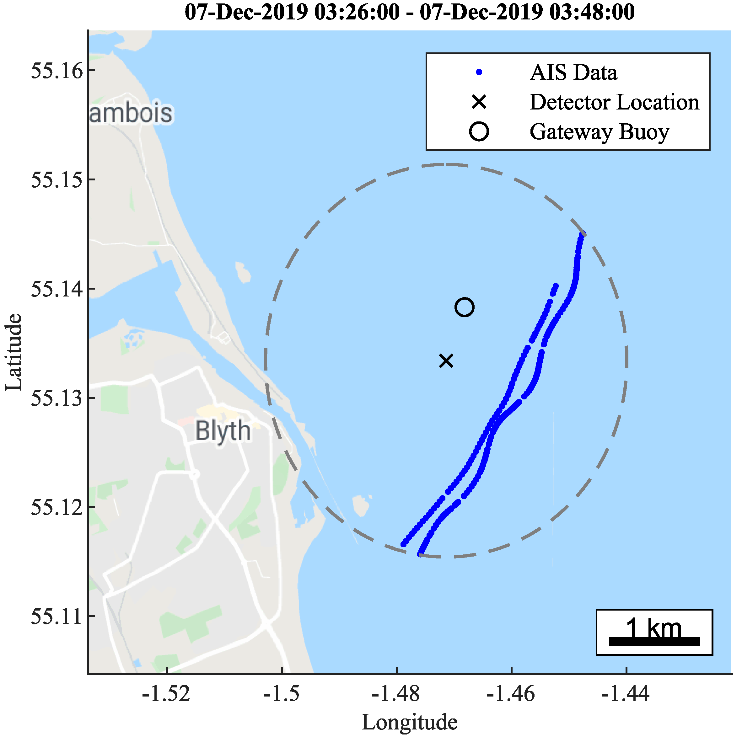
During field trials, there were numerous occasions where multiple vessels were present at a similar range within quick succession. An example of this is shown in Figure 18 and Figure 19. Using the DEMON spectrum detection data provided by the vessel detector, it is possible to make a distinction between these two closely linked events. The peak frequency detected during this time shows two distinctive trends, with a notable step change at approximately 03:38.
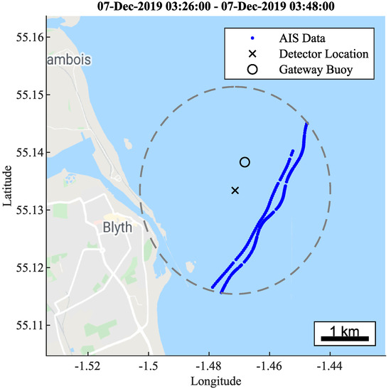
Figure 18.
A map of the AIS location data confirms that two vessels were present during the detection time window [31].

Figure 19.
Illustration of two vessels detected within close succession. The first plot shows detection data compared with local AIS data. The second plot shows the DEMON peak frequency and magnitude detected during this period, and a clear step change in frequency is observed.
The first peak frequency trend falls around 21 Hz which is then followed by a sudden step change to 15 Hz. This could simply be a change in speed by a sole vessel; however, when the detected magnitude data is also analysed, it suggests that two different vessels may be present. When a vessel passes a single monitoring point, the magnitude of the cavitation noise would be expected to follow a low-high-low trend over time. This pattern is shown in the magnitude data in Figure 19, which is represented by shading, going from light-dark-light over time. As this pattern happens separately for each of the detected frequency patterns, it suggests that this is indeed two separate vessels passing the same point of monitoring at a similar distance. This is further validated by AIS positional data, which is used in Figure 19 to calculate the distance between the vessel detector and surrounding vessels.
In summary, this field trial demonstrated the vessel detector operating in isolation in an open sea environment. The results showed that the detector has the ability to detect a single vessel, with local AIS data to reinforce the detection result. The results have also demonstrated how the vessel detector can be used to distinguish between two vessels, relying solely on the data provided by the vessel detector.
3.3. Reliability
The reliability of the vessel detector was measured in two areas: noise rejection and detection accuracy. In this experiment, vessel detector data from a long-term field trial (2016 h of monitoring) was analysed to evaluate each of the reliability areas. During this long-term experiment, the vessel detector was operating in its CADD mode.
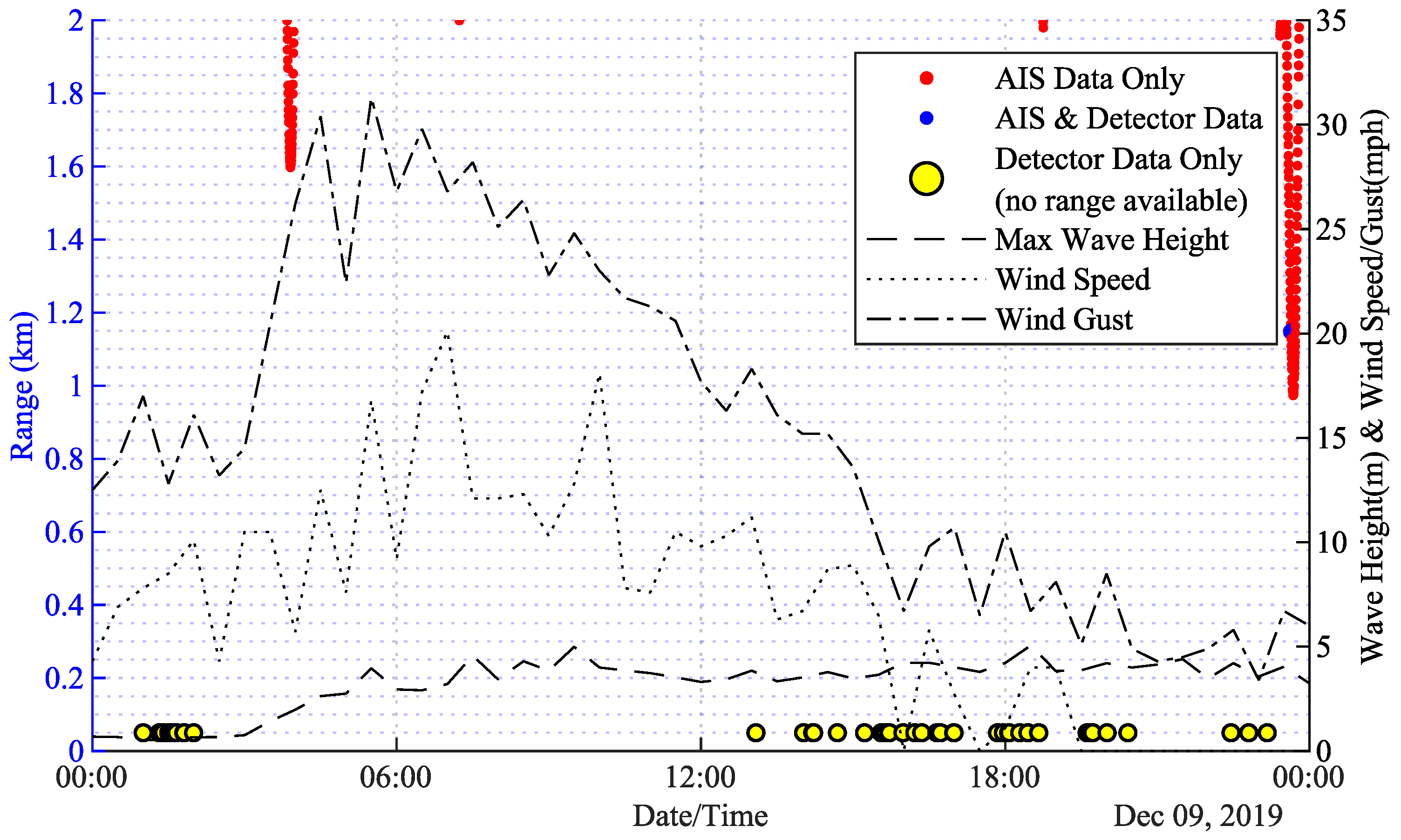
3.3.1. Noise Rejection
The first reliability area is related to severe weather conditions experienced during field trials and how the detector performs under these periods of elevated background noise. Figure 20 shows a 24 h period where no vessels were detected for a substantial percentage of the day. During this period, the weather conditions were very poor, as illustrated by the wave and wind data in Figure 20 [32]. During the period between 06:00 and 12:00, the weather was at its most extreme and no detections were produced. This could indicate that during poor periods of weather where interfering noise is likely to be elevated, the vessel detector remains robust against producing false detections due to interfering noise. This is extremely important from a reliability point of view, but also from power efficiency perspective, as false detections would drain the battery and shorten the deployment duration. Another possibility is that the detection data simply did not make it back to the gateway buoy; however, using the data sequence identifier in the data payload, this was ruled out. Local AIS data indicates that the results received by the vessel detector during this period of poor weather were accurate, as no vessels were reported to be within detection range at the time. However, it must be noted that there is no legal obligation for certain vessels to carry an AIS transmitter; therefore, an absolute ground truth is very difficult to establish for this field trial.
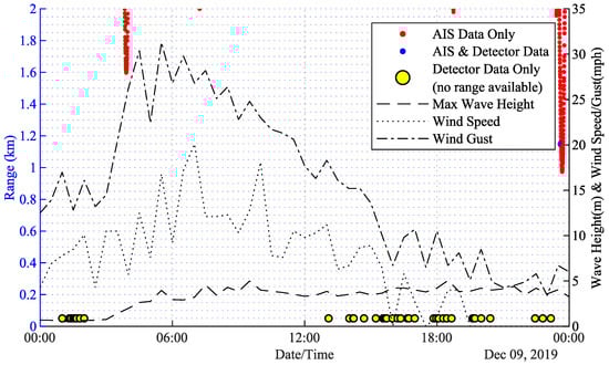
Figure 20.
An illustration of the vessel detector operating in adverse weather conditions. The plot shows AIS and detection data plotted alongside meteorological data [32].
3.3.2. Detection Accuracy
The second reliability area relates to detection accuracy, which compares local AIS data with detection data to evaluate reliability. The following list illustrates each of the four possible outcomes when comparing local AIS data (within a 2 km radius of the vessel detector deployment location) against detection results data. As previously stated, there is no legal obligation for all vessel types to carry or use an AIS transmitter. However, for this field experiment, the local AIS data will be used as the best ground truth available against which to compare the detection data.
- True Positive [TP]—Vessel detector data matches local AIS data (within 2 km radius of detector) during the same one-minute interval;
- False Positive [FP]—Only vessel detector data present within a one-minute interval;
- False Negative [FN]—AIS data detected within a 2 km radius of the detector, but no vessel detector data received within the same one-minute interval;
- True Negative [TN]—No AIS data or vessel detector received during a one-minute interval within the 2 km detection radius.
Results are obtained by examining each one-minute interval of the entire 84-day data set. In each of these one-minute intervals, there are four possible outcomes. Figure 21 shows each of the outcomes as a percentage for the entire 84 days of data collected. The true negative category implies that no vessels are within the detection area, and as expected, this constitutes the majority of the 2016 h of monitoring, with 94%. This is an incredibly important result, especially from a power efficiency perspective, as it shows that for the majority of time, the detector is monitoring, but not transmitting data when it is not necessary to do so.
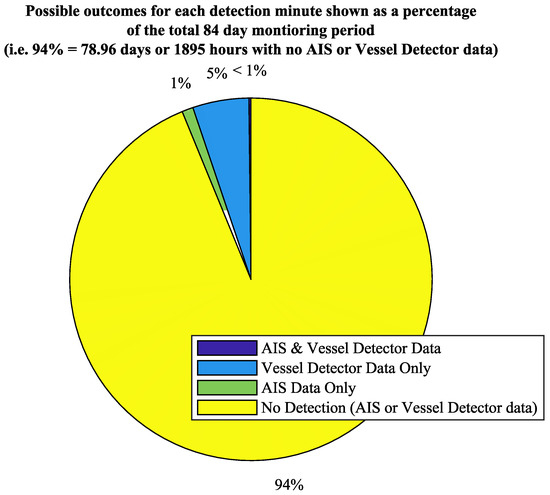
Figure 21.
Detection results gathered from 84 days of deployment. The results are based on comparing local AIS data with the vessel detector data within a detection radius of 2 km. The chart shows the percentage for each of the four possible outcomes for the 84 days data set.
The next most frequent outcome is false positive at 5%, which covers detections which do not have corroborating AIS data within the same one-minute interval. This is a difficult category, as there is no way of knowing for sure how many of these results are due to a vessel simply not having an AIS transmitter and how many are genuine falsely-triggered detections. Again, for the purposes of providing a measure of reliability, AIS data is considered the best available ground truth and the reliability results work on this assumption.
The next outcome is false negative, in which is when there is AIS data within the detection radius, but the vessel detector does not detect anything at the time. This makes up only 1% of the monitoring time during the experiment and could be due to many reasons, including distance, signal strength, vessel orientation, sea conditions, vessel type (i.e., sail boat), and vessel engine status (i.e., could be idle). A vessel’s orientation relative to the sensing node has already been illustrated as a detection issue by field trial results presented in Section 3.2.1. Another potential reason for the false negative result is that the vessel detection algorithm may require further threshold refinements. However, given that this result constitutes only 1% of 84 days of monitoring, it is an encouraging initial open sea deployment result and shows the high detection rate of vessels within 2 km.
The final outcome is true positive, which represents the times when both the vessel detector and local AIS data agree that a vessel is present within the 2 km detection area.
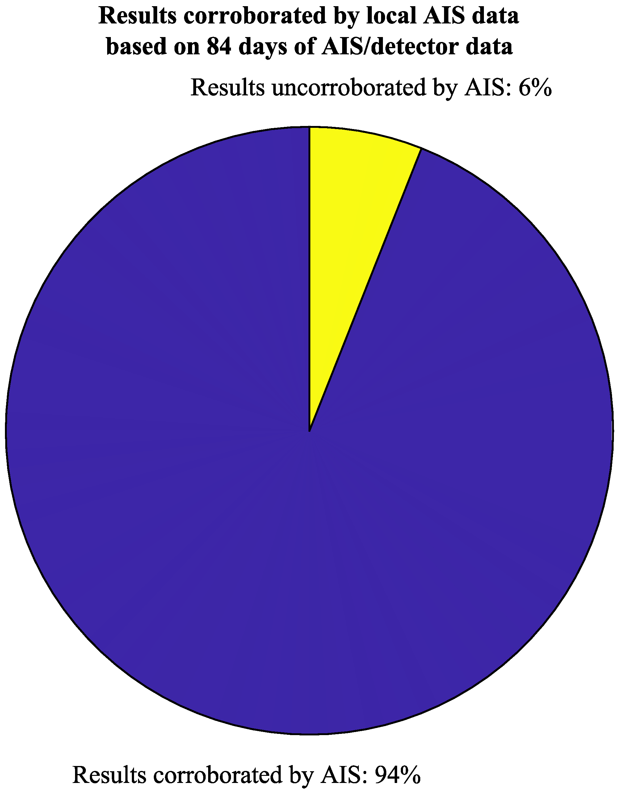
Using the data for the four possible outcomes, Figure 22 shows the percentage of results that were corroborated by local AIS data. This shows that 94% of the results produced were verified using the best available ground truth.

Figure 22.
Percentage of results that were corroborated by local AIS data.
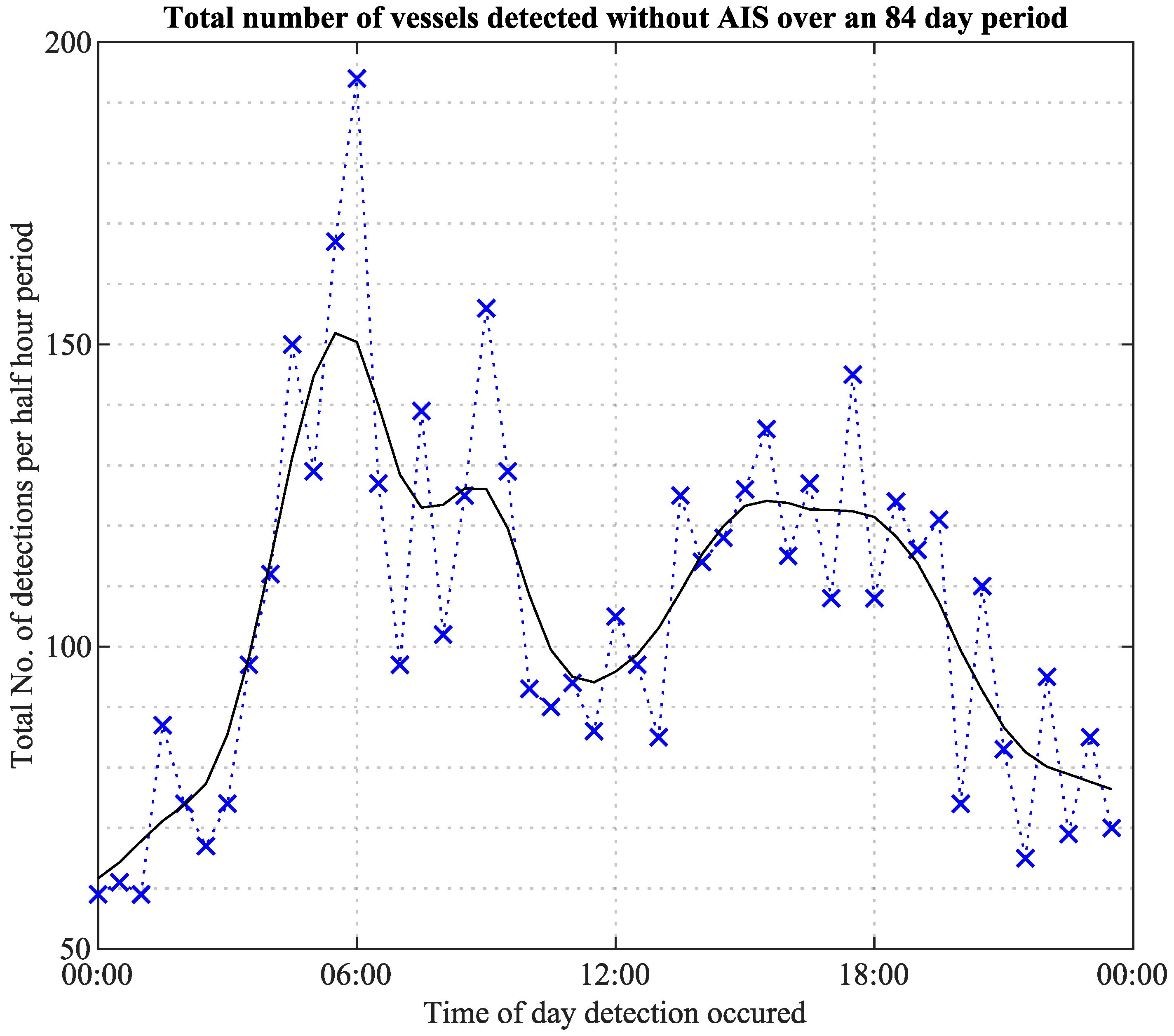
As the results in Figure 21 show, there are many detections where no AIS data was present during the same one-minute time interval. These results have so far been classified as false positives for the purposes of analysing reliability in the absence of a true ground truth. We know that this classification is not completely true, as there is no legal requirement for certain vessels to carry AIS transmitters; therefore, a vessel may be present that has no AIS system on board. Many small vessels in the local fishing fleet or leisure users do not carry AIS. The only way that a 100% accurate ground truth could be obtained is by 24 h visual survey, which is not practical. Figure 23 illustrates the detection data where no AIS was present for various times of day. The plot was created using the total number of non-AIS detections for half-hour intervals using the entire 84 days of data.
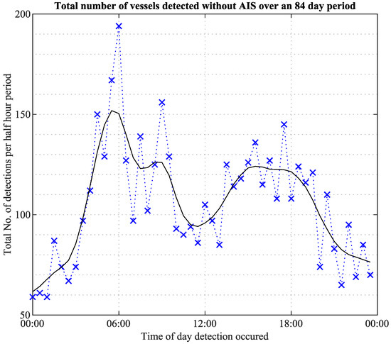
Figure 23.
The total number of vessels detected with no corresponding AIS over a 24 h period using 84 days’ worth of data.
The black trend line in Figure 23 contains dominating peaks, one in the early morning (06:00) and another in late evening (17:30). This may correspond with fishing traffic leaving Blyth Port at first light and then returning in evening before sunset. The data also suggests a higher-than-expected average of around 100 total detections per half-hour period using the entire 84 days of data. Many of these may be duplicate detections of the same vessel within a half-hour period. Without AIS data, it is difficult to say whether this average is accurate or whether there are some false detections within the non-AIS detection data.
To summarise, the reliability results presented are based on a long-term deployment of the vessel detector in harsh North Sea conditions. The detector was shown to operate in CADD mode during periods of intense weather. This shows that the algorithm is unlikely to produce false detections due to weather-related noise. Detection accuracy is an important factor, as any end user wants to have confidence in the detection data produced. In this trial, 94% of results were able to be corroborated with the best available ground truth, which is local AIS data.
3.4. Deployment
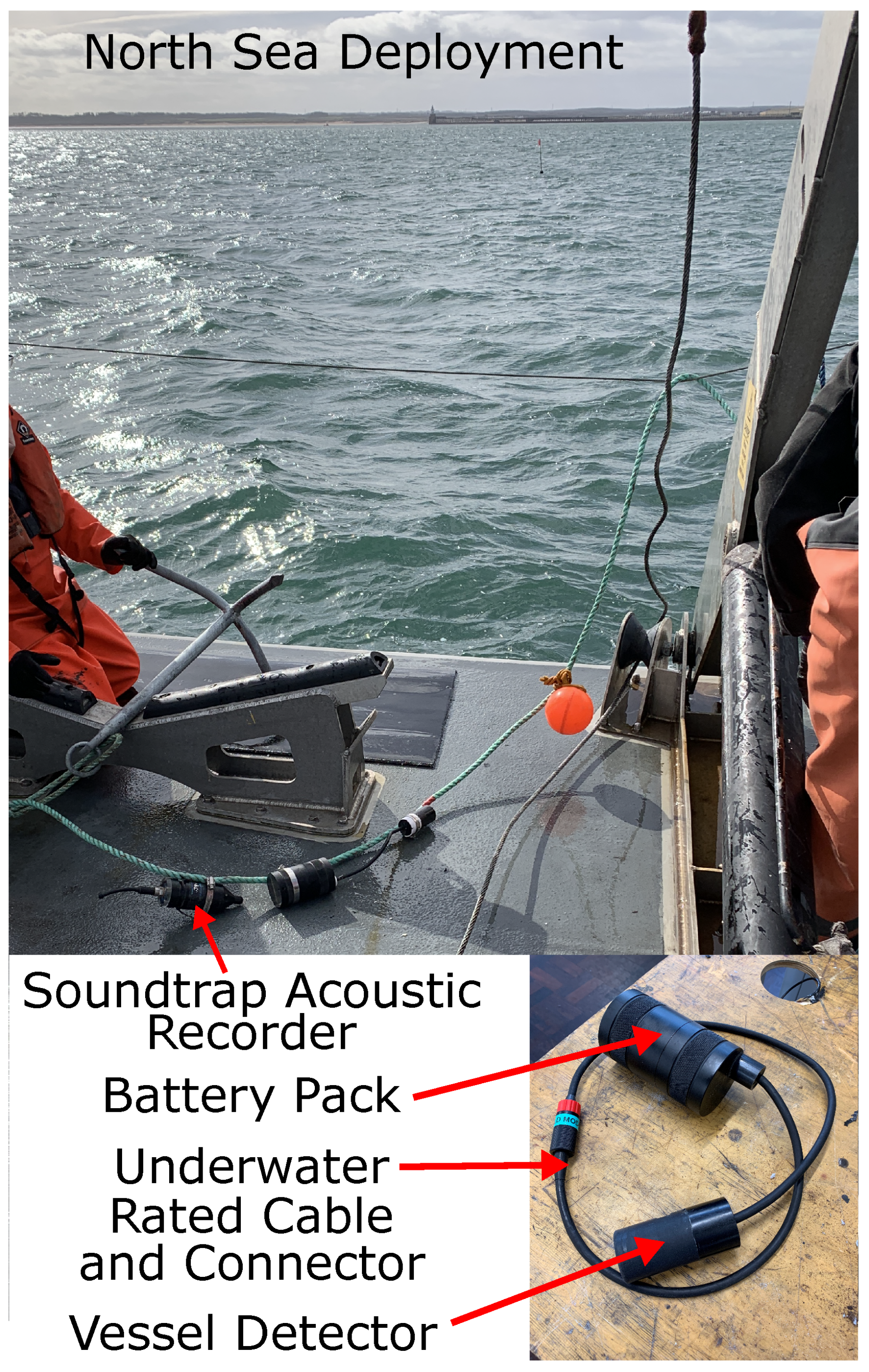
The latest deployment of the vessel detector is shown in Figure 24. The deployment rig shows the detector and battery pack accompanied by a Soundtrap device used to aid algorithm development in post-processing. The Soundtrap is a commercially available underwater recording device capable of sampling data at a rate of up to 576 kHz and storing this data using on-board memory [33].
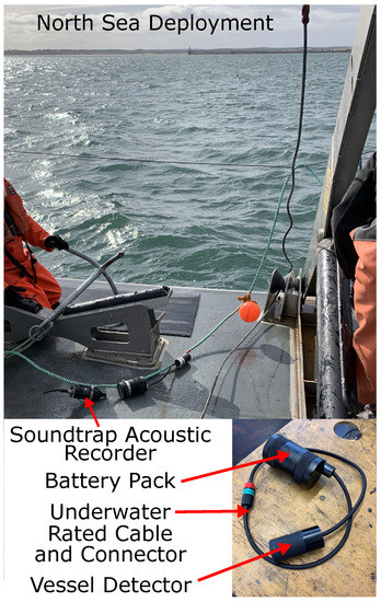
Figure 24.
Photo of the vessel detector being deployed in the North Sea. The deployment line contains the vessel detector with battery pack and also a Soundtrap recorder [33].
To maximise the deployment duration, the power efficiency of the vessel detector is paramount. Some of the initial power saving methods adopted in the vessel detector’s design are documented in previously published research by Lowes et al. [16]. Further refinements have now been made and the vessel detector has been subjected to a long-term deployment where power efficiency can be evaluated.
During initial validation field trials, there was no restriction on how often the vessel detector could send data when a vessel was detected. One of the modifications made for the long-term field trial was to limit this potential continuous stream of data for the same vessel; the main reason being that acoustic transmissions consume significantly higher power (∼1.5 W) than the detection system. To limit unnecessary transmissions, the detector was programmed to only transmit a positive detection every minute unless the peak frequency detected was notably different from the previous detection. The reason for this is that if two vessels pass within the same time period, then the detector should ignore the one-minute limit restriction and report data unrestricted. This rule is based on the peak frequencies being different during the time period in which the two vessels pass. As shown in Section 1.1, the peak frequency of a vessel’s DEMON spectrum is directly related to the rate of rotation of the vessel’s propeller.
Given that the vessel detector is an event-driven system, the total deployment life will depend on the number of data transmissions. Current field trials achieved 84 days of verified functionality. Deployments of less than one month would not provide enough variability in weather conditions and vessel types to effectively evaluate the system. Using the average power consumption while detecting (11.4 mW) along with the battery pack power capacity (46.8 Wh), an estimated deployment duration of 4–6 months would be reasonable.
3.5. Retrieval
The vessel detector was deployed twenty metres below the surface in complete isolation. The ability to safely retrieve the device is important both from a cost point of view and from an environmental aspect. The oceans are already under severe threat from plastics pollution and this project certainly does not want to add to this problem. Two modes of operation were specifically designed to aid in the retrieval and condition monitoring of the vessel detector when deployed. The first is a ‘ping mode’, which utilises the integrated communication device’s ability to give a point-to-point range measurement using acoustic propagation time. This enables a retrieval vessel to triangulate the position of the detector using periodic ‘ping mode’ range measurements. The second mode is an ‘I’m alive’ routine, which transmits a message acoustically through the water every six hours. This message contains some diagnostics data, including the current on-board battery voltage; however, its main function is to periodically check in to confirm that the unit is still operational. This is important, as the detector is an event-driven device, so without this mode the detector would only contact the shore if and when a vessel passes its location.
3.6. Data Transfer
The vessel detector makes use of a communication device to send data acoustically through the water. There are two messages that the detector may send depending on which mode the device is in at the time. The first message type relates to a vessel being detected and the second message is a periodic diagnostic message used for condition monitoring. Both of these message types contain a selection of the following items within the message payload.
- Message ID—Used to distinguish itself from other deployments using the same communication technology;
- Node Address—A unique address specific to a single node;
- Sequence—An on-board message sequence number used to identify missed data on the receiver end;
- Magnitude—Contains the magnitude data from the on-board FFT calculation for both the first and second largest peak;
- Frequency—Contains the frequency bin to which the first and second largest peak relate to in the calculated FFT;
- SEOE—A measure of how well the calculated frequency samples relate to a line of best fit using SEOE;
- Threshold—The magnitude threshold at the time of detection;
- Battery Voltage—A measure of the current battery voltage on the attached battery pack.
A ‘vessel detected’ message contains all of the items listed, but the data is compressed to take up only 24 bytes to maximise efficiency. This data is sent through the water; using a data acknowledgement feature of the communication device, it is possible to confirm its delivery. Should this acknowledgement not arrive back at the vessel detector, the algorithm has been designed to re-transmit data for a specified number of attempts before the message is abandoned.
3.7. Non-Continuous Digital Detection (NCDD) Analysis
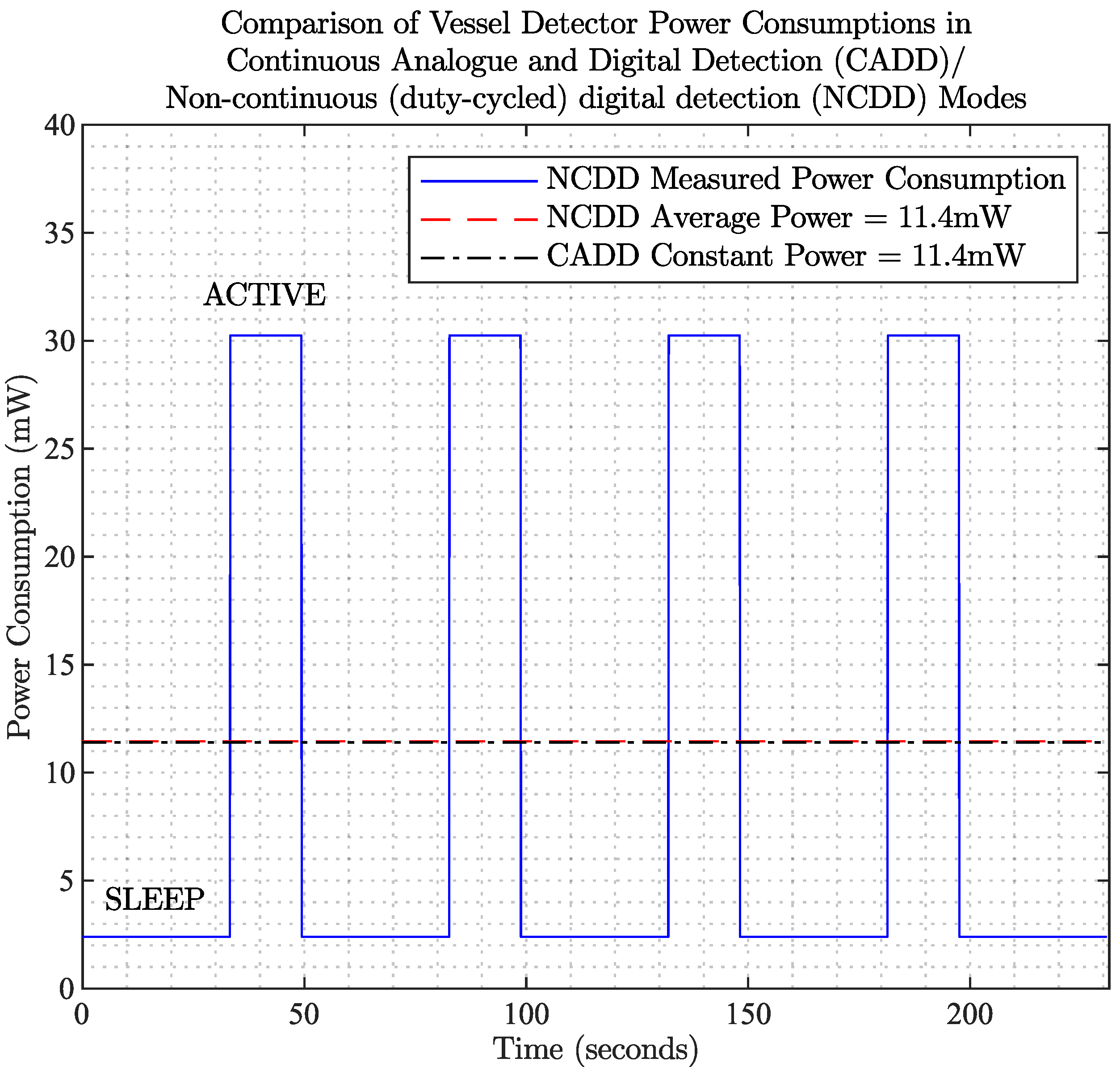
Unfortunately, COVID-19 has had an impact on this project’s timeline and ability to carry out all of the intended field trials. The vessel detector’s NCDD mode was planned to be deployed in open sea similar to that of the CADD mode. However, initial laboratory-based tests were been carried out to explore the NCDD power consumption and sensitivity when compared with the CADD mode. Figure 25 shows that both CADD and NCDD modes have been designed to have a matched average level of power consumption.
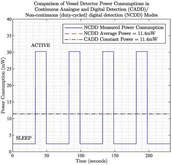
Figure 25.
Power consumption comparison between the vessel detector’s CADD and NCDD modes.
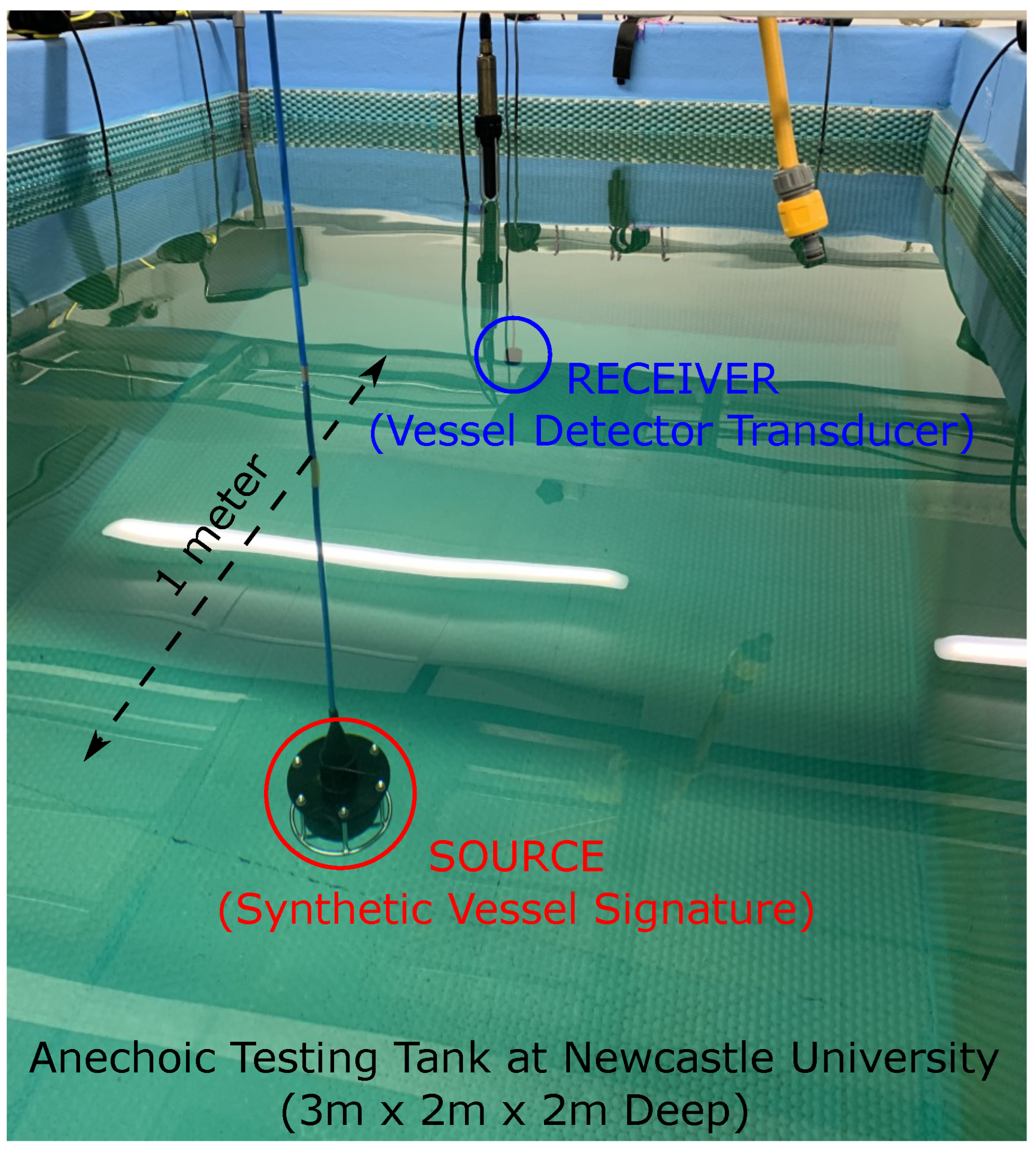
The reason for this is to explore whether a fully digital duty-cycled approach would perform better or worse than a continuous analogue/digital approach with the same power budget. Although open sea trials have not taken place to fully evaluate this question, Figure 26 shows a sensitivity experiment designed to give an indication.

Figure 26.
Experimental setup to evaluate the sensitivity difference between the vessel detector’s CADD and NCDD modes.
The experiment uses a synthetic vessel signal at the source to trigger the vessel detector at the receiver. The source signal used was a 32 sine wave with 20 sinusoidal amplitude modulation at 100% depth. The source signal remains constant in all aspects aside from the amplitude, which is reduced incrementally. Using this gradually attenuated signal, it is possible to measure the point at which the vessel detector fails to detect the synthetic vessel signal. This was carried out using both NCDD and CADD modes. As expected, the fully digital version showed a superior minimum detection level of −21.9 dB, with the CADD mode minimum detection level being −16.5 dB. This implies that the NCDD mode could achieve a greater detection radius in open sea for the same power budget. The question still remains what impact a duty-cycled approach will have on the accuracy of detection results, which forms part of the future work of this project.
4. Case Studies
4.1. Validation Field Trial—North Sea, December 2020
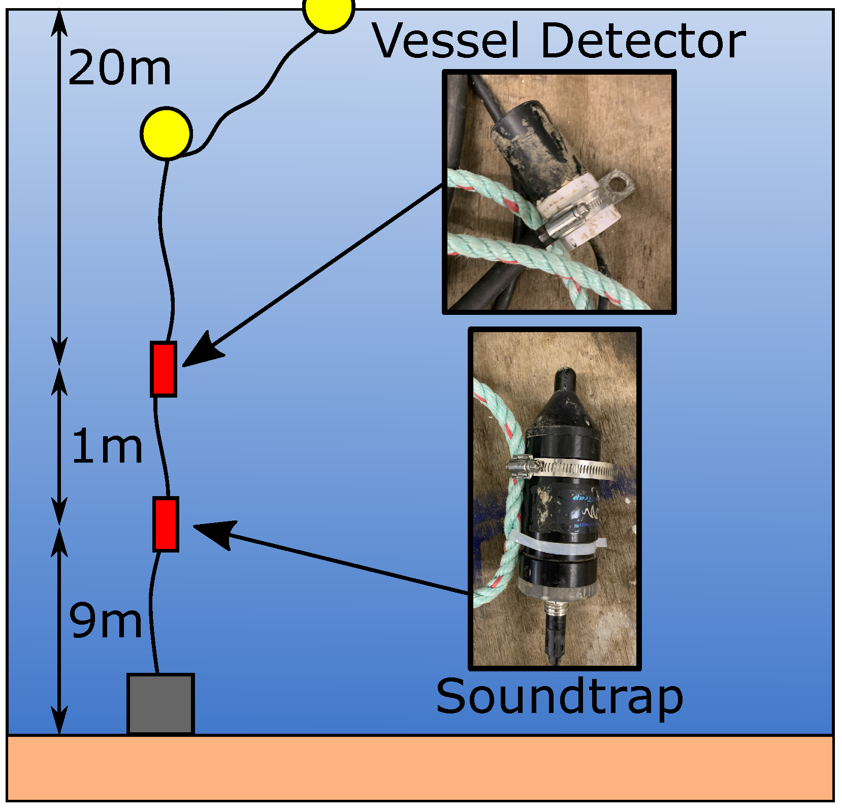
In this case study, a field trial was designed with the aim of validating the performance of the vessel detector as close to ground truth as possible. The trial utilised local AIS data alongside an underwater acoustic recorder situated on the same mooring as the vessel detector. The aim was to capture the raw acoustic signal as received by the vessel detector itself. The recorder also captured acoustic data transmissions and the corresponding acoustic acknowledgement messages from the gateway. This field trial was short in duration due to the limited recording capacity and battery life of the Soundtrap acoustic recorder. The setup of the field trial is illustrated in Figure 27.
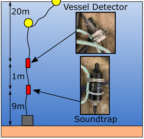
Figure 27.
Field trial illustration showing the mooring and equipment deployed.
The trial lasted 12 days in total. During this time there were 697 positive acoustic propeller cavitation events detected. A summary of the detection activity for the trial is shown in Figure 28.
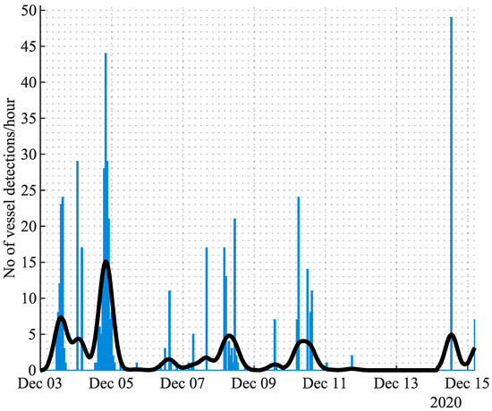
Figure 28.
This plot shows the number of vessel detections per hour for each day of the field trial.
To illustrate the ability of the system to reliably detect vessel activity when deployed at sea, one of the many detection events has been chosen to show data from all of the available monitoring equipment. The time period presented is on the 7 December 2020 between 16:23 and 16:48. The first data set considered is shown in Figure 29, which is local AIS data showing vessel activity in the area.
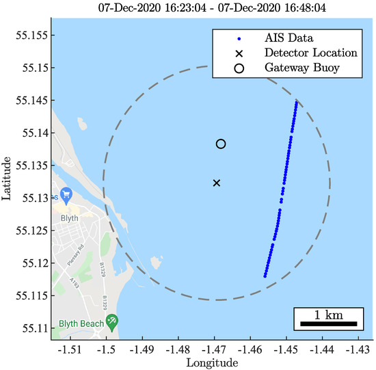
Figure 29.
Map of the vessel activity in the North Sea off the coast of Blyth for the given time period.
AIS data also provides information about the vessel itself based on the Maritime Mobile Service Identity (MMSI) number. Based on the MMSI number, a picture of the vessel detected is shown in Figure 30.
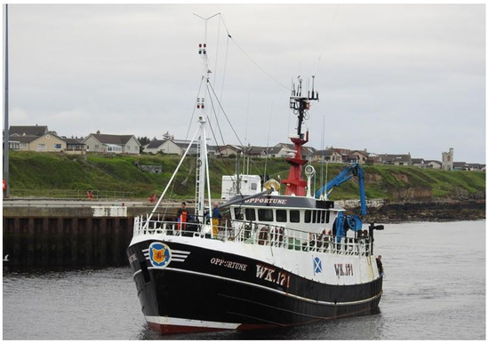
Figure 30.
Picture of the vessel detected during the time period of 16:23 and 16:48 on the 7 December 2020 based on the MMSI number provided by AIS data.
The next data set, shown in Figure 31, is a combination of the local AIS data and the vessel detection data received back at shore via the gateway buoy. The upper plot of Figure 31 shows when both AIS data and vessel detection data is present during the same time period, set at eight second intervals. The upper plot also shows the distance of the vessel based on AIS data. The lower plot in Figure 31 shows the detected peak frequency as a result of the DEMON algorithm. There is a general trend of 16 and 32 , which given their values, are likely to be the fundamental and harmonic frequencies. The change in peak magnitude intensity as shown by the colour change from light-dark-light is representative of a boat approaching and then leaving the detector’s area.
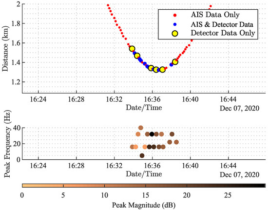
Figure 31.
Vessel detection and AIS data for the given time period. The upper plot compares the time stamp data of both the vessel detector and local AIS data. The lower plot shows peak magnitude/frequency data provided by the vessel detector as a result of the DEMON algorithm.
The final data source is the raw audio recorded by the Soundtrap device as shown in the field trial diagram in Figure 27. The device was set to record continuously for the duration of the trial at a sample rate of 96 kHz to capture propeller cavitation noise. Figure 32 shows a section of audio recorded during the field trial from the same time period as previous data sets. The plot shows both the time domain data as well as the frequency content of the recording. Looking at each plot, the acoustic data transmissions resulting from a positive detection are very apparent. These are the short duration, high-magnitude events towards the middle of each plot. The propeller cavitation emitted from the vessel is also visible in the spectrogram by looking for the faint sunburst-like pattern.

Figure 32.
Time/frequency plot of an audio recording taken during field trials on the 8 December 2020 between 05:22 and 05:37.
This pattern is further illustrated by expanding the spectrogram to look at a lower frequency band, as shown in Figure 33.
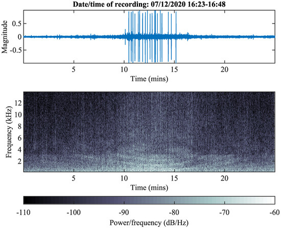
Figure 33.
Expanded view of Figure 32 to show the sunburst pattern of a vessel’s propeller cavitation emission.
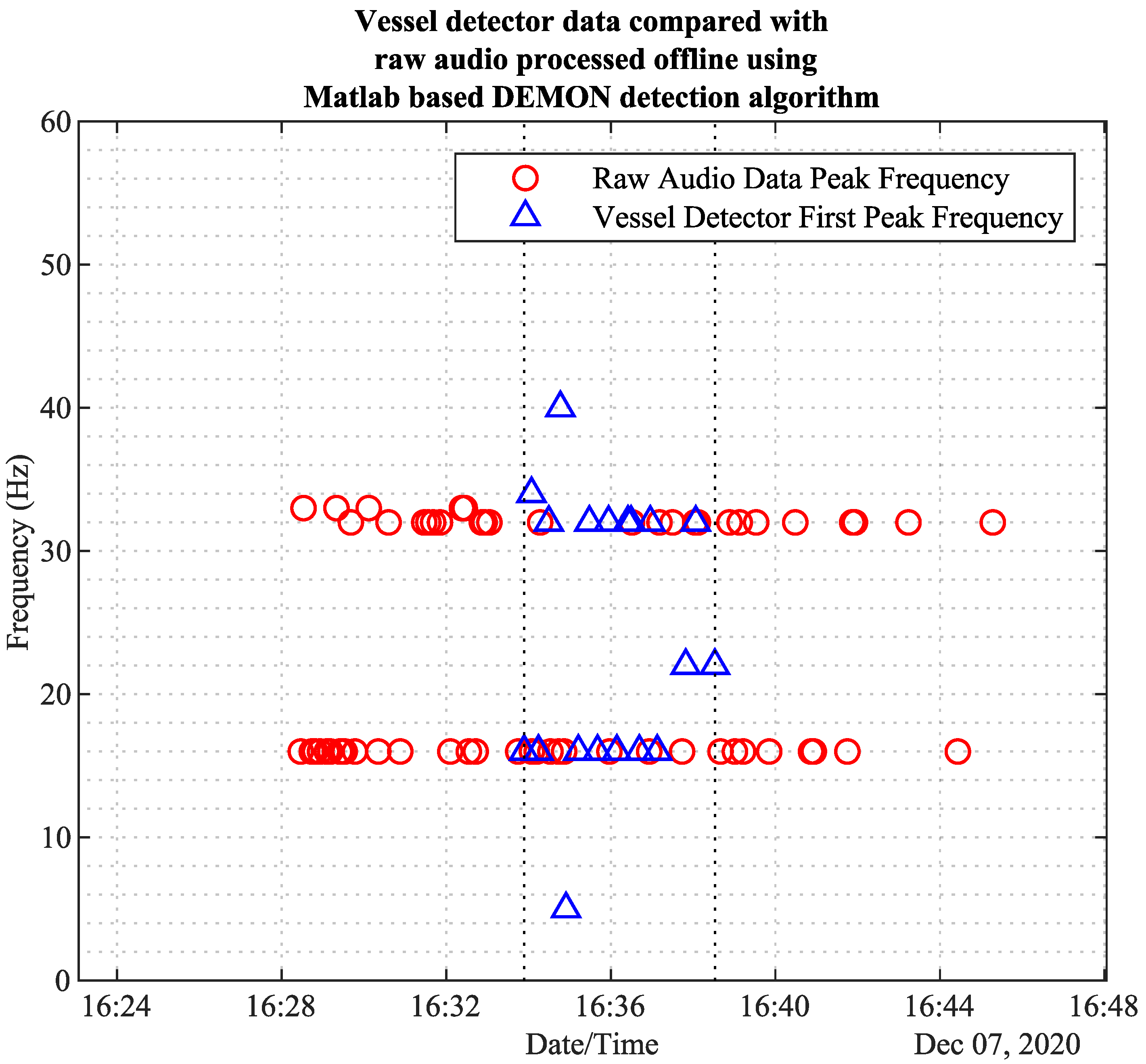
An additional method of validating the data produced by the vessel detector is to process the same period of raw audio through a Matlab-based version of the detection algorithm. The Matlab version of the detection algorithm benefits from a greater degree of FFT resolution as opposed to the fixed point FFT on the vessel detector. Matlab also processes data using floating point arithmetic; therefore, a high degree of accuracy is retained during calculation. Figure 34 shows a comparison of the Matlab-based algorithm and the original vessel detector data produced in the field. As shown, there is alignment for the detected peak frequencies of the vessel at 16 and 32 , with few outliers.
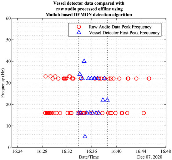
Figure 34.
Comparison of vessel detector data with raw audio processed by a Matlab-based version of the DEMON detection algorithm.
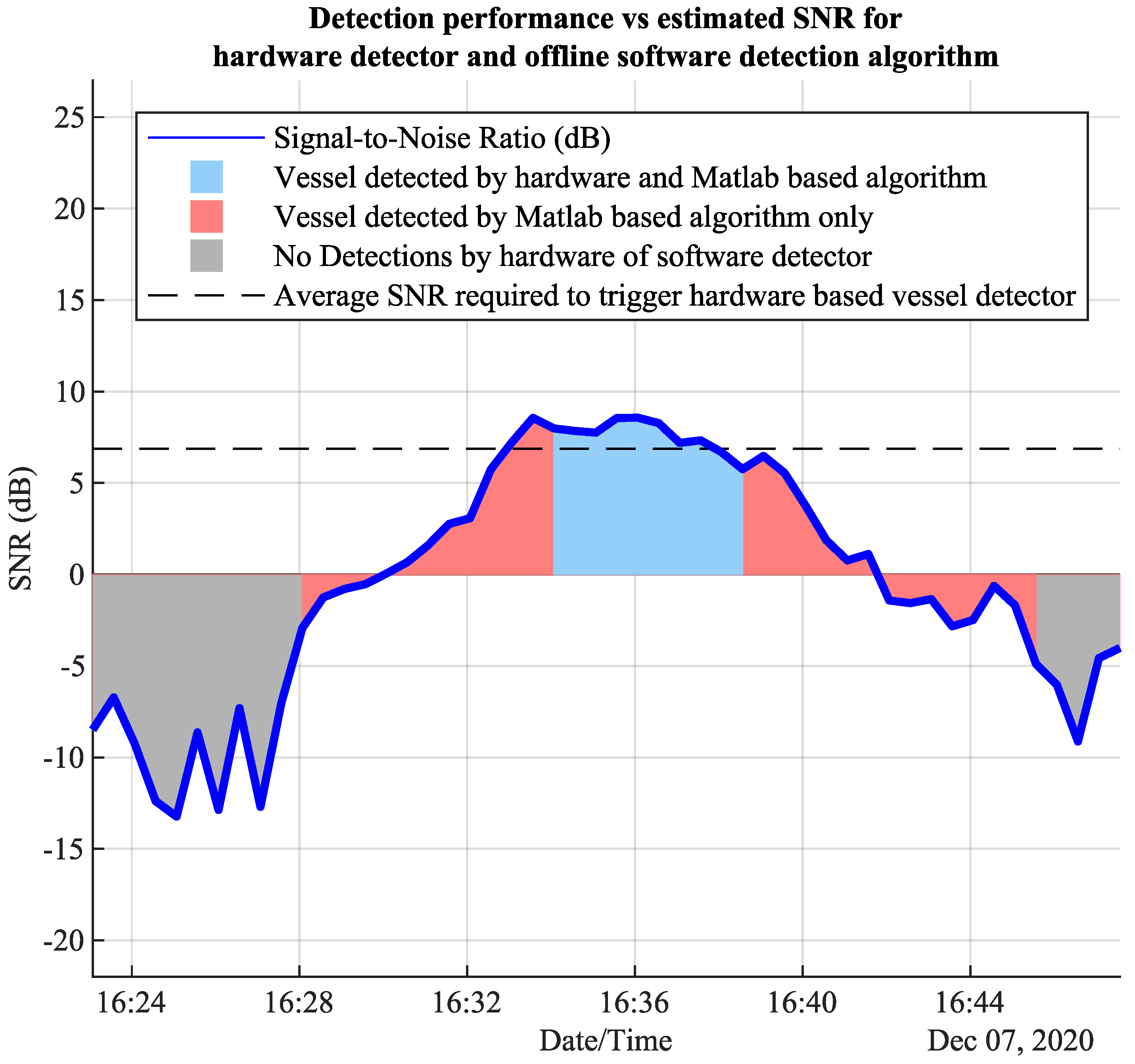
Using the Matlab-based detection algorithm and the fact that the raw audio processed is time aligned with the field detection data, it is possible to estimate the signal-to-noise ratio (SNR) required to trigger the vessel detector. In Figure 35, an estimation of the signal-to-noise ratio is calculated for 30 s intervals. The plot shows the timeframe when the hardware detector became active. The results show that an average SNR of 6.872 dB is required for the hardware-based detector to identify a vessel’s DEMON signature.
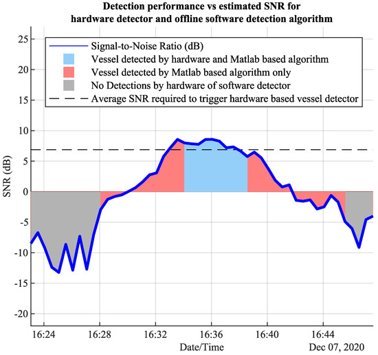
Figure 35.
Estimation of the signal-to-noise ratio (SNR) required for the vessel detector to operate.
Figure 35 also shows that a Matlab-based algorithm is able to detect the vessel much earlier than the vessel detector used in field trials. This is mainly due to the increased resolution and superior performance of the Matlab-based DEMON implementation. A low-energy implementation will inherently suffer from power/processing-based constraints, so there will always be a balance to strike when developing underwater wireless sensors.
As the Matlab algorithm results are based on a similar floating point-based arithmetic, the detection results in Figure 35 are representative of what the NCDD mode, presented in Section 3.7, could achieve in hardware.
In summary, this section shows data from three separate sources, which all provide strong evidence that a vessel was present during the monitoring timeframe. The vessel detector produced positive detections during the same time period in which both the AIS data and raw acoustic recording suggested that a vessel was present.
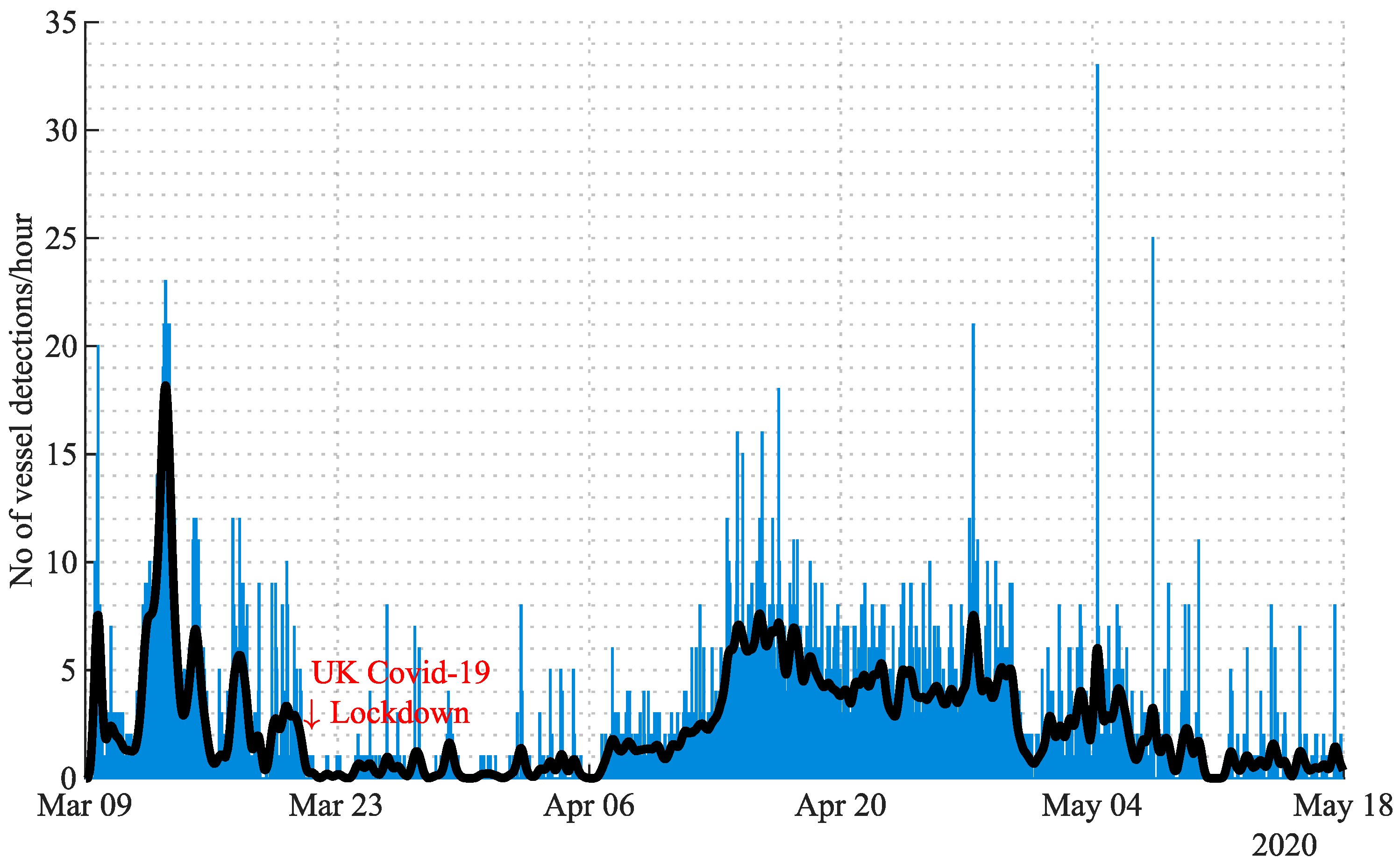
4.2. Impact of COVID-19 on North Sea Vessel Traffic
An interesting result which has emerged from the vessel detector’s open sea deployment is the impact of COVID-19 on vessel activity in the North Sea. In March 2020, the UK was placed in lockdown to mitigate the spread of the virus and during this time the detector was still active and communicating data. Looking at the results during this period, there appears to be an abrupt change in the data trend. Figure 36 shows that once the lockdown was put in place, there was very little vessel activity detected in contrast to the days and weeks prior. This reduction in activity was observed within the detection data for a duration of around two weeks. This detection data has been corroborated with vessel activity observed by the Northumberland Inshore Fisheries and Conservation Authority (NIFCA). The Environmental Inshore Fisheries and Conservation Officer at NIFCA explained the data that the vessel detector was producing around the lockdown period. The reason for the sharp reduction in activity was due to local fishery markets closing in response to the COVID-19 lockdown. The resurgence of activity after around a two-week period of lockdown was due to wholesalers beginning to buy shellfish again from fishermen 4 days per week [34]. This validation by local authorities gives great confidence in the vessel detector’s ability to reflect the number of vessels in the area and ultimately its ability to reliably detect vessels.

Figure 36.
Vessel detection data used to illustrate the impact of COVID-19 on local vessel activity in the Blyth area. The data shows the number of vessels detected per hour over a period of 5 months.
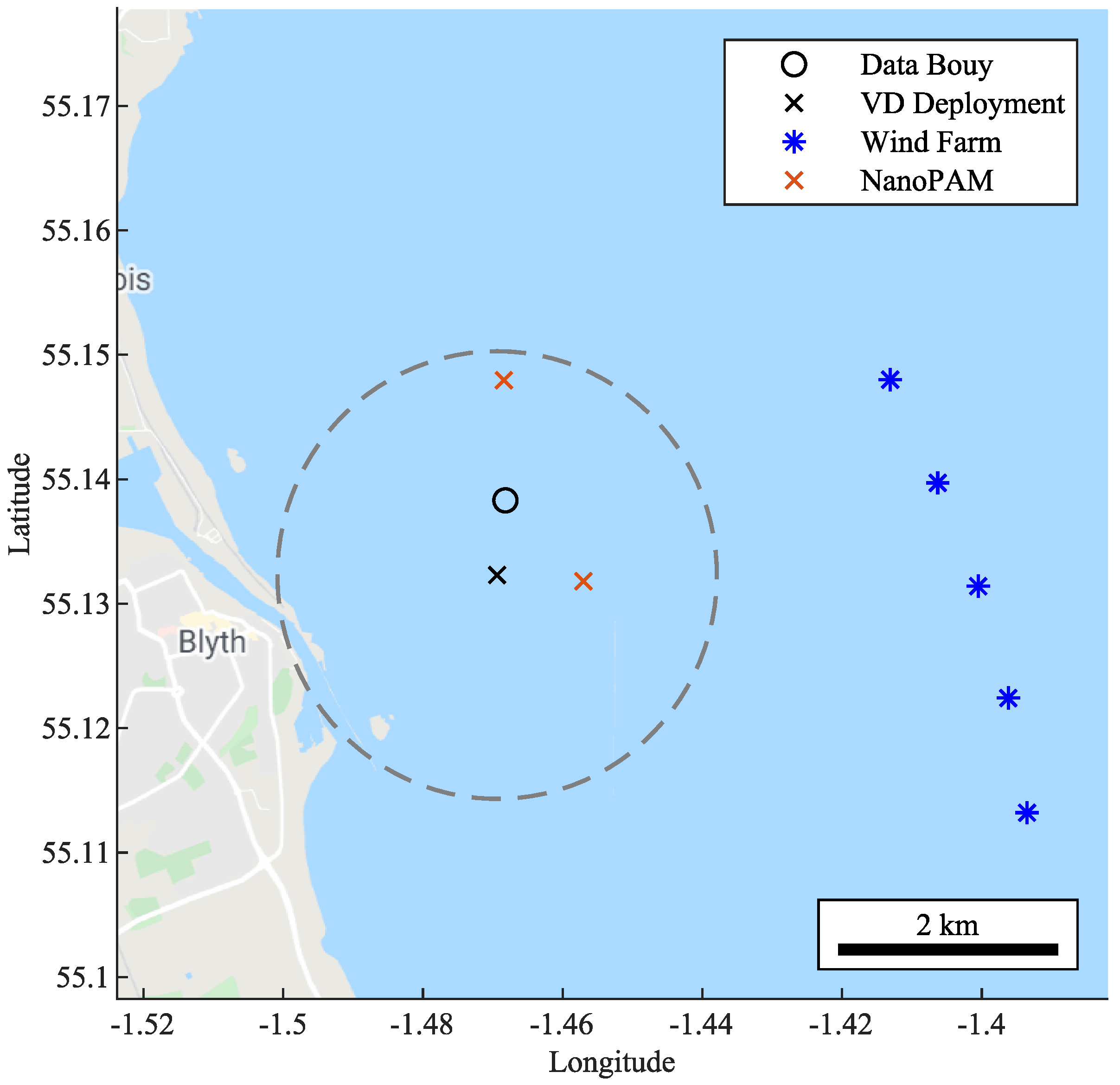
During March 2020, a sister project from SEALab, named NanoPAM, was operating in two locations near to the vessel detector deployment, as shown in Figure 37.
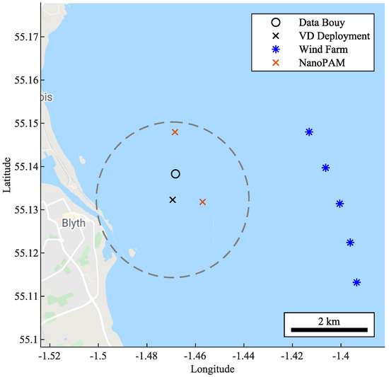
Figure 37.
Newcastle University SEA Lab field trial asset locations alongside the North Sea wind-farm for reference. A 2 km radius is provided around the vessel detector’s deployment location.
At these locations, two underwater audio recorders were active sampling at 576 . Using this data, the hourly average magnitude of noise in the band 1 to 20 can be calculated. Figure 38 shows the mean noise level of each recorder location, alongside the vessel detection data for the same period.
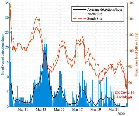
Figure 38.
Mean noise levels present during a period of vessel monitoring.
In Figure 38, there is a strong correlation between the north and south monitoring sites mean noise level. As these sites are approximately 2 apart, the data suggests that a single source is dominant in influencing the mean noise level. The most obvious assumption would be the weather conditions, as this would likely be consistent over a 2 area. Comparing the mean noise level with the vessel detection data, there is no consistent correlation between mean noise level and vessels detected. This suggests that noise level alone is not a reliable indicator for vessel activity and demonstrates the value of the DEMON-based detection device.
5. Conclusions
The aim of this project was to produce a low-energy passive acoustic vessel detector that can operate as part of a wireless underwater network.
Results demonstrated the vessel detector is able to reliably identify passing vessels based solely on the acoustic signature emitted during propeller cavitation. This has included detecting multiple vessels operating during the same time period.
Power consumption measurements alongside periodic battery monitoring data showed that the vessel detector is capable of deployments lasting 4–6 months using only four alkaline C cells. Additional battery packs and a modified enclosure could enable a longer deployment duration. The average power consumption was measured to be 11.4 mW during detection mode. This confirmed that all of the low-energy design constraints were successfully met.
Reliability of the vessel detector was demonstrated in a variety of ways, including noise rejection due to severe weather, detection reliability when compared with local AIS data, and enclosure integrity in harsh North Sea conditions. Moreover, the embedded software and custom circuitry proved robust over the duration of the field trial without any human intervention required.
Results have shown that during long-term field trials, 94% of results could be corroborated with local AIS data. Local AIS data was used as the best available ground truth, accepting that some smaller vessels are not required to transmit AIS data.
Different approaches to vessel detection were developed using a mixture of analogue/digital signal processing and a continuous/duty-cycled monitoring approach. Unfortunately, due to COVID restrictions, the duty cycled approach has yet to be tested at sea, but this forms part of future work. However, lab trials showed that with the same average power consumption as the CADD mode, the NCDD mode was able to detect vessel-like signals at a level 5.4 dB lower than the CADD mode. This is due to the improved performance of the digital envelope detection and filtering stages in the NCDD mode. This improved sensitivity has the potential to increase the detection radius and identify vessels further away from the node.
Future Work
As with much research during a global pandemic, there were disruptions to planned work. This means that some of the initial work planned will now form part of future work. Planned work includes testing the technology developed as part of a distributed network of underwater sensor nodes. This will give greater spatial data, which could offer the ability to not only detect vessels, but track them through the network. In addition, further testing of a duty cycled fully digital approach at sea may increase the detection sensitivity for the same energy budget as a continuous analogue/digital approach.
During field trials in the North Sea, there were many cetacean encounters recorded by our gateway buoy. These encounters have been verified by a sister project within the SEALab, which attempts to detect cetacean activity based on high-frequency click trains [35]. An interesting outcome of this data verification is that on occasion, there is a possibility that the vessel detector may have been fooled by slow cetacean click trains. High-energy short-duration clicks can produce an amplitude modulation on the analogue envelope detector output, which in turn appears on the DEMON spectrum. It is difficult to say for certain that these slow click trains are producing false positive results, as audio recordings were taken 1 km from the vessel detector’s location. Vessels were in the area during the encounter, but they were around 13 km south of the vessel detector.
One method of rejecting these potential false alarm sources would to examine the detected DEMON peak frequency over time. If the detection was a vessel, each of the detected peak frequencies would tend to show a consistent trend over time. This frequency trend can be extrapolated over a longer time duration for a vessel, as they tend to be continuously acoustically active for much longer than a cetacean. Dolphins and porpoises rapidly and erratically vary their inter-click interval (ICI) in response to their environment or the prey they are tracking, and this would appear on the DEMON spectrum. Such behaviour would be unusual for a vessel propeller (rapid/erratic throttle variations). A fully digital detector could also help to discriminate short clicks from envelope modulated broadband noise, as clicks demonstrate a high peak-to-average-power ratio.
Author Contributions
Conceptualisation, G.J.L. and J.N.; methodology, G.J.L. and J.N.; software, G.J.L.; validation, G.J.L.; formal analysis, G.J.L.; investigation, G.J.L.; resources, G.J.L., J.N., C.T., R.B. and B.S.; data curation, G.J.L. and B.S.; writing—original draft preparation, G.J.L.; writing—review and editing, G.J.L., J.N., C.T., R.B. and B.S.; visualisation, G.J.L.; supervision, J.N. and C.T.; project administration, G.J.L. and J.N.; funding acquisition, J.N. All authors have read and agreed to the published version of the manuscript.
Funding
This research was funded by the Engineering and Physical Sciences Research Council (EP/P017975/1).
Institutional Review Board Statement
Not applicable.
Informed Consent Statement
Not applicable.
Data Availability Statement
Not applicable.
Acknowledgments
The author would like to acknowledge the project sponsor, Engineering and Physical Sciences Research Council (EPSRC), for funding this project (EP/P017975/1). In addition, the author would like to thank the project collaborators, University of York, Herriet-Watt University, Technip FMC, Imenco UK Ltd, and Subsea 7. The author would like to give gratitude to Newcastle University and the staff at Blyth Marine station, Neil Armstrong and Barry Pearson, for their assistance during work undertaken at sea.
Conflicts of Interest
The authors declare no conflict of interest.
References
- Nunez, C. Find Out about the World’s Ocean Habitats and More. 2020. Available online: www.nationalgeographic.com (accessed on 11 January 2022).
- Dearden, L. Yacht ‘smuggling £60m of cocaine into UK’ seized off Welsh coast. The Independent, 28 August 2019. [Google Scholar]
- Environment Agency. Illegal fishing nets seized in Northumberland. Environment Agency, 3 June 2020. [Google Scholar]
- Gov. Royal navy shadows seven russian warships in the channel and north sea. Royal Navy, 26 March 2020. [Google Scholar]
- Specia, M. Migrants Crossing the English Channel to the U.K. Increased Sixfold in 2019. New York Times, 4 January 2020. [Google Scholar]
- Ryall, J. More migrants intercepted in Channel as numbers reach 1,000 since lockdown. ITV News, 20 May 2020. [Google Scholar]
- Johnson, J. More migrants have crossed the Channel illegally this year than the whole of 2019, as a record 166 arrive on nine boats. The Telegraph, 3 June 2020. [Google Scholar]
- BBC News. Channel migrants try to cross English Channel in fog. BBC News, 16 June 2020. [Google Scholar]
- Korosec, M. Severe windstorm will push into S England, English Channel. Severe Weather Europe, 1 November 2019. [Google Scholar]
- Bhattacharjee, S. Automatic Identification System (AIS): Integrating and Identifying Marine Communication Channels. Marine Insight, 31 December 2019. [Google Scholar]
- Gov. Automatic Identification System (AIS) for fishing vessels. Marine Management Organisation, 12 August 2014. [Google Scholar]
- Lowes, G.J. Low Energy, Passive Acoustic Sensing for Wireless Underwater Monitoring Networks. Ph.D. Thesis, School of Engineering, Newcastle University, Newcastle upon Tyne, UK, 2021. [Google Scholar]
- Abrahamsen, K. The ship as an underwater noise source. In Proceedings of the Meetings on Acoustics ECUA2012, ASA, Edinburgh, UK, 2–6 July 2012; Volume 17, p. 070058. [Google Scholar]
- Ross, D. Mechanics of Underwater Noise; Peninsula: Los Altos, CA, USA, 1987. [Google Scholar]
- Carlton, J. Marine Propellers and Propulsion, 2nd ed.; Butterworth-Heinemann: Oxford, UK, 2007. [Google Scholar]
- Lowes, G.J.; Neasham, J.A.; Burnett, R.; Tsimenidis, C.C. Low Energy, Passive Acoustic Sensing for Wireless Underwater Monitoring Networks. In Proceedings of the OCEANS 2019 MTS/IEEE SEATTLE, Seattle, WA, USA, 27–31 October 2019; pp. 1–9. [Google Scholar]
- Merchant, N.D.; Brookes, K.L.; Faulkner, R.C.; Bicknell, A.W.; Godley, B.J.; Witt, M.J. Underwater noise levels in UK waters. Sci. Rep. 2016, 6, 36942. [Google Scholar] [CrossRef] [PubMed]
- Averbuch, A.; Zheludev, V.; Neittaanmäki, P.; Wartiainen, P.; Huoman, K.; Janson, K. Acoustic detection and classification of river boats. Appl. Acoust. 2011, 72, 22–34. [Google Scholar] [CrossRef]
- Sorensen, E.; Ou, H.H.; Zurk, L.M.; Siderius, M. Passive acoustic sensing for detection of small vessels. In Proceedings of the OCEANS 2010 MTS/IEEE SEATTLE, Seattle, WA, USA, 20–23 September 2010; pp. 1–8. [Google Scholar]
- Chung, K.W.; Sutin, A.; Sedunov, A.; Bruno, M. DEMON acoustic ship signature measurements in an urban harbor. Adv. Acoust. Vib. 2011, 2011, 952798. [Google Scholar] [CrossRef] [Green Version]
- Clark, P.; Kirsteins, I.; Atlas, L. Multiband analysis for colored amplitude-modulated ship noise. In Proceedings of the 2010 IEEE International Conference on Acoustics, Speech and Signal Processing, Dallas, TX, USA, 14–19 March 2010; pp. 3970–3973. [Google Scholar]
- Pollara, A.; Sutin, A.; Salloum, H. Improvement of the Detection of Envelope Modulation on Noise (DEMON) and its application to small boats. In Proceedings of the OCEANS 2016 MTS/IEEE Monterey, Monterey, CA, USA, 19–23 September 2016; pp. 1–10. [Google Scholar]
- Pollara, A.; Sutin, A.; Salloum, H. Modulation of high frequency noise by engine tones of small boats. J. Acoust. Soc. Am. 2017, 142, EL30–EL34. [Google Scholar] [CrossRef] [PubMed] [Green Version]
- Sutin, A.; Salloum, H.; DeLorme, M.; Sedunov, N.; Sedunov, A.; Tsionskiy, M. Stevens passive acoustic system for surface and underwater threat detection. In Proceedings of the 2013 IEEE International Conference on Technologies for Homeland Security (HST), Waltham, MA, USA, 12–14 November 2013; pp. 195–200. [Google Scholar]
- USMART. Newcastle University USMART Project. 2021. Available online: www.research.ncl.ac.uk/usmart/ (accessed on 11 January 2022).
- Morozs, N.; Mitchell, P.; Zakharov, Y.V. TDA-MAC: TDMA without clock synchronization in underwater acoustic networks. IEEE Access 2017, 6, 1091–1108. [Google Scholar] [CrossRef]
- Morozs, N.; Mitchell, P.D.; Zakharov, Y. Routing strategies for dual-hop TDA-MAC: Trade-off between network throughput and reliability. In Proceedings of the Underwater Acoustics Conference & Exhibition, York, UK, 30 June–5 July 2019. [Google Scholar]
- Mourya, R.; Saafin, W.; Dragone, M.; Petillot, Y. Ocean monitoring framework based on compressive sensing using acoustic sensor networks. In Proceedings of the OCEANS 2018 MTS/IEEE Charleston, Charleston, SC, USA, 22–25 October 2018; pp. 1–10. [Google Scholar]
- Sherlock, B.; Neasham, J.A.; Tsimenidis, C.C. Spread-spectrum techniques for bio-friendly underwater acoustic communications. IEEE Access 2018, 6, 4506–4520. [Google Scholar] [CrossRef]
- Pollara, A.; Sutin, A.; Salloum, H. Passive acoustic methods of small boat detection, tracking and classification. In Proceedings of the 2017 IEEE International Symposium on Technologies for Homeland Security (HST), Waltham, MA, USA, 25–26 April 2017; pp. 1–6. [Google Scholar]
- Google. Google Maps. 2020. Available online: www.google.com/maps (accessed on 11 January 2022).
- Channel Coastal Observatory. 2020. Available online: www.coastalmonitoring.org (accessed on 11 January 2022).
- Ocean Instruments NZ SoundTrap 300—A Compact Self-Contained Underwater Sound Recorders for Ocean Acoustic Research. Available online: http://www.oceaninstruments.co.nz/soundtrap-300/ (accessed on 8 June 2020).
- Northumberland Inshore Fisheries and Conservation Authority (NIFCA). Available online: https://www.nifca.gov.uk/about/ (accessed on 8 June 2020).
- Berggren, P.; Neasham, J.A. Novel Low-Cost Methods for Marine Mammal and Environmental Monitoring, Project Reference: NE/R014884/1. 2020. Available online: www.ukri.org (accessed on 11 January 2022).


Publisher’s Note: MDPI stays neutral with regard to jurisdictional claims in published maps and institutional affiliations. |
© 2022 by the authors. Licensee MDPI, Basel, Switzerland. This article is an open access article distributed under the terms and conditions of the Creative Commons Attribution (CC BY) license (https://creativecommons.org/licenses/by/4.0/).