An AUV Target-Tracking Method Combining Imitation Learning and Deep Reinforcement Learning

Abstract

This study aims to solve the problem of sparse reward and local convergence when using a reinforcement learning algorithm as the controller of an AUV. Based on the generative adversarial imitation (GAIL) algorithm combined with a multi-agent, a multi-agent GAIL (MAG) algorithm is proposed. The GAIL enables the AUV to directly learn from expert demonstrations, overcoming the difficulty of slow initial training of the network. Parallel training of multi-agents reduces the high correlation between samples to avoid local convergence. In addition, a reward function is designed to help training. Finally, the results show that in the unity simulation platform test, the proposed algorithm has a strong optimal decision-making ability in the tracking process.

1. Introduction

The autonomous underwater vehicle (AUV) is an unmanned underwater device programmed with a controller to perform its tasks automatically [1]. As an important tool for humans to understand the ocean, AUVs have been widely used for a variety of underwater tasks [2], such as subsea mapping [3], image processing [4,5,6], pipeline maintenance [7], and field source search [8]. AUVs have also been involved in scientific investigations of the ocean and lakes [9].

Control technology is an important part of AUV design. Linear controllers such as the PID and linear quadratic regulator are widely used in the fields of science and engineering [10,11] but have problems such as slow response and oscillation, which lead to being unstable for variations and AUV parameters in the environment [12,13]. Christudas et al. [14] proposed a non-linear long short-term memory recurrent neural network control algorithm. Zamfirache et al. [15] proposed a control method that combines the deep Q-learning (DQL) algorithm and the meta-heuristic gravitational search algorithm (GSA). Precup et al. introduced a series of data-driven, model-free controllers [16,17].

Reinforcement learning (RL) has achieved rapid development, such as aircraft control, factory scheduling tasks, and industrial process control in the community of autonomous control [18,19]. Compared with traditional control strategies, RL does not require prior knowledge of environmental model parameters and has strong adaptability and autonomous control capability [20]. The emergence of neural networks has enabled deep learning to achieve tremendous development in the communities of hyperspectral image classification, agricultural science, and biomedicine [21,22,23]. It also solved the problem that traditional RL algorithms such as Q-learning have of not being able to control agents in a high-dimensional state space and action space by introducing neural networks [24]. In addition, neural networks provide an efficient method for designing non-linear controllers [25]. Schulma et al. [26] proposed the proximal policy optimization (PPO) algorithm using neural networks, which can perform control tasks in a high-dimensional continuous action space. Haarnoja et al. [27] proposed a soft actor-critic (SAC) algorithm to make the agent explore as much as possible while completing the task by introducing entropy.

A problem in RL is that the rewards are sparse in some complex environments [28], which makes it difficult to obtain the positive reward at the beginning of training. Research shows that imitation learning (IL) learns to control strategies from demonstration trajectory samples and can solve the sparse reward problem [29]. In IL, the agent can obtain the information needed in the motion control process from the demonstration trajectory samples. IL algorithms have been applied in many fields, including human–computer interaction and machine vision [30,31]. IL is mainly divided into two categories: one is called the behavioral cloning (BC) algorithm, which learns expectation strategies directly from expert demonstration [32]. However, the generalization ability is poor and only applicable to limited data samples. The other is the inverse reinforcement learning (IRL) algorithm. It is suitable for areas where the reward function is difficult to quantify accurately [33]. However, it takes a long time to rebuild the reward function. The generative adversarial imitation learning (GAIL) algorithm can learn strategies directly from expert trajectories without restoring reward function by introducing generative adversarial networks (GAN) [34]. It greatly reduces the complexity of calculation and improves the shortcomings of long training times of the IRL algorithm.

Another problem in RL is that the data sample information generated is highly correlated, leading to local convergence. One solution to this problem is to perform random sampling in the experience replay buffer, but this solution is only suitable for off-policy RL [35]. Another solution is multi-agent RL. With the increase in the number of agents, the computational complexity of multi-agent RL also increases. Gupta et al. [36] proposed a parameter sharing trust-region policy optimization algorithm that combines parameter sharing and trust-region policy optimization (TRPO) to solve the problem of computational complexity. Multi-agent RL makes samples come from different AUVs to avoid the correlation of the samples [37].

The main contributions of this research are as follows: we propose a multi-agent GAIL (MAG) algorithm to control AUVs tracking the target. GAIL is used to help training, enabling AUVs to directly learn from expert demonstrations, solving the sparse reward problem. The high correlation of training samples through multi-agent RL will be reduced. Finally, the experiments show that the tracking effect of the proposed algorithm is better than PPO, SAC, and GAIL in three different environment models.

2. Problem Formulation

2.1. Coordinate Systems of AUVs

The coordinate system is shown in Figure 1. The study of the dynamics of AUV can be divided into two parts, which are kinematics and kinetics. Kinematics is used to describe the movement process of AUV, and dynamics represents the force received during the movement of AUV. This paper assumes that the target is moving in a two-dimensional plane on the seabed, so it is considered that the AUV only tracks the target in the plane. When describing the motion of the AUV, there are usually two sets of coordinate systems: the inertial coordinate system $\mathrm{O}-\mathrm{XYZ}$ and the motion coordinate system $o_a-uvw$. $(\xi ,\vartheta ,\zeta )$ represents the roll angle, pitch angle, and yaw angle of the AUV. $\left(u,v,w\right)$ are the turbulence speed, sway speed, and heave speed; $\left(p,q,r\right)$ are the roll angular velocity, pitch angular velocity and yaw angular velocity; and the point $\left(x_a,y_a,z_a\right)$ represents the position of the AUV in the inertial coordinate system.

The kinematic equation of AUV is as follows:

$$\stackrel{•}{\eta }=J(\zeta )\varphi ,$$

(1)

$$M\stackrel{•}{\varphi }+C(\varphi )\varphi +D(\varphi )\varphi =G(\varphi )\tau ,$$

(2)

$$J(\zeta )=\left(\begin{array}{ccc}\cos \zeta & -\sin \zeta & 0\\ \sin \zeta & \cos \zeta & 0\\ 0& 0& 1\end{array}\right)$$

(3)

where $\eta ={[x_a,y_a,z_a]}^T$ and $\varphi ={[u,v,w]}^T$, $M$ is the mass matrix, $C(\varphi )$ is the Coriolis–centripetal matrices, respectively, $D(\varphi )$ is the damping matrix, $G(\varphi )$ is the input matrix, $J(\varphi )$ is the transformation matrix, $\tau$ is the joint torques. The coefficients in $M$, $C(\varphi )$, $G(\varphi )$, $D(\varphi )$ are given [38]:

$$M=\left(\begin{array}{ccc}{m}_1& 0& 0\\ 0& m_2& m_3\\ 0& m_4& m_5\end{array}\right),$$

(4)

$$G(\varphi )=\left(\begin{array}{cc}1& 0\\ 0& g_1(\mu )\\ 0& g_2(\mu )\end{array}\right),$$

(5)

$$C(\varphi )=\left(\begin{array}{ccc}0& 0& c_1(v,r)\\ 0& 0& c_2(u)\\ -c_1(v,r)& -c_2(u)& 0\end{array}\right),$$

(6)

where $m_1~m_5$, $c_1$, $c_2$, $d_1~d_5$, $g_1$ and $g_2$ are unknown functions of hydrodynamic coefficient.

2.2. Problem Description

As shown in Figure 2, the trajectory of the target covers as much of the entire pool as possible, and the random noise is considered. Therefore, in the experiment, the trajectory curve of the target is set to circle the pool for periodic motion. In other words, the target is moving along the seafloor plane $\left\{w{p}_1\to w{p}_2\to w{p}_3\to w{p}_4\to w{p}_1\dots \right\}$; the point $\left(x_g,y_g\right)$ represents the position of the target in the inertial coordinate system.

The AUV is equipped with a light sensor. The light sensor aims to transmit the position of the target and the position of the AUV to the action–decision system, and then the strategy network outputs the action command according to the state of the AUV, and finally through the propeller power unit and the bias aerodynamic moment controls the AUV. The AUV may collide with the target during the tracking process, thereby changing the motion state of the target. The target is considered to be tracked by the AUV if the distance is less than a certain value, that is $\{x_a,x_g,y_a,y_g\in {\mathrm{R}}^2:{\left[{(x_a-x_g)}^2+{(y_a-y_g)}^2\right]}^{\frac{1}{2}}\le \epsilon \}$. The AUV tracking control can be described as the design algorithm to make the distance between the AUV and the target less than a certain value.

2.3. State Space and Action Space of AUV

The AUV obtains the observation vector from the state space as the input value of the neural network and provides the appropriate action for the AUV through the action–decision system to accurately track the target. Therefore, the selection principle of the observation vector is the state information needed to complete the task. In order to reduce the dimensionality of the state space as much as possible, the data information must be independent. As mentioned in the previous section, the state space is the position information of the target and the AUV. In the actual process, we normalize the value of the observation vector. This normalization is based on the mean and variance of the observation vector, thus speeding up the convergence of the neural network; the speed and direction of the AUV during the movement will determine the success or failure of the tracking task, so it is set as the action vector and also as the output of the neural network. It can be expressed as follows:

$$v_p=(u,\overrightarrow{P}),$$

(7)

where $u_a$ represents the velocity of AUV, and $\overrightarrow{P}$ represents the direction vector of the AUV towards the target.

3. MAG Path-Planning Algorithm

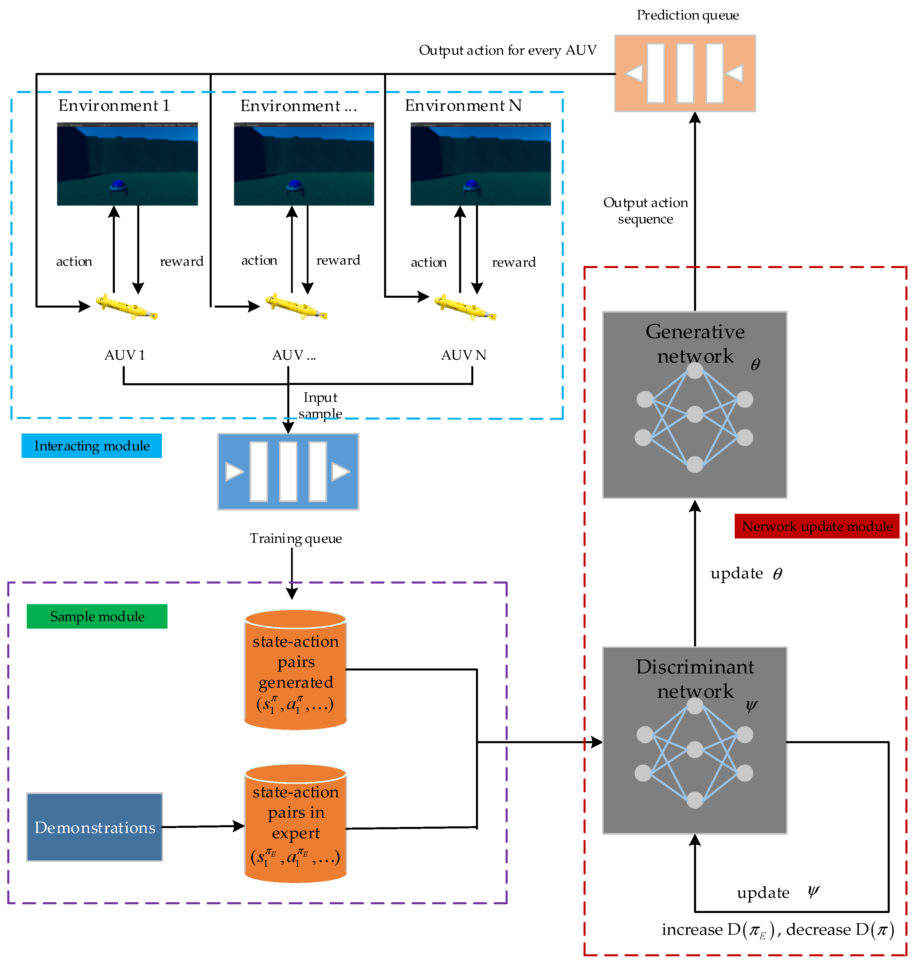
As shown in Figure 3, MAG consists of three modules. The first is the interaction module. The main function of this module is to interact with the environment to generate samples and output them to the training queue. The second is the sample module, which contains generated samples input from the training queue and expert samples input from the demonstration. The third is the network update module, which updates the discriminant network $D_{\psi }$ and the generative network $G_{\theta }$. After the update, it outputs the action sequence to the AUV waiting to execute the action. After the training is completed, the generator network $G_{\theta }$ is the controller of the AUV.

3.1. Markov Decision Process

A Markov process consists of quintuples $(S,A,T,R,\gamma )$. $S$ is the state space, which contains all the situations of the agent interacting with the environment; $A$ is the action space, which is the action performed by the agent from state $s$ to state $s^{\prime }$; T is the state transition model; $T(s^{\prime }|s,a)$ is the probability that the agent performs action $a$ in state $s$ and reaches state $s^{\prime }$; $R$ is the reward function, which provides rewards when the agent interacts with the environment; and $\gamma$ is the discount factor, which determines the current value of the rewards that the agent will obtain in the future.

3.2. Discriminant Network

GAIL defines IL as the problem of matching demonstrations of expert policies ${\pi }_E$ by introducing a GAN framework. Demonstration is a series of state–action pairs $\left\{s_1,a_1,s_2,a_2,\dots \right\}$ produced by the agent interacting with the environment. According to the implementation process of generative adversarial networks, first of all, it is necessary to build a generative network and a discriminant network. The discriminant network $D_{\psi }$ parameterized by $\psi$ is used to learn to distinguish whether trajectories are formed by experts or non-experts, whereas the generative network $G_{\theta }$ parameterized by $\theta$ continuously imitates the expert policy until the discriminant network $D_{\psi }$ cannot distinguish the source of the trajectory. The objective of GAIL is to optimize the function [39]:

$$\underset{\theta }{\min } \underset{\psi }{\max } E_{{\pi }_E}\log D_{\psi }\left(s,a\right)+E_{{\pi }_{\theta }}\log \left(1-D_{\psi }\left(s,a\right)\right)$$

(8)

The discriminant network $D_{\psi }$ is to learn to output a high score when encountering a state–action pair from ${\pi }_E$ and a low score when encountering a state–action pair from samples. When $\pi$ is similar to gradually ${\pi }_E$, the scores of the outputs are gradually approached.

3.3. Generative Network

The generative network $G_{\theta }$ is a strategy network whose input is a state, and the output is an action, so it can generate state–action pairs. It uses PPO to perform generative network updates; since the step size is limited by the size of the control range, it can be updated smoothly when the variance of the reward value is large [26], and the limit of this range is controlled by the Kullback–Leibler (KL) divergence. The generative network can be stably updated by restricting the KL divergence of the new and old generative networks within a certain constraint range, as shown in Equation (9):

$$D_{KL}^{\max }\left({\pi }_{old},\pi \right)\le \delta$$

(9)

where $D_{KL}^{\max }\left({\pi }_{old},\pi \right)$ is the KL divergence of the old and new strategies, and $\delta$ is the constraint parameter of the KL divergence.

The original GAIL uses the output of the discriminant network as an alternative reward function. In order to speed up the training speed and compare with the RL algorithm, an incomplete reward function was added which only contains a few situations. The objective that the policy network needs to optimize is shown in Equation (10):

$$\underset{\theta }{\mathrm{maximize}} E_{s,a~{\pi }_{\theta }}\left[\log (D_{\psi }(s,a))+\frac{{\pi }_{{}_{\theta }}(a|s)}{{\pi }_{{}_{{\theta }_{old}}}(a|s)}{A}_{\theta }(s,a)\right]-D_{KL}^{\max }\left({\pi }_{{}_{{\theta }_{old}}},{\pi }_{\theta }\right)$$

(10)

where $E_p$ is accumulated reward value, $A_{\theta }(s,a)$ is the advantage function for the ${\pi }_{\theta }$.

3.4. Multi-Agent Training

AUVs in multiple identical environments share the same set of network parameters, and their decision-making does not affect one another. Two queues are included in the training: the prediction queue and training queue.

The prediction queue inputs all current AUV prediction requests into the generative network. After the prediction is completed, it transmits the requested action to each corresponding AUV that is waiting to execute the action.

The training queue submits the samples of the interaction between the AUV and the environment to the generative network and the discriminant network for parameters update. By collecting samples in multiple identical environments, the correlation between samples is reduced so as to avoid local convergence in the AUV training process.

3.5. Algorithm Process

According to the aforementioned methods, the algorithm process can be described as shown in Algorithm 1.

Algorithm 1. The path-plan training process.

Input: expert demonstrations $\left\{{\tau }_1^E,{\tau }_2^E,\dots ,{\tau }_N^E\right\}$. Create multiple identical underwater environments and create an AUV with light sensor and target in each environment in the unity software. Initialize training queue and prediction queue. Randomly initialize the discriminant network $D(s,a|\psi )$ and the generative network $G(s|\theta )$ while each AUV shares KL divergence and parameters of $D(s,a|\psi )$ and $G(s|\theta )$. for episode = 1 to M:  for step = 1 to N:   AUVs input state $s$ to training queue waiting for the output of action;   Generative network $G(s|\theta )$ output action sequences for prediction queue and obtains the generative trajectory $\left\{{\tau }_1,{\tau }_2,\dots ,{\tau }_N\right\}$;   Batch generative trajectory $\left\{{\tau }_1,{\tau }_2,\dots ,{\tau }_N\right\}$;   Step = step + 1;   If (hit the target or obstacle):    Calculate cumulative rewards;    break;  end for;  The discriminant network $D(s,a|\psi )$ scores generative trajectory $\left\{{\tau }_1,{\tau }_2,\dots ,{\tau }_N\right\}$;  Update the generative network $G(s|\theta )$ parameters ${\theta }_i$ to ${\theta }_{i+1}$ by maximizing Equation (10);  Update the discriminant network $D(s,a|\psi )$ parameters ${\psi }_i$ to ${\psi }_{i+1}$ by maximizing Equation (8);  Episode = episode + 1; end for; Output: the trained generative network to the AUV as a controller.

4. Experiments

4.1. Environmental Model and Training Parameters

In this section, simulation experiments were used to verify the performance of AUV subsea dynamic target tracking. Unity software was used to visually simulate the underwater environment. The motion model of the target and ocean current disturbance were written based on script languages with C# and Python. The generative network and discriminant network were constructed by the machine language library (Pytorch), and the model was trained by GPU. The experiment used AMD Ryzen 7 2700 Eight-Core 3.2 GHz processor (AMD Inc., Santa Clara, CA, USA) and 8 GB RAM graphics card. The overall experimental environment was an underwater environment of 25.0 × 25.0 × 1.0 m. This paper demonstrates the tracking effect of the controller in three scenes: Scene 1 is without obstacle and disturbance; Scene 2 is without obstacle and with disturbance; and Scene 3 is with four obstacles and without disturbance. The experiment set the center of the underwater environment as the origin $\left(0,0\right)$. The positions of the obstacles were $\left(-10,-10\right)$, $\left(-10,10\right)$, $\left(10,-10\right)$ and $\left(10,10\right)$. During training, the agent observed the environment using the light sensor; the angle range was $\{-60,60\}$, and the farthest distance measurement was 1.5 m.

In an iterative round process, set initial reward $R_0=0$, while the AUV obtains a −0.001 reward per step to speed up training. The round ends when the following three situations occur:

• The AUV collides with the target and gets a 0.1 reward.
• The AUV collides with an obstacle and gets a −0.1 reward.
• The AUV has completed 1000 steps. It can be expressed as follows:

$$R_j=\{\begin{array}{l}1.0+R_{j-1} \mathrm{if} \mathrm{track} \mathrm{the} \mathrm{target}\\ -0.1+R_{j-1} \mathrm{if} \mathrm{collide} \mathrm{the} \mathrm{obstacle}\\ R_{j-1}-0.001 \mathrm{other} \mathrm{else}\end{array},$$

(11)

where $j=1,2,\dots ,1000$, the episode ends on collision or tracking, or when the number of iterations $j$ reaches 1000, the accumulated reward at this time is recorded. Then, the parameters are reinitialized and the next round starts.

The parameters of the algorithm were set according to previous work [40,41,42], and the experimental conditions such as random noise and obstacles were also considered. The parameters of the PPO were set as: the sizes of batch, buffer, and memory were 128, 2048, and 256, respectively; the learning rate was 0.0001; the discount factor was 0.9; the epsilon was 0.2; the hidden layers were 2; and the hidden units were 256. The SAC parameters were as follows: the sizes of batch, buffer, and memory were 128, 2048, and 256, respectively; the discount factor was 0.9; the learning rate was 0.0003; the hidden layers were 2; and the hidden units were 256. The GAIL parameters were as follows: the sizes of batch, buffer, and memory were 64, 2048, and 256, respectively; the discount factor was 0.9; the epsilon was 0.2; the hidden layers were 2; the hidden units were 128; and the learning rate was 0.0001. The MAG parameters were as follows: the sizes of batch, buffer, and memory were 64, 2048, and 256, respectively; the discount factor was 0.9; the epsilon was 0.2; the hidden layers were 2; the hidden units were 128; the learning rate was 0.0003; and the sequence length was 64.

Perform 2000 Monte Carlo simulations for the four methods respectively, and the distance of the AUV and target is defined as follows:

$$d_i={\left[{(x_{a_i}-x_{g_i})}^2+{(y_{a_i}-y_{g_i})}^2\right]}^{\frac{1}{2}},$$

(12)

$$\stackrel{-}{d}=\frac{1}{N}{\displaystyle \sum _{i=1}^N{d}_i},$$

(13)

$$Va{r}_d=\frac{{{\displaystyle \sum _{i=1}^N\left(d_i-\stackrel{-}{d}\right)}}^2}{N-1},$$

(14)

where $i=1,2,\dots ,N$, and $N=2000$ is the number of Monte Carlo simulations. $(x_{a_i},y_{a_i})$ and $(x_{g_i},y_{g_i})$ are the corresponding coordinates of the AUV and the target, respectively.

4.2. Evaluation Standard

In general, the performance of the AUV controller is based on the cumulative reward, training time, the motion path of the AUV and the target, and the number of collision violations (CV) [43,44,45,46,47]. The reward is obtained by the AUV from the environment during training. The higher the cumulative reward, the more tasks the AUV will complete. The training time represents the computational complexity of a controller. The motion path represents the tracking accuracy of the controller during the entire movement process, and the CV represents the AUV’s ability to avoid obstacles.

4.3. Results

In order to verify the effectiveness of the algorithm proposed in this paper, the novel control algorithms of PPO, SAC, and GAIL were selected for comparison. PPO is a classic online RL algorithm that can be used to solve the sequential decision-making problem of unmanned aerial vehicles and non-linear attitude control problems [40,48]. SAC is a representative algorithm of offline RL that can realize low-level control of quadrotors and map-free navigation and obstacle avoidance of hybrid unmanned underwater vehicles [49,50]. GAIL is a representative IL algorithm that predicts airport-airside motion of aircraft-taxi trajectories and enables mobile robots to learn to navigate in dynamic pedestrian environments in a socially desirable manner [51,52].

From

Table 1. Data analysis of total reward using four methods in Scenes 1 and 2; ${\mathit{R}}_{max}$, ${\mathit{R}}_{min}$, ${\mathit{R}}_{ave}$ and ${\mathit{R}}_{var}$ shows the maximum, minimum, average value, and variance of the reward during training.

	Scene 1				Scene 2
	${\mathit{R}}_{\mathit{m}\mathit{a}\mathit{x}}$	${\mathit{R}}_{\mathit{m}\mathit{i}\mathit{n}}$	${\mathit{R}}_{\mathit{a}\mathit{v}\mathit{e}}$	${\mathit{R}}_{\mathit{v}\mathit{a}\mathit{r}}$	${\mathit{R}}_{\mathit{m}\mathit{a}\mathit{x}}$	${\mathit{R}}_{\mathit{m}\mathit{i}\mathit{n}}$	${\mathit{R}}_{\mathit{a}\mathit{v}\mathit{e}}$	${\mathit{R}}_{\mathit{v}\mathit{a}\mathit{r}}$
PPO [48]	1.0264	0.6773	0.9257	0.0035	1.0100	−0.4310	0.8753	0.0285
SAC [50]	0.9955	0.4053	0.9518	0.0121	0.9950	0.0591	0.9454	0.0220
GAIL [51]	0.9968	0.5482	0.9651	0.0057	0.9990	0.2442	0.9580	0.0147
MAG (Ours)	1.0031	0.8119	0.9861	0.0012	1.0032	0.1952	0.9548	0.0165

, it can be seen that the average cumulative reward of MAG is higher than PPO, SAC, and GAIL. The target-tracking task was completed more times, indicating that the MAG has the better performance in Scene 1. It can also be seen that the variance of MAG is lower than that of PPO and SAC, indicating that MAG can make the training process more stable. Compared to GAIL, the mean and variance are slightly lower than MAG.

By analyzing

Table 2. Training time and collision violations (CV) using PPO, SAC, GAIL, and MAG in the process of AUV target-tracking in Scenes 1, 2, and 3.

Index	Scene	Algorithm
		PPO [48]	SAC [50]	GAIL [51]	MAG (Ours)
Time(s)	Scene 1	1359.3	2857.7	1600.4	2558.1
	Scene 2	1716.1	3234.2	1583.1	2667.3
	Scene 3	1554.4	2843.8	1623.7	2644.2
CV	Scene 3	4	4	2	1

, it can be observed that MAG needs to spend the most time training. It improves obstacle avoidance while increasing the computational complexity.

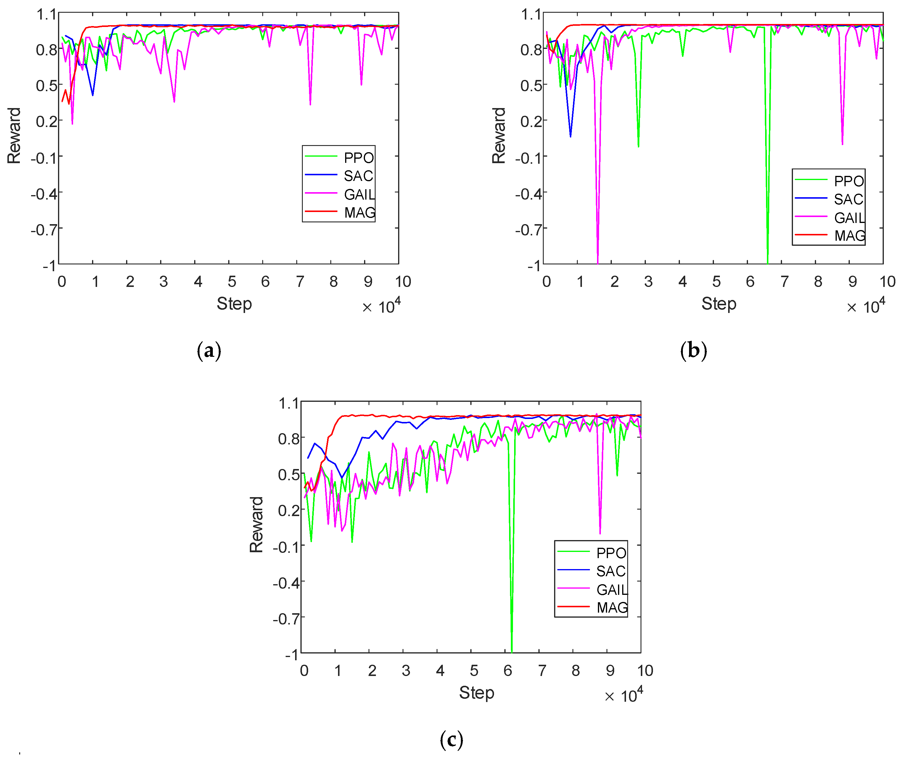
As shown in Figure 4, although the four methods can finally converge to around 1.0 after training 100,000 steps, the curve fluctuation range indicates that MAG has better stability during the training process and the network update is more stable. In Scene 2, the reward curve of the other three methods oscillates more obviously, indicating that MAG has better anti-disturbance after being affected by the ocean current. It can be seen from Figure 4c that the reward of the four methods reduced after Scenes 1 and 2 following the addition of obstacles, but the MAG controller still converges the fastest and updates the smoothest.

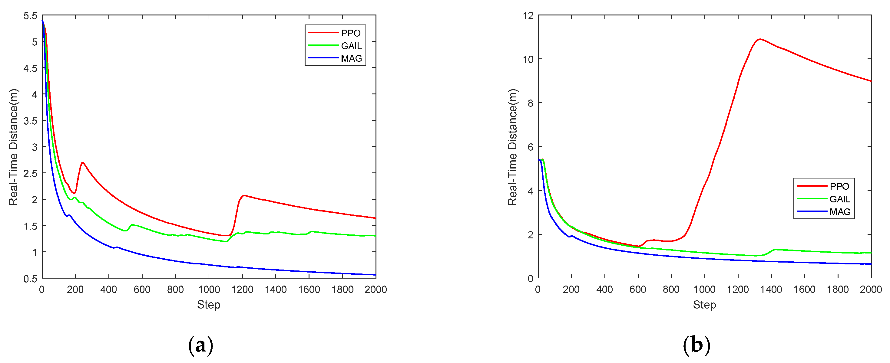
Figure 5 shows the change process of the distance between the AUV and the target. When there is no noise, the three algorithms can gradually decrease this distance. The MAG can bring the AUV closer to the target than PPO and GAIL. After adding noise interference, the distance was always kept at a high value when using PPO. However, the AUV controlled by MAG and GAIL could still track the target well. This shows that the anti-interference ability of MAG and GAIL is better than that of PPO.

In

Table 3. Comparison of tracking performance after AUV training 100,000 times using PPO, GAIL, and MAG in Scenes 1 and 2.

	Scene 1			Scene 2
	PPO [48]	GAIL [51]	MAG (Ours)	PPO [48]	GAIL [51]	MAG (Ours)
$\stackrel{-}{d}$	1.9280	1.5436	0.9630	5.7500	1.5337	1.1443
$Va{r}_d$	0.3661	0.3447	0.4073	13.7991	0.6411	0.5592
$\stackrel{-}{x_a}$	−7.1558	2.6253	8.5715	−2.0401	0.3701	−9.0751
$\stackrel{-}{y_a}$	5.9853	3.6069	8.5584	−0.1301	10.1977	−1.3942
$\stackrel{-}{x_g}$	−8.3558	2.9713	9.9069	1.1671	0.5142	−9.1093
$\stackrel{-}{y_g}$	6.0639	3.5525	9.4420	4.1045	9.8918	−2.4282

, $(\stackrel{-}{x_a},\stackrel{-}{y_a})$ is the average value of the coordinates of the AUV, $(\stackrel{-}{x_g},\stackrel{-}{y_g})$ is the average value of the coordinates of the target. The three algorithms are used in different underwater scenes to control the AUV to form the tracking trajectory. Compared with PPO and GAIL, the AUV controller by MAG is closer to the target and has better stability.

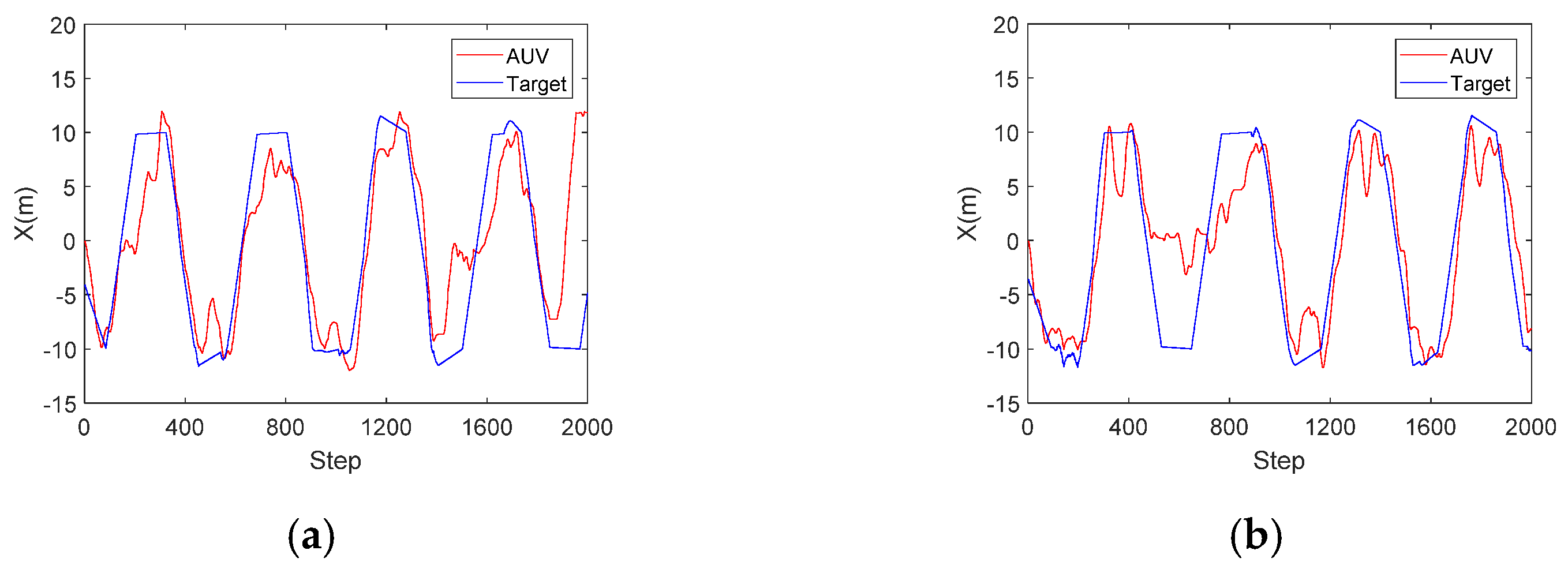
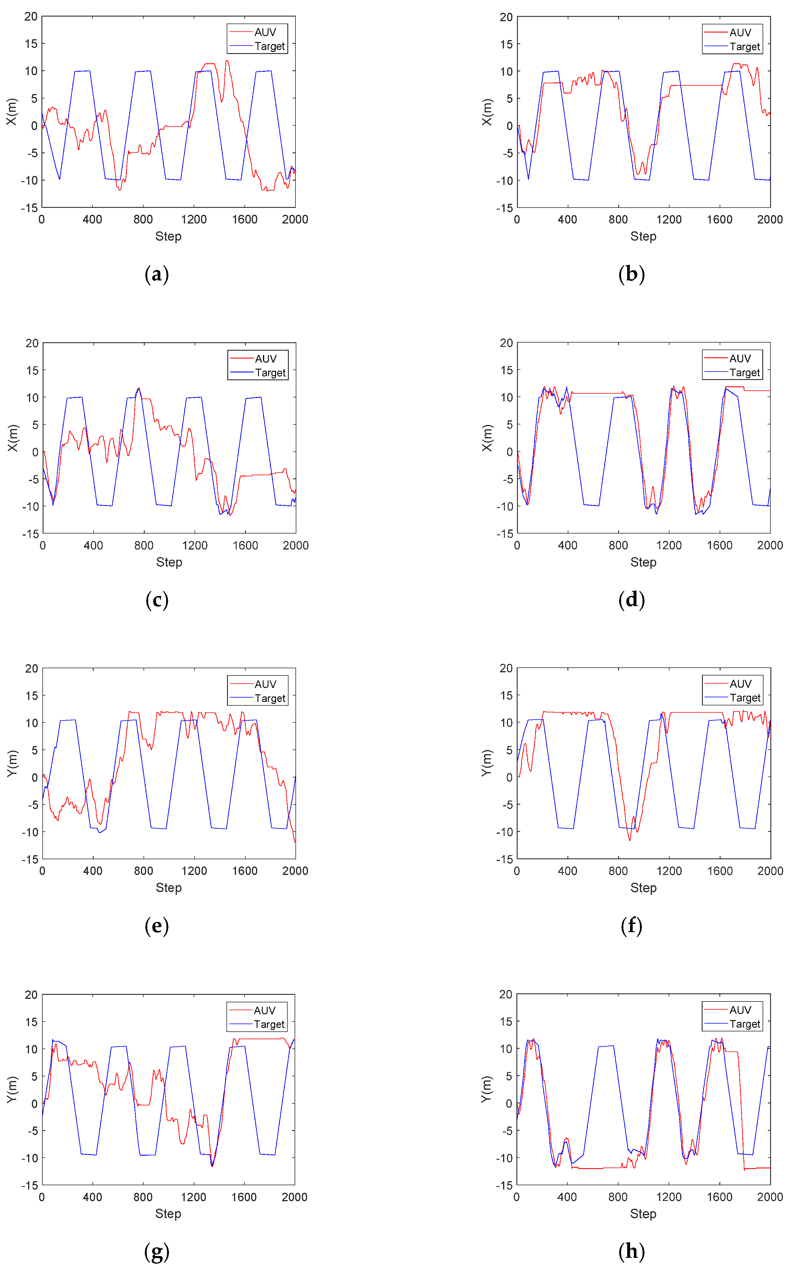
In Figure 6a,e, the AUV can effectively track the target using PPO during the 0–300 steps, but the Y-coordinate change of the AUV and the target have a large deviation after 300 steps, indicating that the AUV was unable to track the target during this period. Figure 6b,f shows that the distance between the AUV and the target is always kept at a small value throughout the tracking process except during the 1000–1300 steps. It shows that the training effect of SAC is better than that of PPO. As can be seen from Figure 6c,g, the trajectories of the AUV and the target are more similar using GAIL compared to SAC. In addition, in the whole tracking process, there is a large difference in the Y-coordinate during 1500–1600 steps only, indicating that the GAIL controller has a better tracking effect than SAC. It can be seen from Figure 6d,h that the AUV is always close to the target throughout the tracking process using the MAG controller. Therefore, the tracking accuracy of the MAG controller is the best among the four methods.

In Figure 7a,e, there is a big distance error between the AUV and the target using PPO during 1300–1400 steps only. Compared with the trajectory of the AUV and the target in Figure 6a,e, the tracking accuracy of the PPO controller is less affected by noise. Figure 7b,f shows that the AUV loses the target for more time in Scene 2 than in Scene 1, indicating that the tracking ability of the SAC controller deteriorated due to the noise. From the Figure 7c,d,g,h, it can be seen that the distance is smaller using PPO than GAIL during the whole tracking process. This shows that in Scene 2, both the GAIL and MAG controllers have better tracking accuracy, but compared with GAIL, the MAG controller can bring the AUV closer to the target. This indicates that the MAG controller has the best anti-interference.

Figure 8 shows the trajectory of the AUV and the target using four methods in Scene 3. It can be seen that the control effect of the four methods becomes significantly worse than in Scene 1. It shows that the AUV acts more cautiously when colliding with an obstacle is negatively rewarded. In Figure 8a,b,e,f, the AUV hesitated for a long time and went further and further away from the target when using PPO or SAC. When using the GAIL controller, the trajectory of the AUV and the target is quite different in the whole tracking process; it is considered that the AUV cannot complete the task of tracking the target. Compared with other methods, the MAG controller makes the AUV track the target for the longest time. The tracking effect is also better than that of the other three methods.

In order to verify that the proposed method still has good performance even when the number of training steps is reduced, we reduced the number of training steps to 20,000 times. We compared with the PPO and GAIL in Scenes 1 and 2 to simplify the experiment. Figure 9 shows that after the training times were reduced, the tracking accuracy of PPO and GAIL dropped significantly in Scenes 1 and 2, whereas the MAG controller could still enable the AUV to track the target, indicating that when the training times are low, the MAG controller already has good performance.

In

Table 4. Comparison of tracking performance after AUV training 20,000 times using PPO, GAIL, and MAG in Scenes 1 and 2.

	Scene 1			Scene 2
	PPO [48]	GAIL [51]	MAG (Ours)	PPO [48]	GAIL [51]	MAG (Ours)
$\stackrel{-}{d}$	12.8324	8.1974	1.4853	11.1855	7.1754	1.1321
$Va{r}_d$	6.2000	1.0495	0.7206	3.7951	0.7804	0.5229
$\stackrel{-}{x_a}$	4.0641	1.3391	5.6856	−7.7581	−2.3172	−6.1136
$\stackrel{-}{y_a}$	2.9278	−0.3948	7.8973	−0.2228	0.7792	7.9131
$\stackrel{-}{x_g}$	−1.0678	−0.8711	6.2315	−1.0512	−1.2140	−6.6929
$\stackrel{-}{y_g}$	2.4404	2.3525	7.8203	2.4347	1.5609	8.2772

, $(\stackrel{-}{x_a},\stackrel{-}{y_a})$ is the average value of the coordinates of the AUV, and $(\stackrel{-}{x_g},\stackrel{-}{y_g})$ is the average value of coordinates of the target. After the training time is reduced, from the perspective of distance, the tracking accuracy of MAG is better than that of PPO and GAIL, and the variance value is also smaller, indicating that the tracking process is smoother. From the perspective of coordinates, the coordinates of the AUV using the MAG are closer to the target, indicating that the MAG can train the optimal network earlier.

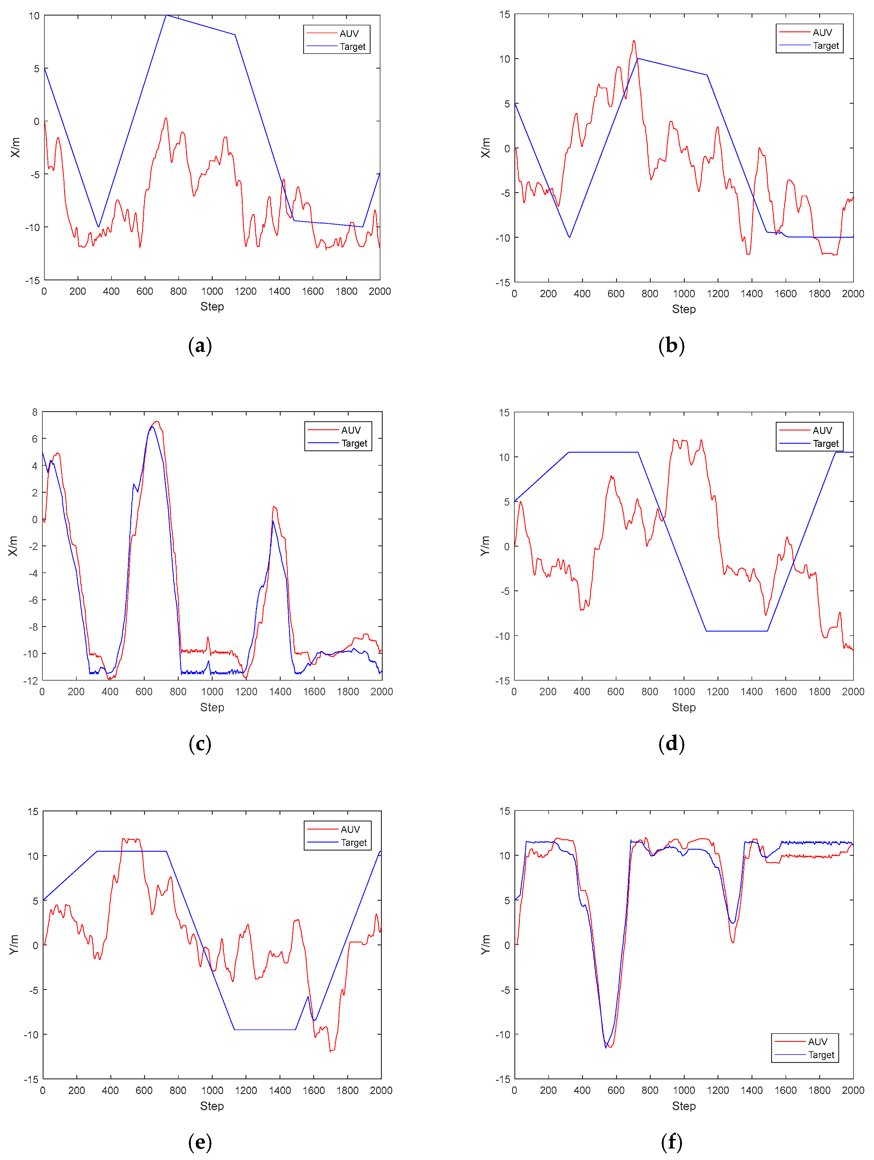
Figure 10 shows the movement trajectory of the AUV and the target during the process of the AUV tracking the target using the three methods in Scene 1. It can be seen from Figure 10a,d that if the distance becomes large, the tracking accuracy is poor. In Figure 10b,e, the distance decreased to a certain extent using GAIL, but the target still could not be tracked effectively. Figure 10c,f shows that the distance is the smallest, meaning that the task of tracking the target could be successfully completed, and the tracking effect is better, indicating that multi-agent training can improve the effect of network training.

Figure 11 shows the motion trajectory of the AUV and the target during the process of the AUV tracking the target using the three methods in Scene 2. Figure 11a,b,d,e shows that during the process of the AUV using PPO and GAIL to track the target, the AUV movement trajectory is very different from the target movement trajectory. On the other hand, Figure 11c,f indicates that during the process of the AUV tracking the target using MAG, the gap between the target motion trajectory and the AUV motion trajectory was small, and the tracking effect better. It shows that in the case of fewer training times, it is more efficient to add multi-agent training to train the AUV and accelerate the exploration.

5. Conclusions

This paper proposes a multi-agent training algorithm based on PPO combined with a GAN framework to control an AUV tracking a target. AUVs learn directly from expert demonstrations to solve the sparse reward problem. In addition, it avoids convergence by multi-agent training. Simulation experiments prove that when performing dynamic target-tracking tasks, this controller has better tracking accuracy than PPO, SAC, and GAIL. However, the starting point position and complexity of the environment have a certain impact on the performance of the underwater robot tracking the target. In the future, further improvements will be made to the proposed method to reduce the training time. The real simulation experiments are also very important to the actual motion control. Since the starting point of this paper is to verify the feasibility and effectiveness of the control algorithm, random noise interference and four obstacles were added to the plane environment. In the application to the actual underwater system, the change of hydrodynamic coefficients at different depths and other factors need to be considered.

References

1. Chen, Q. Unmanned Underwater Vehicle, 1st ed.; National Defense Industry Press: Beijing, China, 2014; pp. 1–27. [Google Scholar]
2. Kobayashi, R.; Okada, S. Development of hovering control system for an underwater vehicle to perform core internal inspections. J. Nucl. Sci. Technol. 2016, 53, 566–573. [Google Scholar] [CrossRef]
3. Li, Y.; Ma, T.; Wang, R.; Chen, P.; Zhang, Q. Terrain correlation correction method for AUV seabed terrain mapping. J. Navig. 2017, 70, 1062–1078. [Google Scholar] [CrossRef]
4. Zhao, Y.; Gao, F.; Yu, J.; Yu, X.; Yang, Z. Underwater image mosaic algorithm based on improved image registration. Appl. Sci. 2021, 11, 5986. [Google Scholar] [CrossRef]
5. Han, Y.; Liu, Y.; Hong, Z.; Zhang, Y.; Yang, S.; Wang, J. Sea ice image classification based on heterogeneous data fusion and deep learning. Remote Sens. 2021, 13, 592. [Google Scholar] [CrossRef]
6. Gao, F.; Wang, K.; Yang, Z.; Wang, Y.; Zhang, Q. Underwater image enhancement based on local contrast correction and multi-scale fusion. J. Mar. Sci. Eng. 2021, 9, 225. [Google Scholar] [CrossRef]
7. Conti, R.; Meli, E.; Ridolfi, A.; Allotta, B. An innovative decentralized strategy for I-AUVs cooperative manipulation tasks. Robot. Auton. Syst. 2015, 72, 261–276. [Google Scholar] [CrossRef]
8. Ribas, D.; Ridao, P.; Turetta, A.; Melchiorri, C.; Palli, G.; Fernández, J.J.; Sanz, P.J. I-AUV Mechatronics integration for the TRIDENT FP7 project. IEEE/ASME Trans. Mechatron. 2015, 20, 2583–2592. [Google Scholar] [CrossRef]
9. Mazumdar, A.; Triantafyllou, M.S.; Asada, H.H. Dynamic analysis and design of spheroidal underwater robots for precision multidirectional maneuvering. IEEE/ASME Trans. Mechatron. 2015, 20, 2890–2902. [Google Scholar] [CrossRef]
10. Ang, K.H.; Chong, G.; Li, Y. PID control system analysis, design, and technology. IEEE Trans. Control Syst. Technol. 2005, 13, 559–576. [Google Scholar]
11. Balogun, O.; Hubbard, M.; DeVries, J. Automatic control of canal flow using linear quadratic regulator theory. J. Hydraul. Eng. 1988, 114, 75–102. [Google Scholar] [CrossRef]
12. Li, S.; Liu, J.; Xu, H.; Zhao, H.; Wang, Y. Research status of my country’s deep-sea autonomous underwater vehicles. SCIENTIA SINICA Inf. 2018, 48, 1152–1164. [Google Scholar] [CrossRef] [Green Version]
13. Malinowski, M.; Kazmierkowski, M.P.; Trzynadlowski, A.M. A comparative study of control techniques for PWM rectifiers in AC adjustable speed drives. IEEE Trans. Power Electron. 2003, 18, 1390–1396. [Google Scholar] [CrossRef]
14. Christudas, F.; Dhanraj, A.V. System identification using long short term memory recurrent neural networks for real time conical tank system. Rom. J. Inf. Sci. Technol. 2020, 23, 57–77. [Google Scholar]
15. Zamfirache, I.A.; Precup, R.-E.; Roman, R.-C.; Petriu, E.M. Reinforcement Learning-based control using Q-learning and gravitational search algorithm with experimental validation on a nonlinear servo system. Inf. Sci. 2022, 583, 99–120. [Google Scholar] [CrossRef]
16. Precup, R.-E.; Roman, R.-C.; Teban, T.-A.; Albu, A.; Petriu, E.M.; Pozna, C. Model-free control of finger dynamics in prosthetic hand myoelectric-based control systems. Stud. Inform. Control 2020, 29, 399–410. [Google Scholar] [CrossRef]
17. Precup, R.-E.; Roman, R.-C.; Safaei, A. Data-Driven Model-Free Controllers, 1st ed.; CRC Press: Boca Raton, FL, USA, 2021; pp. 167–210. [Google Scholar]
18. Nian, R.; Liu, J.; Huang, B. A review on reinforcement learning: Introduction and applications in industrial process control. Comput. Chem. Eng. 2020, 139, 106886. [Google Scholar] [CrossRef]
19. Webb, G.I.; Pazzani, M.J.; Billsus, D. Machine learning for user modeling. User Modeling User-Adapt. Interact. 2001, 11, 19–29. [Google Scholar] [CrossRef]
20. Whitehead, S. Reinforcement Learning for the Adaptive Control of Perception and Action. PhD Thesis, University of Rochester, New York, NY, USA, 1992. [Google Scholar]
21. Tariq, M.I.; Tayyaba, S.; Ashraf, M.W.; Balas, V.E. Deep learning techniques for optimizing medical big data. In Deep Learning Techniques for Biomedical and Health Informatics, 1st ed.; Agarwal, B., Balas, V., Jain, L., Poonia, R., Sharma, M., Eds.; Academic Press: New York, NY, USA, 2020; pp. 187–211. [Google Scholar]
22. Ghasrodashti, E.K.; Sharma, N. Hyperspectral image classification using an extended Auto-Encoder method. Signal Processing Image Commun. 2021, 92, 116111. [Google Scholar] [CrossRef]
23. Wang, D.; Cao, W.; Zhang, F.; Li, Z.; Xu, S.; Wu, X. A review of deep learning in multiscale agricultural sensing. Remote Sens. 2022, 14, 559. [Google Scholar] [CrossRef]
24. Watkins, C.J.; Dayan, P. Q-learning. Mach. Learn. 1992, 8, 279–292. [Google Scholar] [CrossRef]
25. Ishii, K.; Fujii, T.; Ura, T. An on-line adaptation method in a neural network based control system for AUVs. IEEE J. Ocean. Eng. 1995, 20, 221–228. [Google Scholar] [CrossRef]
26. Schulman, J.; Wolski, F.; Dhariwal, P.; Radford, A.; Klimov, O. Proximal policy optimization algorithms. arXiv 2017, arXiv:1707.06347. [Google Scholar]
27. Haarnoja, T.; Zhou, A.; Abbeel, P.; Levine, S. Soft actor-critic: Off-policy maximum entropy deep reinforcement learning with a stochastic actor. In Proceedings of the 35th International Conference on Machine Learning, Stockholm, Sweden, 10–15 July 2018; pp. 1861–1870. [Google Scholar]
28. Yang, W.; Bai, C.; Cai, C. Survey on sparse reward in deep reinforcement learning. Comput. Sci. 2020, 47, 182–191. [Google Scholar]
29. Wan, L.; Lan, X.; Zhang, H.; Zheng, N. Survey on deep reinforcement learning theory and its application. Pattem. Recognit. Aitificial Intell. 2019, 32, 67–81. [Google Scholar]
30. Osa, T.; Sugita, N.; Mitsuishi, M. Online trajectory planning and force control for automation of surgical tasks. IEEE Trans. Autom. Sci. Eng. 2017, 15, 675–691. [Google Scholar] [CrossRef]
31. Sermanet, P.; Xu, K.; Levine, S. Unsupervised perceptual rewards for imitation learning. arXiv 2016, arXiv:1612.06699. [Google Scholar]
32. Torabi, F.; Warnell, G.; Stone, P. Behavioral cloning from observation. arXiv 2018, arXiv:1805.01954. [Google Scholar]
33. Ng, A.Y.; Russell, S.J. Algorithms for inverse reinforcement learning. In Proceedings of the 17th International Conference on Machine Learning, Vienna, Austria, 12–18 July 2000; pp. 663–670. [Google Scholar]
34. Ho, J.; Ermon, S. Generative adversarial imitation learning. In Proceedings of the 30th International Conference on Neural Information Processing Systems, Barcelona, Spain, 5–10 December 2016; pp. 4565–4573. [Google Scholar]
35. Riedmiller, M. Neural fitted Q iteration–first experiences with a data efficient neural reinforcement learning method. In Proceedings of the 16th European Conference on Machine Learning, Porto, Portugal, 3–7 October 2005; pp. 317–328. [Google Scholar]
36. Gupta, J.K.; Egorov, M.; Kochenderfer, M. Cooperative multi-agent control using deep reinforcement learning. In Proceedings of the International Conference on Autonomous Agents and Multiagent Systems, Sao Paulo, Brazil, 8–12 May 2017; pp. 66–83. [Google Scholar]
37. Babaeizadeh, M.; Frosio, I.; Tyree, S.; Clemons, J.; Kautz, J. Reinforcement learning through asynchronous advantage actor-critic on a gpu. arXiv 2016, arXiv:1611.06256. [Google Scholar]
38. Fossen, T.I. Handbook of Marine Craft Hydrodynamics and Motion Control, 2nd ed.; John Wiley & Sons: West Sussex, UK, 2021; pp. 3–14. [Google Scholar]
39. Wang, Z.; Merel, J.S.; Reed, S.E.; de Freitas, N.; Wayne, G.; Heess, N. Robust imitation of diverse behaviors. In Proceedings of the 31st International Conference on Neural Information Processing Systems, Long Beach, CA, USA, 4–9 December 2017; pp. 5320–5329. [Google Scholar]
40. Vanvuchelen, N.; Gijsbrechts, J.; Boute, R. Use of proximal policy optimization for the joint replenishment problem. Comput. Ind. 2020, 119, 103239. [Google Scholar] [CrossRef]
41. Yu, X.; Sun, Y.; Wang, X.; Zhang, G. End-to-end AUV motion planning method based on soft actor-critic. Sensors 2021, 21, 5893. [Google Scholar] [CrossRef]
42. Choi, S.; Kim, J.; Yeo, H. Trajgail: Generating urban vehicle trajectories using generative adversarial imitation learning. Transp. Res. Part C Emerg. Technol. 2021, 128, 103091. [Google Scholar] [CrossRef]
43. Herlambang, T.; Djatmiko, E.B.; Nurhadi, H. Ensemble Kalman filter with a square root scheme (EnKF-SR) for trajectory estimation of AUV SEGOROGENI ITS. Int. Rev. Mech. Eng. 2015, 9, 553–560. [Google Scholar] [CrossRef]
44. Yuan, J.; Wang, H.; Zhang, H.; Lin, C.; Yu, D.; Li, C. AUV obstacle avoidance planning based on deep reinforcement learning. J. Mar. Sci. Eng. 2021, 9, 1166. [Google Scholar] [CrossRef]
45. Ganesan, V.; Chitre, M.; Brekke, E. Robust underwater obstacle detection and collision avoidance. Auton. Robot. 2016, 40, 1165–1185. [Google Scholar] [CrossRef]
46. You, X.; Lv, Z.; Ding, Y.; Su, W.; Xiao, L. Reinforcement learning based energy efficient underwater localization. In Proceedings of the 2020 International Conference on Wireless Communications and Signal Processing (WCSP), Wuhan, China, 21–23 October 2020; pp. 927–932. [Google Scholar]
47. MahmoudZadeh, S.; Powers, D.; Yazdani, A.M.; Sammut, K.; Atyabi, A. Efficient AUV path planning in time-variant underwater environment using differential evolution algorithm. J. Mar. Sci. Appl. 2018, 17, 585–591. [Google Scholar] [CrossRef]
48. Bøhn, E.; Coates, E.M.; Moe, S.; Johansen, T.A. Deep reinforcement learning attitude control of fixed-wing uavs using proximal policy optimization. In Proceedings of the 2019 International Conference on Unmanned Aircraft Systems (ICUAS), Atlanta, GA, USA, 11–14 June 2019; pp. 523–533. [Google Scholar]
49. Barros, G.M.; Colombini, E.L. Using soft actor-critic for low-level UAV control. arXiv 2020, arXiv:2010.02293. [Google Scholar]
50. Grando, R.B.; de Jesus, J.C.; Kich, V.A.; Kolling, A.H.; Bortoluzzi, N.P.; Pinheiro, P.M.; Neto, A.A.; Drews, P.L. Deep reinforcement learning for mapless navigation of a hybrid aerial underwater vehicle with medium transition. In Proceedings of the 2021 IEEE International Conference on Robotics and Automation (ICRA), Xi’an, China, 30 May–5 June 2021; pp. 1088–1094. [Google Scholar]
51. Pham, D.-T.; Tran, T.-N.; Alam, S.; Duong, V.N. A generative adversarial imitation learning approach for realistic aircraft taxi-speed modeling. IEEE Trans. Intell. Transp. Syst. 2021, in press. [Google Scholar] [CrossRef]
52. Tai, L.; Zhang, J.; Liu, M.; Burgard, W. Socially compliant navigation through raw depth inputs with generative adversarial imitation learning. In Proceedings of the 2018 IEEE International Conference on Robotics and Automation (ICRA), Brisbane, Australia, 21–26 May 2018; pp. 1111–1117. [Google Scholar]
Figure 1. Inertial coordinate system and motion coordinate system of AUV.
Jmse 10 00383 g001
Figure 2. AUV tracking target diagram.
Jmse 10 00383 g002
Figure 3. Structure diagram of MAG algorithm.
Jmse 10 00383 g003
Figure 4. The reward obtained by the AUV using four methods in Scenes 1, 2, and 3: (a) Scene 1; (b) Scene 2; and (c) Scene 3.
Jmse 10 00383 g004
Figure 5. Real-Time distance between the AUV and target training 100,000 times in Scenes 1 and 2: (a) Scene 1 and (b) Scene 2.
Jmse 10 00383 g005
Figure 6. The coordinate change curves in Scene 1 during the process of AUV tracking the target using PPO, SAC, GAIL, and MAG, respectively: (ad) the X-coordinate change; (eh) the Y-coordinate change.
Jmse 10 00383 g006aJmse 10 00383 g006b
Figure 7. The coordinate change curves in Scene 2 during the process of AUV tracking the target using PPO, SAC, GAIL, and MAG, respectively: (ad) the X-coordinate change; (eh) the Y-coordinate change.
Jmse 10 00383 g007aJmse 10 00383 g007b
Figure 8. The coordinate change curves in Scene 3 during the process of AUV tracking the target using PPO, SAC, GAIL, and MAG, respectively: (ad) the X-coordinate change; and (eh) the Y-coordinate change.
Jmse 10 00383 g008
Figure 9. Real-Time distance between the AUV and target training 20,000 times in Scenes 1 and 2: (a) in Scene 1 and (b) in Scene 2.
Jmse 10 00383 g009
Figure 10. The coordinate change curves during the process of AUV tracking the target using PPO, GAIL, and MAG, respectively, training 20,000 times in Scene 1: (ac) the X-coordinate change; and (df) the Y-coordinate change.
Jmse 10 00383 g010
Figure 11. The coordinate change curves during the process of AUV tracking the target using PPO, GAIL, and MAG, respectively, training 20,000 times in scene 2: (a–c) the X-coordinate change; and (df) the Y-coordinate change.
Jmse 10 00383 g011