Stabilization of Neural Network Models for VIV Force Data Using Decoupled, Linear Feedback

Abstract

The hydrodynamic forces on an oscillating circular cylinder are predicted using neural networks under flow conditions where Vortex-Induced Vibrations (VIV) are known to occur. The derived neural network approximators are then incorporated in a dynamical model that allows prediction of the cylinder motion given flow conditions and initial conditions. Using experimental data, a minimum-least-squares compensator is tuned that includes linear stiffness and damping su-perimposed with a constant force offset. The compensator is decoupled, i.e., with equations in-dependent for each degree of freedom. By applying the neural network approximators and the derived compensator simulated experiments can be performed. These simulated experiments show that the compensator which cancels the linear components and any bias in the hydrody-namic forces effectively stabilizes the VIV motion. To support this time-domain analysis is per-formed along with phase-plane investigations. Maximum Lyapunov exponent analysis is also shown.

1. Introduction

In many engineering applications, vortex-induced vibrations (VIV) constitute a dynamic, non-linear fluid–structure interaction (e.g., offshore structures, towed cables, mooring systems, ship appendages, buildings, bridges, power wires, pipelines, antennae, heat exchangers, etc.). This phenomenon has been widely observed, with multiple reviews devoted to the subject and extensive literature review about one and two degree of freedom VIV can be found within these articles [1,2,3,4,5,6]. Vortices occur in the wake of a bluff object, such as a round cylinder, when fluid flows across it. When the shedding frequency of these vortices approaches the natural frequency of the structure, significant amplitude movements occur, which push the structure to vibrate more, resulting in a changed wake that forces the structure differently, and so on if the item is flexible or elastically attached. The acceleration of the surrounding dense fluid, such as water, adds greatly to the time-varying frequency properties of the vibrations, resulting in wide-band, large-amplitude vibrations. The prediction of these vibrations is crucial in thin ocean structure applications, notably for towing cables, risers, floating structures, and mooring systems, to minimize structural failure, wear, noise generation, and operational downtime.

New renewable offshore technologies, such as floating offshore wind turbines and in-stream energy, are being developed. Therefore, the phenomena has lately been extended as a possible energy production strategy [7]. The vibration of elastically placed circular cylinders in a current that are confined to cross-flow motion or motion perpendicular to the direction of the current has received a lot of attention in energy harvesting applications. Allowing the cylinder to move with mixed in-line and cross-flow motion relative to the direction of the fluid has the capacity to boost the amplitude responsiveness of the system, improving power output, in order to improve power output in energy harvesting. As a result, in order to create control techniques for VIV-based energy harvesters, dynamical models that can anticipate the forcing and behavior of this sort of system are required.

Previous research has shown that combining in-line and cross-flow motion improves both the cross-flow amplitude response and the lift direction harmonic forcing of a circular cylinder experiencing VIV [8,9]. Because of the greater amplitude vibrations, this can cause to increase fatigue in structures subjected to this fluid–structure interaction in standard designed systems [10]; however, in energy harvesting systems, these larger amplitude motions can be regulated to maximize energy harvesting capabilities. These larger amplitude vibrations might, however, be controlled in energy harvesting devices to boost energy gathering potential. It is challenging to construct simple fluid force models that can anticipate the fluid–structure coupling because the connection between motion and fluid forces is related non-linearly through the time-dependent shedding of vortices. When used with a structural model, semi-empirical approaches have enhanced efforts for modeling fluid forces by employing empirically-generated data from free vibration or forced motion studies to predict fluid forces.

Due to the direct use of real measured forces in the coupling prediction, semi-empirical prediction approaches that apply simple structural models mixed with an empirical database acquired from forced motion experiments have been found to be better predictors of cross-flow motion VIV [11,12,13,14]. However, extending these semi-empirical methods to include combined cross-flow and in-line motion can be difficult due to the large number of experiments required to generate a well-resolved database of force measurements, as in-line motion significantly increases the number of variables describing body motion. This semi-empirical approach was created to improve prediction skills in energy harvesting applications [15], but it has not yet been applied to systems that have both in-line and cross-flow motion. Furthermore, time-varying hydrodynamic coefficient models have been investigated in order to predict VIV in these types of applications [16,17].

Previous forced motion experiments investigating combined in-line and cross-flow motion over a sparse parameter space, including variations in cross-flow amplitude, in-line amplitude, reduced velocity, and phase between in-line and cross-flow motion, have not yet been successfully implemented in predictive tools for VIV [18]. This dataset has been extended to study the use of the dataset for semi-empirical prediction by resolving the lower amplitude parameter space. However, these investigations have resulted in a restricted examination of the resulting forces from combined in-line and cross-flow motions [19]. The use of a unique automated experimental apparatus to construct a database of forced combined in-line and cross-flow motions at a specific Reynolds number has resulted in a more resolved database [20,21,22], providing a rich source of hydrodynamic force data that can be used to develop artificial intelligence-based predictive force models.

In summary, references [1,2,3,4,5,6] provide a thorough account of VIV in one and two di-mensions while [7] explores the energy production potential of VIV. To expand on this potential, [8,9] investigate the coupling dynamics, while [10] investigates the impact of VIV on structures. Various approaches of phenomenological modeling of VIV are de-veloped in [11,12,13,14,15,16,17]. Finally, [18,19,20,21,22] define the requirements of data gathering cam-paigns toward development of VIV models. In this end, as part of our present study, we are going to use a comprehensive force database [20] to develop decoupled feed-back systems for stabilization of neural network models of one dimensional (1D) and two dimensional (2D) VIV force data. Previously, Artificial Neural Network force models were built based on several tests in order to provide a time-dependent forecast of the force on the body based on position and velocity inputs [23]. In order to improve the neural network model using autoregressive techniques, an error estimation model was constructed for the existing neural network hydrodynamic force model. The time dependent neural network prediction model was improved as a result of this [24]. We are going to develop a decoupled, linear feedback system which is used to stabilize neural network models of VIV force data. In order to achieve this, we are going to use one neural network model from our in-house database to show how the dynamics of the entire system work.

2. Methods and Applications

2.1. Experimental Details

In the experimental fluid mechanics laboratory at the University of Rhode Island (URI), automated forced two-degree-of-freedom experiments were carried out. Figure 1 depicts the experiment setup. A towing tank, automated linear actuators, a control box, and a data acquisition (DAQ) system make up the experiment setup. A 4.3 m by 0.9 m by 0.8 m glass tank with tow carriage serves as motion control tank. The tow carriage is fitted with an X–Y linear actuator system as well as a Z rotational motor. A six-axis force sensor placed on the tow point provides force measurement. The system is entirely automated thanks to a MATLAB control interface between control box and DAQ system that allows for automated experiment control by control box based on the decision-making algorithm. A primary carriage is mounted on top of the water tank and can travel with constant speed. Linear actuators conduct prescribed figure-eight and crescent driven motions of a text cylinder attached to the carriage. While combined cross-flow and in-line VIV often results in figure-eight and crescent-shaped cylinder motions in a carriage-fixed reference frame, the nonlinear interaction of the structural system with the fluid does not guarantee that the motions are sinusoidal in each direction. For simplicity, the motion of the body is assumed to be sinusoidal for both cross-flow and in-line directions [25], such that these motions are only characterized by a single amplitude and single frequency. In addition, in-line motions are assumed to have double the frequency of cross-flow motions allowing for a single frequency parameter to represent the circular cylinder’s motion. This reduces the number of variables to consider while defining cylinder motion. Thus, forced motions are defined as

$$y\left(t\right)=A_{y}sin\left(\omega t\right)$$

(1)

$$x\left(t\right)=A_{x}sin\left(2\omega t+\theta \right)$$

(2)

The orbital motion of the cylinder in the carriage fixed reference frame is defined by the phase difference between in-line and cross-flow motions, $\theta$. Based on the non-dimensional amplitudes, the cylinder’s motion can be characterized non-dimensionally for both direction; non dimensional cross flow motion amplitude, $A_y/D$, non dimensional in-line motion amplitude, $A_x/D$ and also a single cross-flow reduced velocity can be defined based on carriage speed, motion frequency and the diameter of cylinder:

$$V_r=\frac{U2\pi }{\omega D}$$

(3)

The in-line amplitude was varied from 0.1 to 0.5 in increments of 0.1, the cross-flow amplitude from 0.1 to 1.6 in increments of 0.25, the non-dimensional speed parameter, the reduced velocity from 4 to 8 in increments of 0.2, and the phase between in-line and cross-flow motions from −180 degrees to 180 degrees in increments of 30 degrees. As a result, the experimental database for the single Reynolds number of 7620 has 9555 ex-periments. Each run was carried out using an automated system, which ensured that the experiment was always reset to the same starting point and that the following ex-periment was carried out after an interval of 8.5 minutes. ATI Gamma SI-65-10 and SI-130-10 six-axis force sensors were used to measure hydrodynamic forces.

The lift and drag forces, $F_y$ and $F_x$, can be approximated as sinusoidal functions with dominant frequencies equal to the motion frequencies up to first order:

$$F_y=F_1\sin \left(\omega t+{\varphi }_1\right)$$

(4)

$$F_x=F_2\sin \left(2\omega t+{\varphi }_2\right)$$

(5)

The phase angles between motion and force are ${\varphi }_1$ and ${\varphi }_2$ respectively according to the equation. Depending on the sign of the power transfer, the component of the force in phase with the velocity of the cylinder motion may either excite or dampen the motion of a freely vibrating system. This power transfer is a function of forces in both lift and drag for a system oscillating with combined in-line and cross-flow motion. The power is normalized to obtain an average power coefficient, $C_{ap}$, that represents the excitation of the structure. A system with a positive power coefficient has net energy transmitted from the fluid to the body, indicating positive structure excitation. A freely vibrating system may experience this form of motion. A negative power coefficient implies a net energy transfer from the structure to the fluid, which occurs exclusively in forced motions. As a result, we may define an average power transfer coefficientas follows: Positive power transfer denotes excitation and energy transfer from the fluid to the body, whereas negative power transfer denotes damping and energy transfer from the body to the fluid:

$$C_{ap}=\frac{\frac{1}{T}{{\displaystyle \int }}_0^T\left(F_y·\dot{y}+F_x·\dot{x}\right)dt}{\frac{1}{2}\rho U^{3}DL}$$

(6)

Varying in cross-flow motion amplitude and reduced velocity for fixed phase between in-line and cross-flow motion are shown in Figure 2 on contour plots to show the average power coefficient for fixed phase between in-line and cross-flow motion,$\theta =0^{°},$ and $A_x/D=0.1$ for fixed in-line amplitude. The white region where the average power coefficient is positive represents the free vibration region. In prior work, cylinder movements corresponding to this free vibration zone were used to generate the predicted force model using neural nets. Based on the full measured forces, 26 experimental runs were chosen for creating neural network estimators for lift force and a drag force [23,24].

2.2. Feedback Stabilization

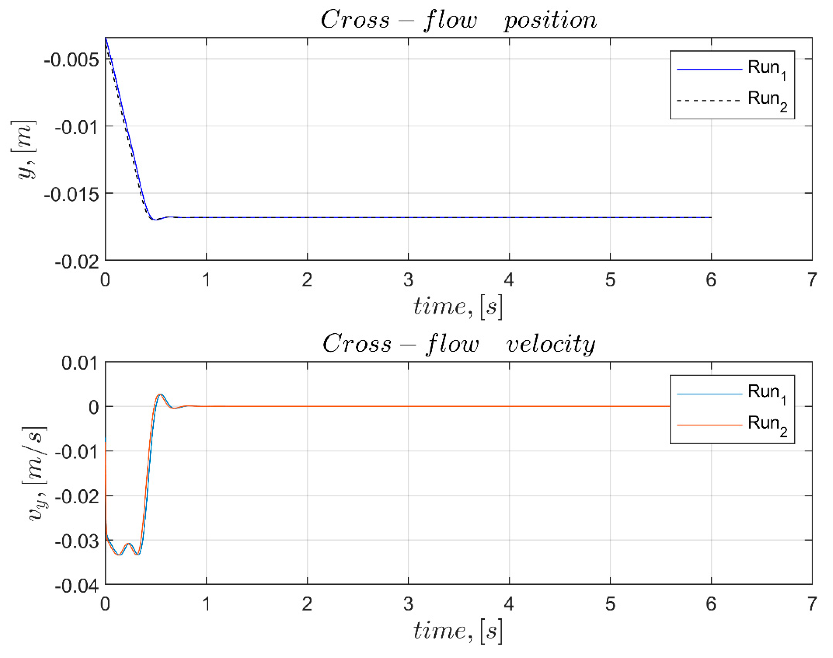
A decoupled, linear feedback law is used to stabilize the dynamics of VIV motion with neural network approximators for the hydrodynamic forces driving the process. The time series of lift and drag forces were previously approximated using Artificial Neural Networks (ANN) with position and velocity signals as inputs and lift and drag force time series as output. A feedforward ANN is used to create nonlinear force approximators from experimental data sets. The ANN is a closed form mathematical equation, with weights defined by the ANN’s training. [23,24,26,27]. The cylinder motions (in-line and cross-flow position and velocity) are defined as inputs to the ANN model, while the force time series in x and y are defined as outputs:

$${\widehat{\mathit{F}}}_{\mathit{n}}\equiv \widehat{\mathit{F}}\left(\mathit{t}=\mathit{n}{\mathit{T}}_{\mathit{s}}\right)=\mathit{f}\left(\overrightarrow{\mathit{a}}\right)$$

(7)

$$\overrightarrow{\mathit{a}}={\left[\mathit{x} \mathit{y} \dot{\mathit{x}} \dot{\mathit{y}}\right]}^T$$

(8)

a is the input vector with position and velocity for in-line and cross-flow motions, and $\widehat{\mathit{F}}$ is the force estimates from the ANN. The sampling time is ${\mathit{T}}_{\mathit{s}}$ = 0.001 s, as determined by the tank measurements in the experimental database, F.

A total of 52 neural nets were trained as part of past work to encompass the results of 26 forced vibration experiments. For each experiment, one neural network was trained as approximator of time-dependent lift and one net for drag force. The neural nets for lift and drag forces have a three-layer structure. Feedforward systems, such as neural nets, require an input vector as well as hidden and output layers. The input and output layers of all 52 nets are both linear. Each neural net of the 52 ones has four input variables: The instantaneous position in cross-flow direction, instantaneous position in in-line direction, instantaneous velocity in cross-flow direction, and instantaneous velocity in in-line direction. Each input was transmitted to the hidden layer by a dedicated neuron in the input layer. The 26 lift force neural approximators have 7 neurons in the hidden layer. The 26 drag force neural approximators have 11 neurons in the hidden layer. MATLAB’s neural network toolbox was used to create all 52 ANNs. The transfer function (also known as activation function) of all nodes in the hidden layers of all 52 nets was the nonlinear tangent sigmoid, while the output layer, as previously stated, was linear. Because the sampling rate of the experiments was quite high, the experimental data have good temporal resolution, with a significant number of data points for each run.

In conclusion, for the lift and drag force, the approximator $\widehat{\mathit{F}}$ has the following form.

$$\widehat{\mathit{F}}={\mathit{W}}_0·\overrightarrow{\mathit{g}}\left(\mathit{W}·\overrightarrow{\mathit{a}}+\overrightarrow{\mathit{b}}\right)+{\mathit{b}}_0$$

(9)

where W is the hidden weight values matrix, a is a vector holding the input values, b is the hidden bias values column vector, ${\mathit{W}}_0$ is the row vector encompassing output weight values and ${\mathit{b}}_0$ is the output bias value. Finally, $\overrightarrow{\mathit{g}}$ is a column vector with the same dimension as vector $\left(\mathit{W}·\overrightarrow{\mathit{a}}+\overrightarrow{\mathit{b}}\right)$; $\overrightarrow{\mathit{g}}$ is holding the values the activation function assumes when applied to each scalar component of vector $\left(\mathit{W}·\overrightarrow{\mathit{a}}+\overrightarrow{\mathit{b}}\right)$. In our case, the activation function is the tangent sigmoid function (tanh) defined as follows.

$$\mathit{g}\left(\mathit{\chi }\right)=\mathbf{tanh}\left(\mathit{\chi }\right)=\frac{{\mathit{e}}^{\mathit{\chi }}-{\mathit{e}}^{-\mathit{\chi }}}{{\mathit{e}}^{\mathit{\chi }}+{\mathit{e}}^{-\mathit{\chi }}}=\frac{\mathbf{1}-{\mathit{e}}^{-\mathbf{2}\mathit{\chi }}}{\mathbf{1}+{\mathit{e}}^{-\mathbf{2}\mathit{\chi }}}=\frac{\mathbf{2}}{\mathbf{1}+{\mathit{e}}^{-\mathbf{2}\mathit{\chi }}}-\mathbf{1}$$

(10)

To avoid overtraining, for each experimental run, 40% of the data points in the recorded time history were chosen at random to be utilized as training data for calibrating the weights and biases of the net. The maximum number of epochs allowed for training the nets was 1000. The training of the neural nets was completed at a specific epoch number when the best validation performance was achieved based on the mean squared error. The number of epochs required for the lift force neural nets to meet the training objective of mean square error less or equal to 0.015 was about 120; for the drag force neural nets, the number of epochs to meet the training objective of mean square error less or equal to 0.00145 was about 250, 40% of data points were used to train the ANN model. In this paper, we are using the neural network approximators for lift and drag force from a single certain experiment to investigate stabilization of the dynamics using decoupled linear feedback as explained in the methodology below. The weight and bias values obtained after training the neural nets toward lift force and drag force approximation for the typical case examined in the remainder of this text are shown in the Appendix A.

The starting point is the equations of motion, which will be employed in virtual (i.e., simulated) experiments of the two degree of freedom system at hand. The cross-flow (lift) direction is represented by the y axis, while the in-line (drag) direction is represented by the x axis.

$${\mathit{f}}_{\mathit{y}}+\mathit{m}\ddot{\mathit{y}}+{\mathit{b}}_{\mathit{y}}\dot{\mathit{y}}+{\mathit{k}}_{\mathit{y}}\mathit{y}={\widehat{\mathit{F}}}_{\mathit{y}}$$

(11)

$${\mathit{f}}_{\mathit{x}}+\mathit{m}\ddot{\mathit{x}}+{\mathit{b}}_{\mathit{x}}\dot{\mathit{x}}+{\mathit{k}}_{\mathit{x}}\mathit{x}={\widehat{\mathit{F}}}_{\mathit{x}}$$

(12)

In the above, $\mathit{m}$ is the structural mass of the oscillating body in the experiments and equal to 0.268 kg, ${\mathit{f}}_{\mathit{y}}$ and ${\mathit{f}}_{\mathit{x}}$ are constant offset forces along the lift and drag direction, respectively (since per the experiment the hydrodynamic forces were generally biased, i.e., not zero mean); cross-flow and in-line direction structural damping coefficients are represented by ${\mathit{b}}_{\mathit{y}}$ and ${\mathit{b}}_{\mathit{x}}$, respectively. The cross-flow and drag direction spring constants are ${\mathit{k}}_{\mathit{y}}$ and ${\mathit{k}}_{\mathit{x}}$, respectively. First, system parameters such as structural damping, stiffness coefficients, and force offsets are found based on minimum least-squares optimization method, shown in

Table 1. Optimized system parameters.

	k (N/m)	b (kg/s)	Offset Force, f (N)
y	186.01	9.25	0.007
x	188.84	−0.35	0.72

, in order to develop a dynamical simulation model to predict position and velocity from the equations of motion above.

These system parameters are used in the dynamical simulation models developed for the oscillating body’s position and velocity. Two distinct cases are investigated in form of virtual (i.e., simulated on computer) experiments: full 2D case and 1D case with motion along the x-axis suppressed. In order to check stability, the Lyapunov exponent is calculated for each simulation. Given some initial variables, $a_0$, we consider a neighboring point,$a_0+\delta Z_0$, with distance $\delta Z_0$ sufficiently small. We assume that $\delta Z_N$ is going to be the distance after N iterations. Therefore, $|\delta Z_N\left|\approx |\delta Z_0\right|e^{\lambda N\delta t}$ and $\lambda$ is called (maximum) Lyapunov exponent. A signature of chaos is a positive Lyapunov exponent [28,29]. The maximum Lyapunov exponent can be estimated as follows by performing two runs starting from random yet sufficiently close initial conditions and iterating the dynamical model N times

$$\lambda =\underset{N\to \infty }{\lim }\frac{1}{N \delta t}\ln \left|\frac{\delta Z_N}{\delta Z_0}\right|$$

(13)

We first describe the procedure for the 2D (i.e., both lift and drag directions considered) simulated experiment since it is more general. The dynamics along the x-axis and y-axis for each one of these simulated experiments are governed by the following equations of motion.

$$\ddot{y}=\frac{{\widehat{F}}_y-b_y\dot{y}-k_{y}y-f_y}{m}$$

(14)

$$\ddot{x}=\frac{{\widehat{F}}_x-b_x\dot{x}-k_{x}x-f_x}{m}$$

(15)

where $f_x$ and $f_y$ are the force offsets and m is the mass of the cylinder equal to 0.268 kg. After acceleration is calculated for each time step, as shown in Figure 3, velocity and position are generated using numerical integration twice with sufficiently small time step.

For each simulated experiment, two runs, Run1 and Run2, are performed starting from neighboring initial conditions. For Run1, the initial conditions for position and velocity along the x- and y-axis are the measured values at a randomly selected point in time from the time series collected during experiments. For Run2, the initial conditions are a random perturbation of those in Run1; specifically

$${\left[\begin{array}{c}\begin{array}{c}x\left(t=0\right)\\ y\left(t=0\right)\end{array}\\ \begin{array}{c}\dot{x}\left(t=0\right)\\ \dot{y}\left(t=0\right)\end{array}\end{array}\right]}_{Run2}-{\left[\begin{array}{c}\begin{array}{c}x\left(t=0\right)\\ y\left(t=0\right)\end{array}\\ \begin{array}{c}\dot{x}\left(t=0\right)\\ \dot{y}\left(t=0\right)\end{array}\end{array}\right]}_{Run1}=\mathrm{diag}\left({\epsilon }_1, {\epsilon }_2,{\epsilon }_3,{\epsilon }_4\right){\left[\begin{array}{c}\begin{array}{c}x\left(0\right)\\ y\left(0\right)\end{array}\\ \begin{array}{c}\dot{x}\left(0\right)\\ \dot{y}\left(0\right)\end{array}\end{array}\right]}_{Run1}$$

(16)

In the above, factors ${\epsilon }_1,\dots ,{\epsilon }_4$ on the main diagonal of the diagonal matrix on the right-hand side are independent random variables following the Normal (Gaussian) Distribution with zero mean and standard deviation equal to 5% (i.e., 1/20).

For the 1D simulated experiments only the lift direction was considered. Initial conditions for the y-axis position and velocity were chosen randomly from the measurements, same as in the 2D case described above, but for the x-axis they were set to zero. In order to investigate stability, each simulated experiment consists of two runs with neighboring initial conditions related as follows.

$${\left[\begin{array}{c}\begin{array}{c}x\left(t=0\right)\\ y\left(t=0\right)\end{array}\\ \begin{array}{c}\dot{x}\left(t=0\right)\\ \dot{y}\left(t=0\right)\end{array}\end{array}\right]}_{Run2}-{\left[\begin{array}{c}\begin{array}{c}0\\ y\left(0\right)\end{array}\\ \begin{array}{c}0\\ \dot{y}\left(0\right)\end{array}\end{array}\right]}_{Run1}=\mathrm{diag}\left({\epsilon }_1, {\epsilon }_2,{\epsilon }_3,{\epsilon }_4\right){\left[\begin{array}{c}\begin{array}{c}x\left(0\right)\\ y\left(0\right)\end{array}\\ \begin{array}{c}\dot{x}\left(0\right)\\ \dot{y}\left(0\right)\end{array}\end{array}\right]}_{Run1}$$

(17)

In the above, factors ${\epsilon }_1,\dots ,{\epsilon }_4$ on the main diagonal of the diagonal matrix on the right-hand side are independent random variables following the Normal Distribution with zero mean and standard deviation equal to 10%. Note that in the 1D (lift direction) case, x-axis position, x-axis velocity, and x-axis acceleration are identically zero in every run of every simulated experiment so that motion along the x-axis is suppressed; this is the major difference from the 2D case.

Eight simulated experiments were performed for each case (1D and 2D), and each simulated experiment consisted of two runs with different yet neighboring random initial conditions. As explained above, Run1 corresponds to the reference initial conditions (picked at random from the measured time series) and Run2 corresponds to the perturbed random initial conditions. Simulations were performed without considering in-line (x-axis) direction and with considering in-line direction. Therefore, we are going to show eight simulated experiments with two runs each (totally 16 runs) corresponding to different yet neighboring random initial conditions.

3. Results

The major purpose of this work is to demonstrate that the hydrodynamic forces operating on an oscillating cylinder in free stream as predicted by neural network approximators can be compensated by applying a simple biased, linear mechanism, which in effect stabilizes the motion of the cylinder. Forced vibration experiments were used to train neural network approximators as shown earlier. In effect, the findings are significant because they may be utilized to anticipate free vibration experiments using a measurement database constructed from forced vibration experiments. For a given vector of kinematic conditions, a neural network provides an approximation of force values. Currently, the approach employs highly repeatable forces that are compatible with the ANN and simulation model. However, once models are established, they can be used to generalize and develop prediction methods. Finally, it is noted that multiple wake conditions may exist for specific situations where a more complex depiction of the fluid force is required.

The results obtained when employing the measured data series from the forced VIV experiment with settings $\frac{A_y}{D}=0.1,\frac{A_x}{D}=0.1,V_r=5, \theta =0^{°}$ are shown in Figure 4. As can be seen, the ANN approximators (the weight and bias values of which are shown in the Appendix A) closely follow the measured data even though training occurred with only a 40% fraction of the data series available presented to the ANN. Any minor discrepancies are probably due to measurement noise, and the ANN predictions are more reliable to use since this noise component has been filtered out. Notice that, as expected by theory, the ANN for drag rarely, if ever, gives negative estimates, while several measured data points were in the negative terrain.

For each data point, the tuned compensator force is also shown. As explained earlier, the tuned compensator consists of a linear spring and linear damping as well as an offset preload in the form of a constant, bias force. The aim of the minimum least-squares tuning of the compensator is to stabilize the dynamics of the VIV system by canceling the bias and linear component of the hydrodynamic forces.

Table 2. Random initial conditions for position and velocity in 1D simulated experiments: Run₁ shows reference initial conditions and Run₂ shows perturbed initial conditions.

Initial Values	Experiment 1D-1		Experiment 1D-2		Experiment 1D-3		Experiment 1D-4
	Run1	Run2	Run1	Run2	Run1	Run2	Run1	Run2
x (m)	0.0000	0.0000	0.0000	0.0000	0.0000	0.0000	0.0000	0.0000
y (m)	0.0019	0.0015	0.0039	0.0041	−0.0030	−0.0032	−0.0034	−0.0039
vx (m/s)	0.0000	0.0000	0.0000	0.0000	0.0000	0.0000	0.0000	0.0000
vy (m/s)	−0.0205	−0.0211	−0.0032	−0.0041	0.0140	0.0150	−0.0070	−0.0080

and

Table 3. Random conditions for position and velocity in 2D simulated experiments: Run₁ shows reference initial conditions and Run₂ shows perturbed initial conditions.

Initial Values	Experiment D-1		Experiment 2D-2		Experiment D-3		Experiment 2D-4
	Run1	Run2	Run1	Run2	Run1	Run2	Run1	Run2
x (m)	−0.0031	−0.0029	−0.0033	−0.0034	−0.0031	−0.0029	0.0035	0.0035
y (m)	−0.0030	−0.0031	−0.0030	−0.0030	0.0030	0.0029	−0.0031	−0.0032
vx (m/s)	−0.0254	−0.0275	−0.0126	−0.0128	−0.0233	−0.0224	−0.0209	−0.0213
vy (m/s)	0.0132	0.0136	0.0141	0.0135	−0.0044	−0.0038	−0.0124	−0.0118

show the random reference and perturbed initial conditions for each simulated experiment. Table 2 shows the initial values for position and velocity in the 1D case experiments (cross-flow direction only) and Table 3 shows the initial values for the 2D case (both in-line and cross-flow directions considered). These initial conditions are chosen randomly in order to start simulations for each experiment.

Figure 5, Figure 6, Figure 7 and Figure 8 show the position and velocity response for the 1D simulated experiments where only the cross-flow direction is considered (x-axis motion suppressed). Each plot shows the results for each simulation, which include Run1 and Run2. Run1 is the simulation that starts from the reference initial condition and Run2 is the simulation that starts from the perturbed initial conditions. As we see from the figures, the position and velocity time series for the two runs of each simulated experiment not only remain close to each other but actually converge and settle to a constant value. This shows that the compensator mechanism achieves stabilization of the VIV system when the motion in the in-line direction is suppressed.

Figure 9, Figure 10, Figure 11 and Figure 12 show the phase plane portraits for both Run1 and Run2 of the 1D simulated experiments. Both runs in all four simulated experiments converge to the same point (position approx. −0.017m and velocity 0). This is a strong indicator that this point is an attractor for the system. These figures also show the maximum Lyapunov exponent estimates. As can be seen from the plots, the result approaches a negative value, which, as expected, means that the system is asymptotically stable.

Figure 13, Figure 14, Figure 15 and Figure 16 show the position and velocity response for the 2D simulated experiments where motions in cross-flow and in-line directions are coupled and free to occur. By using decoupled (i.e., independent in each direction and degree of freedom) linear feedback in the form of the compensator mechanism, we obtain (near) periodic sustained oscillations. This is a strong indication that in the coupled 2D case, linear, biased feedback makes the system critically stable since the responses do not converge or diverge. Moreover, corresponding maximum Lyapunov exponent estimates can be seen in Figure 17, Figure 18, Figure 19 and Figure 20. In each plot, the maximum Lyapunov exponent approaches zero from positive values. This further illustrates that the system with the linear, biased compensator is critically stable.

4. Discussion

Development of the ANN force approximators was achieved by using a fraction of the experimental data that are collected as force measurements from VIV experiments with parametrically prescribed motion. It is worth noting that the VIV regime investigated comprises forces that are extremely repeatable across time. As a result, it allows for straightforward development of either neural network approximations or biased linear feedback application. On the other hand, in some circumstances, multiple wake patterns have been observed for a single body motion, implying that a more complicated description of the fluid force may be required.

The stabilizing compensation of a VIV system with dynamics driven by neural network approximations of the hydrodynamic forces is achieved using decoupled linear feedback augmented with offset. This contributes in the prediction of free vibration oscillations from forced motion tests. As seen, the in-line and cross-flow spring stiffness are approximately the same. In contrast, damping for the drag force is negative, while for the lift force it is positive. This is in accordance with the fact that the offset value for the lift force is very close to zero (as expected theoretically), while that for drag is significantly nonzero. Note that negative damping means that the “damping” force becomes a velocity-dependent thrust force, which, in concert with the bias, drags the cylinder downstream, as is intuitively known. On the other hand, along the cross-flow axis, the cylinder motion resembles that of a linear damped oscillator.

Finally, note that in both the 1D and 2D cases the nonlinear part of the forces (which is the difference between the prediction of the ANN minus that of the tuned compensator) does not cause instability to the cylinder motion. However, whereas in the 1D case an attractor and asymptotic stability tends to arise, in the 2D case a (near) periodic pattern is established, indicating critical stability. Further investigation to establish these observations in a more general setting will be pursued as part of future work.

5. Conclusions

This work shows how a circular cylinder undergoing forced combined in-line and cross-flow motion in a free stream may be stabilized using a method that combines experimental results and ANNs. In particular, ANNs are first trained to provide reliable estimates of the lift and drag force developing on the cylinder when undergoing forced motion. The ANNs are then used to build analytical dynamical models of 1D and 2D motion in order to perform virtual experiments. Finally, using the 1D and 2D models to simulate the dynamics of the cylinder undergoing VIV, a decoupled linear feedback law augmented with a bias offset is designed to act as a stabilization compensator. We finally performed virtual experiments for validation and verification. In total, 16 separate simulations sufficiently demonstrated feedback stabilization for 1D (only cross-flow motion allowed) and 2D (joint cross-flow and in-line motion allowed). As a result, the forced motion experiments can be utilized to enable free vibration studies using this paradigm. By further work and adaptation, the proposed methodology model can be used for future control development as well as energy harvesting applications.

References

1. Sarpkaya, T. Vortex-Induced Oscillations: A Selective Review. J. Appl. Mech. 1979, 46, 241–258. [Google Scholar] [CrossRef]
2. Williamson, C.H.K.; Govardhan, R. Vortex-Induced Vibrations. Annu. Rev. Fluid Mech. 2004, 36, 413–455. [Google Scholar] [CrossRef] [Green Version]
3. Bearman, P.W. Circular cylinder wakes and vortex-induced vibrations. J. Fluids Struct. 2011, 27, 648–658. [Google Scholar] [CrossRef]
4. Parkinson, G. Phenomena and modelling of flow-induced vibrations of bluff bodies. Prog. Aerosp. Sci. 1989, 26, 169–224. [Google Scholar] [CrossRef]
5. Bearman, P.W. Vortex Shedding from Oscillating Bluff Bodies. Annu. Rev. Fluid Mech. 1984, 16, 195–222. [Google Scholar] [CrossRef]
6. Sarpkaya, T. A critical review of the intrinsic nature of vortex-induced vibrations. J. Fluids Struct. 2004, 19, 389–447. [Google Scholar] [CrossRef]
7. Lee, J.H.; Xiros, N.; Bernitsas, M.M. Virtual damper–spring system for VIV experiments and hydrokinetic energy conversion. Ocean Eng. 2011, 38, 732–747. [Google Scholar] [CrossRef]
8. Dahl, J.M.; Hover, F.S.; Triantafyllou, M.S.; Dong, S.; Karniadakis, G.E. Resonant Vibrations of Bluff Bodies Cause Multivortex Shedding and High Frequency Forces. Phys. Rev. Lett. 2007, 99, 144503. [Google Scholar] [CrossRef] [Green Version]
9. Dahl, J.M.; Hover, F.S.; Triantafyllou, M.S.; Oakley, O.H. Dual resonance in vortex-induced vibrations at subcritical and supercritical Reynolds numbers. J. Fluid Mech. 2010, 643, 395–424. [Google Scholar] [CrossRef] [Green Version]
10. Jauvtis, N.; Williamson, C.H.K. The effect of two degrees of freedom on vortex-induced vibration at low mass and damping. J. Fluid Mech. 2004, 509, 23–62. [Google Scholar] [CrossRef]
11. Staubli, T. Calculation of the Vibration of an Elastically Mounted Cylinder Using Experimental Data From Forced Oscillation. J. Fluids Eng. 1983, 105, 225–229. [Google Scholar] [CrossRef]
12. Gopalkrishnan, R. Vortex-Induced Forces on Oscillating Bluff Cylinders. Ph.D. Thesis, Massachusetts Institute of Technology, Dept. of Ocean Engineering, Cambridge, MA, USA, 1993. Available online: https://dspace.mit.edu/handle/1721.1/12539 (accessed on 30 December 2021).
13. Morse, T.L.; Williamson, C.H.K. Prediction of vortex-induced vibration response by employing controlled motion. J. Fluid Mech. 2009, 634, 5–39. [Google Scholar] [CrossRef]
14. Chaplin, J.R.; Bearman, P.W.; Cheng, Y.; Fontaine, E.; Graham, J.M.R.; Herfjord, K.; Huera Huarte, F.J.; Isherwood, M.; Lambrakos, K.; Larsen, C.M.; et al. Blind predictions of laboratory measurements of vortex-induced vibrations of a tension riser. J. Fluids Struct. 2005, 21, 25–40. [Google Scholar] [CrossRef]
15. Bernitsas, M.M.; Ofuegbe, J.; Chen, J.-U.; Sun, H. Eigen-Solution for Flow Induced Oscillations (VIV and Galloping) Revealed at the Fluid-Structure Interface. In Proceedings of the Volume 2: CFD and FSI; American Society of Mechanical Engineers: New York, NY, USA, 2019. [Google Scholar]
16. Liu, C.; Fu, S.; Zhang, M.; Ren, H. Time-varying hydrodynamics of a flexible riser under multi-frequency vortex-induced vibrations. J. Fluids Struct. 2018, 80, 217–244. [Google Scholar] [CrossRef]
17. Liu, C.; Fu, S.; Zhang, M.; Ren, H.; Xu, Y. Hydrodynamics of a flexible cylinder under modulated vortex-induced vibrations. J. Fluids Struct. 2020, 94, 102913. [Google Scholar] [CrossRef]
18. Dahl, J.M. Vortex-Induced Vibration of a Circular Cylinder with Combined In-Line and Cross-Flow Motion; Massachusetts Institute of Technology: Cambridge, MA, USA, 2008. [Google Scholar]
19. Zheng, H.; Dahl, J.M.; Modarres-Sadeghi, Y.; Triantafyllou, M.S. Coupled Inline-Cross Flow VIV Hydrodynamic Coefficients Database. In Proceedings of the Volume 2: CFD and VIV; American Society of Mechanical Engineers: New York, NY, USA, 2014. [Google Scholar]
20. Aktosun, E.; Dahl, J.M. Experimental Force Database From Controlled In-Line and Cross Flow Cylinder Motion. In Proceedings of the 28th International Ocean and Polar Engineering Conference, Sapporo, Japan, 10–15 June 2018. [Google Scholar]
21. Dahl, J.; Aktosun, E. Force and wake observations for a circular cylinder undergoing forced 2-DOF motion in a free stream. APS 2019, 2019, C48-004. [Google Scholar]
22. Aktosun, E.; Gedikli, E.D.; Dahl, J.M. Wake observations for a circular cylinder undergoing forced two-degrees-of-freedom motions. In Proceedings of the APS Division of Fluid Dynamics Meeting Abstracts, Virtual, Chicago, IL, USA, 22–24 November 2020; p. Y11-006. [Google Scholar]
23. Aktosun, E.; Xiros, N.I.; Dahl, J.M. A Neural Network Time Dependent Hydrodynamic Force Model for Forced Two-Degree-of-Freedom Sinusoidal Motion of a Circular Cylinder in a Free Stream. In Proceedings of the Volume 9: Ocean Renewable Energy; American Society of Mechanical Engineers: New York, NY, USA, 2021. [Google Scholar]
24. Aktosun, E.; Xiros, N.I.; Dahl, J.M. A Data Model for In-stream Forces on a Cylinder Using Neural Networks and Linear Prediction Filters. Acta Sci. Comput. Sci. 2021, 3, 50–64. [Google Scholar]
25. Dahl, J.M.; Hover, F.S.; Triantafyllou, M.S. Two-degree-of-freedom vortex-induced vibrations using a force assisted apparatus. J. Fluids Struct. 2006, 22, 807–818. [Google Scholar] [CrossRef]
26. Xiros, N.I.; Bernitsas, M.M.; Sun, H.; Saxton, R.; Ioup, J.W. Dynamic Modeling of Flow Induced Vibration Power-Plants. In Proceedings of the Volume 10: Ocean Renewable Energy; American Society of Mechanical Engineers: New York, NY, USA, 2018. [Google Scholar]
27. Xiros, N.I.; An, P.-C.E. Control Theory and Applications. In Springer Handbook of Ocean Engineering; Springer International Publishing: Cham, Switzerland, 2016; pp. 227–276. [Google Scholar]
28. Strogatz, S.H. Nonlinear Dynamics and Chaos; CRC Press: New York, NY, USA, 2015; ISBN 13: 978-0-8133-4910-7. [Google Scholar]
29. Abarbanel, H.D.I. Analysis of Observed Chaotic Data; Institute for Nonlinear Science: San Diego, CA, USA; Springer: New York, NY, USA, 1996; ISBN 978-0-387-98372-1. [Google Scholar]
Figure 1. The automated experimental test setup is shown in pictures (a,b).
Jmse 10 00272 g001
Figure 2. The contours of the average power coefficient with variables Ay/D and Vr at fixed phase between motions, θ = 0° and fixed in-line motion amplitude, Ax/D = 0.1.
Jmse 10 00272 g002
Figure 3. Flow chart for feedback stabilization.
Jmse 10 00272 g003
Figure 4. Lift force (top) and drag force (bottom) data series: Measured (black), ANN approximators (red), and biased compensator with linear spring and damper (blue); forced VIV experiment settings: A y D = 0.1 , A x D = 0.1 , V r = 5 ,   θ = 0 ° .
Jmse 10 00272 g004
Figure 5. Position (top) and velocity (bottom) for cross-flow motion (in-line motion is forced to zero) in Simulated Experiment 1D-1: A y D = 0.1 , A x D = 0.1 , V r = 5 ,   θ = 0 ° .
Jmse 10 00272 g005
Figure 6. Position (top) and velocity (bottom) for cross-flow motion (in-line motion is forced to zero) in Simulated Experiment 1D-2: A y D = 0.1 , A x D = 0.1 , V r = 5 ,   θ = 0 ° .
Jmse 10 00272 g006
Figure 7. Position (top) and velocity (bottom) for cross-flow motion (in-line motion is forced to zero) in Simulated Experiment 1D-3: A y D = 0.1 , A x D = 0.1 , V r = 5 ,   θ = 0 ° .
Jmse 10 00272 g007
Figure 8. Position (top) and velocity (bottom) for cross-flow motion (in-line motion is forced to zero) in Simulated Experiment 1D-4: A y D = 0.1 , A x D = 0.1 , V r = 5 ,   θ = 0 ° .
Jmse 10 00272 g008
Figure 9. Phase plane portraits (top) and Lyapunov exponent (bottom) for cross-flow motion (in-line motion is forced to zero) in Simulated Experiment 1D-1: A y D = 0.1 , A x D = 0.1 , V r = 5 ,   θ = 0 ° .
Jmse 10 00272 g009
Figure 10. Phase plane portraits (top) and Lyapunov exponent (bottom) for cross-flow motion (in-line motion is forced to zero) in Simulated Experiment 1D-2: A y D = 0.1 , A x D = 0.1 , V r = 5 ,   θ = 0 ° .
Jmse 10 00272 g010
Figure 11. Phase plane portraits (top) and Lyapunov exponent (bottom) for cross-flow motion (in-line motion is forced to zero) in Simulated Experiment 1D-3: A y D = 0.1 , A x D = 0.1 , V r = 5 ,   θ = 0 ° .
Jmse 10 00272 g011
Figure 12. Phase plane portraits (top) and Lyapunov exponent (bottom) for cross-flow motion (in-line motion is forced to zero) in Simulated Experiment 1D-4: A y D = 0.1 , A x D = 0.1 , V r = 5 ,   θ = 0 ° .
Jmse 10 00272 g012
Figure 13. Position (top) and velocity (bottom) for coupled cross-flow and in-line motion in Simulated Experiment 2D-1: A y D = 0.1 , A x D = 0.1 , V r = 5 ,   θ = 0 ° .
Jmse 10 00272 g013
Figure 14. Position and velocity for coupled cross-flow and in-line motion in Simulated Experiment 2D-2: A y D = 0.1 , A x D = 0.1 , V r = 5 ,   θ = 0 ° .
Jmse 10 00272 g014
Figure 15. Position and velocity for coupled cross-flow and in-line motion in Simulated Experiment 2D-3: A y D = 0.1 , A x D = 0.1 , V r = 5 ,   θ = 0 ° .
Jmse 10 00272 g015
Figure 16. Position and velocity for coupled cross-flow and in-line motion in Simulated Experiment 2d-4: A y D = 0.1 , A x D = 0.1 , V r = 5 ,   θ = 0 ° .
Jmse 10 00272 g016
Figure 17. Lyapunov exponent for coupled cross-flow and in-line motion in Simulated Experiment 2D-1: A y D = 0.1 , A x D = 0.1 , V r = 5 ,   θ = 0 ° .
Jmse 10 00272 g017
Figure 18. Lyapunov exponent for coupled cross-flow and in-line motion in Simulated Experiment 2D-2: A y D = 0.1 , A x D = 0.1 , V r = 5 ,   θ = 0 ° .
Jmse 10 00272 g018
Figure 19. Lyapunov exponent for coupled cross-flow and in-line motion in Simulated Experiment 2D-3: A y D = 0.1 , A x D = 0.1 , V r = 5 ,   θ = 0 ° .
Jmse 10 00272 g019
Figure 20. Lyapunov exponent for coupled cross-flow and in-line motion in Simulated Experiment 2D-4: A y D = 0.1 , A x D = 0.1 , V r = 5 ,   θ = 0 ° .
Jmse 10 00272 g020