1. Introduction
The increased demand for fishery products with high nutritional value, along with the decline in fishery production currently available at higher costs, has led to the rapid global growth of fish farming [
1,
2,
3,
4]. However, as aquaculture activity has increased worldwide, competition for space and water quality problems at a local level have resulted, which has also resulted in a negative public perception of mariculture’s environmental and aesthetic impacts [
5].
The impact of marine fish farms refers to the total change in the bentho-community and nutrient enhancement of the water column under and near cages, with reduced footprints as the distance increases, which is traceable at distances of 500–1000 m [
6,
7,
8,
9,
10,
11,
12]. Similarly, at a distance not far from farms, aggregations of wild fishes have been recorded, with the effect of farms on wild fish’s demography being traceable at distances of 3–6 km [
13,
14,
15,
16,
17,
18] (
Table 1).
Marine spatial planning is about managing the distribution of human activities in space and time to achieve ecological, economic, and social objectives and outcomes [
29]. A Geographical Information System (GIS) is an automated information system that is able to compile, store, retrieve, analyze, and display mapped spatial data, with applications to a wide spectrum of activities [
30], including aquaculture [
31,
32,
33,
34,
35,
36,
37,
38] and fishery, providing significant possibilities for its management [
39] with increased use during the last decades by government officials, natural resource analysts, and many others. During the last decade, based on GIS and remote sensing methodologies, aquaculture has been the subject of numerous studies to identify suitable sites for its development, resolve complex environmental and socioeconomic constraints, monitor water quality, assess fish farming’s environmental impact, etc. [
38].
Marine aquaculture in Greek coastal waters was introduced in the early 1980s [
40], with Turkey nowadays being one of the leaders in the Mediterranean mariculture industry specializing in the production of euryhaline finfish species, such as the Mediterranean Sea bass (
Dicentrarchus labrax) and gilthead sea bream (
Sparus aurata). Annual production during the period of 2010–2019 ranged from 85 to 105 kt, with an estimated value at 0.55 to 0.65 billion
$ [
41]. It is an export-oriented product in major EU markets [
42] while numerous fish farms participate in the ASC’s (Aquaculture Stewardship Council’s) aquaculture certification program to achieve recognition and gain a responsible aquaculture reward [
43], thus increasing their competitive advantage. On the other hand, specific environmental quality standards, as defined by Greek legislation in the zone up to 100 m around cage edges, are allowed in combination with a monitoring program (121634/7242/20 December 2019 newsletter of Ministry Environmental and Energy).
Despite the country’s economic footprint and the requirement for activity application, the authorities and managers currently do not have a GIS database about the activity. The available georeferenced information is limited and refers to the location of farms [
31,
37,
44,
45] and the estimation of environmental impacts at zones up to 3000 m [
45] or at zones up to fish farm waste dispersion (≈100 m) around the cage arrays according to climate change [
37]. The framework legislation (Common Ministerial Decision No 31722/2011, FEK 2505 ratified on 4 November 2011) provides guidelines for industry development, including described spatial planning and the participation of stakeholders to make decisions at a local and regional level during the licensing stage [
37]. A friction point in the licensing stage debate is fish farms’ impacts, where the spatial information (or simulations) about impacts is fuzzy, exacerbating the controversy and decelerating the licensing completion.
The Growth Vision 2030 for Greek marine fish aquaculture, as formulated since 2012, is to double its production by 2030 [
42], demanding, however, more space, and an increase in the spatial information and development of modern planning tools. The present study provides a detailed analysis of marine fish farms on the Greek coastline and the spatial distribution of the possible environmental impacts and mapping. The produced vectors improve the available spatial information about fish farms’ impacts toward sustainable marine spatial planning, local development projects, and conservation studies.
2. Materials and Methods
The Greek coastline was scanned via Google Earth satellite images for the period of June 2016 to May 2017 with fish farm cage arrays being detected. Cages with a distance between them lower than 20 m consist a cage array (thereafter l).
In each
l recorded on the satellite images in the period 2016–2017, the number, type (circular:
NC and square:
NS), and dimensions (diameter and side for circular and square cages, respectively) were recorded. The arcsine-transformation of the ratio of
NC to the total cages of
l (
AsNCl) was estimated [
46]:
For each
l, the cages’ upper surface (
SA) and the functional farming volume (
V) (thereafter farming volume) was estimated as:
where
k is the square cages;
k1 is the circular cages;
x and
x1 the number of square and circular cages, respectively;
a is the side of the square and
d is the diameter of the circular cage, respectively; and
dp is the cage’s functional depth for farming, which is defined as 10 m.
A preliminary analysis of Vl of 123 cage arrays, where the available satellite images cover more than 2 times during the period of June 2016 to May 2017, showed that the CV% (100 standard deviation/mean) ranged from 0–37.5% with a mean value of 3.27%, indicating very low seasonal variation of Vl.
With a polygon around the
l outside of the edges that included the cages, the
l was georeferenced while the included area on the polygon was defined as the area of
l (
Areal). The georeferenced data was mapped by GIS software (QGIS ver. 3.16.2) [
47].
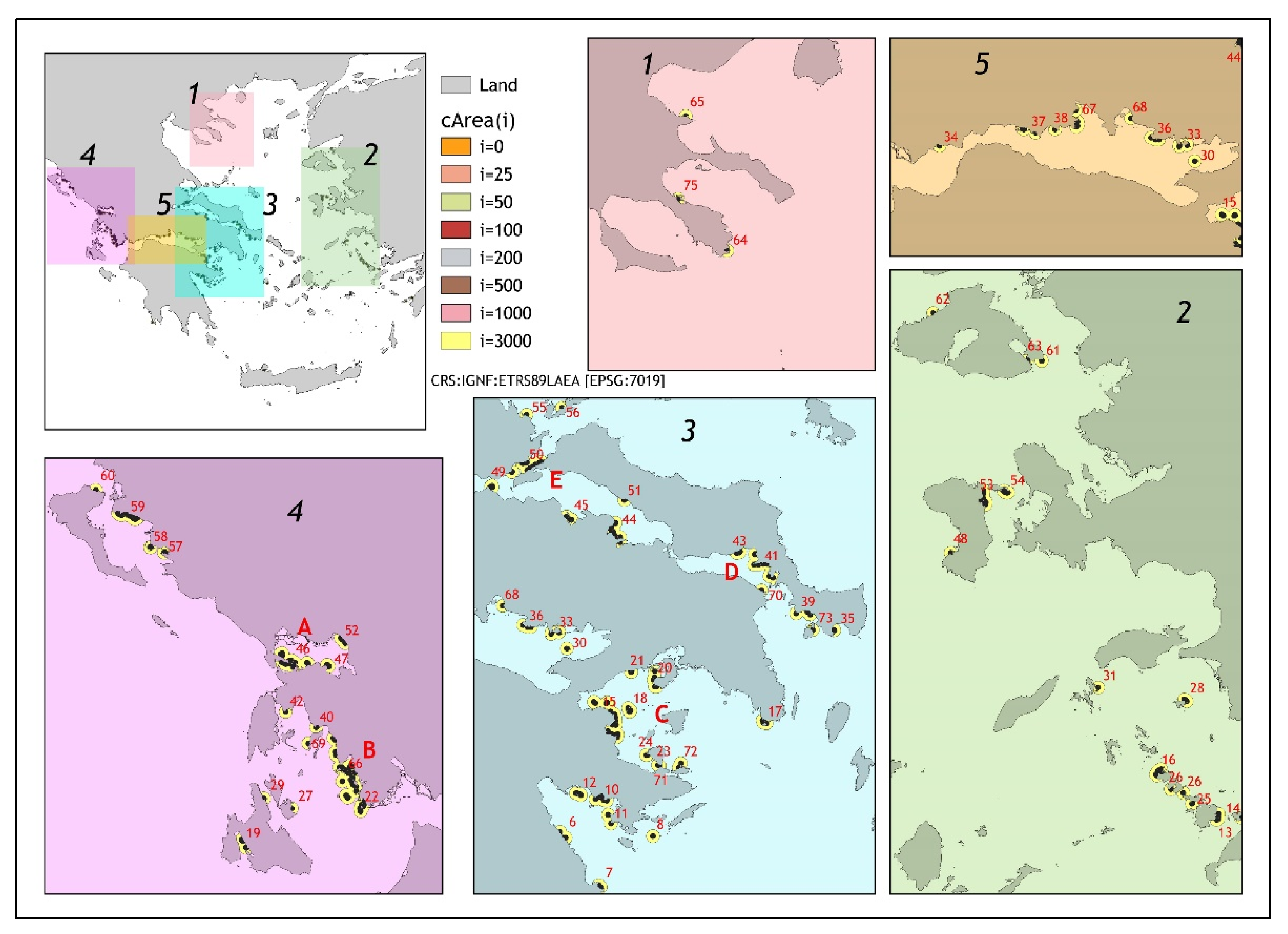
The buffer area (
cAreai*) created by one or more cage arrays for each category
i, ignoring the individually overlapping areas that originated from each cage array (i: 0, 25, 100, 200, 500, 1000, and 3000 m are the distances from
l’s edge) (
cAreai*: common area of
l’s for distance i), was designed. From the layer
cAreai*, the removed area that corresponded to land provided the
cAreai that corresponded to the sea area of each impact i. For each
l, the functional volume per
cAreai (Vsl,i) where the
l participated in its creation was calculated.
Vs is the farming volume per unit of the impacted area while it expresses the level of farming pressure on the impacted area, which can be used as a measure of the impact’s intensity. The shorter distance of the cage array from the shoreline (Dst) was estimated as the shorter distance of the
cArea0 layer from the land layer. The land layer was provided by the European Environment Agency [
48] (accuracy 50 m).
For each
l, a set of variables (MVs) was gathered:
Vl, AsNC
l,
cAreal,I, and
Vsl,i. To identify linear relationships among the MVs, factor analysis (FA) ((rows) X (columns); (
l) X (MVs)) was applied. The factor loadings per factor (
Fn) indicated the weight of each variable to the corresponding factor while the factor scores per factor (
Fscores) are the linear result of the initial variables with respect to this factor [
49]. Due the fact that the MVs showed a non-normal distribution (Shapiro–Wilk W test < 0.90;
p < 0.05), before the PCA application, the MVs were log-transformed (log-MVs) [
46].
The l values that create the common cArea3000 are members of the spatial cluster j (scj) of cage arrays while the maximum distance between l for membership is 6 km. For scj, the mean value (mFscores) and standard deviation (SDFscores) of the factor scores were estimated.
To examine the similarities of the Fscores between the sc, a clustering technique based on the Ward linkage and squared Euclidean distance ((rows) X (columns); (sc) X (mFscores, SDFscores of Fn)) was used.
Levene’s test was applied to test for significant differences between the variance of the variables:
l, Dst,
cArea3000,
mFscores, and
SDFscores among
sc groups. In cases where the variance was not statistically significant (Levene’s test;
p > 0.05), analysis of variance (ANOVA;
p = 0.05) to test for significant differences in these variables among
sc groups and Bonferroni test were applied to check which
sc groups differed from each other. In cases where the variance was statistically significant (Levene’s test;
p < 0.05), the Kruskal–Wallis test was used to check for significant differences between these variables among the
sc groups and the Mann–Whitney test was sued to check which
sc groups differed from each other [
46].
As the legislation (Common Ministerial Decision No 31722/2011, FEK 2505 ratified on 4 November 2011) and Areas Organized for Aquaculture Development (AOAD) are defined, more or less, on the concept of the Allocated Zone for Aquaculture (AZA) [
40,
50], the existing fish farming site units fall under AOAD. The AOAD is classified according to the priorities and the type of development into five categories: (A) particularly developed areas requiring improvement, modernization of farms and infrastructure, and better environmental management; (B) areas with significant scope for development; (C) remote areas with significant scope for development; (D) areas with particular environmental sensitivity requiring the adaptation of existing farms to the specific characteristics of the aquatic environment; and (E) suitable areas for further development of aquaculture (includes islands and shorelines with low farming activity).
Mapping on the coordination reference system ETRS89LAEA-ETRS89 Lambert Azimutal Equal Area was projected.
3. Results
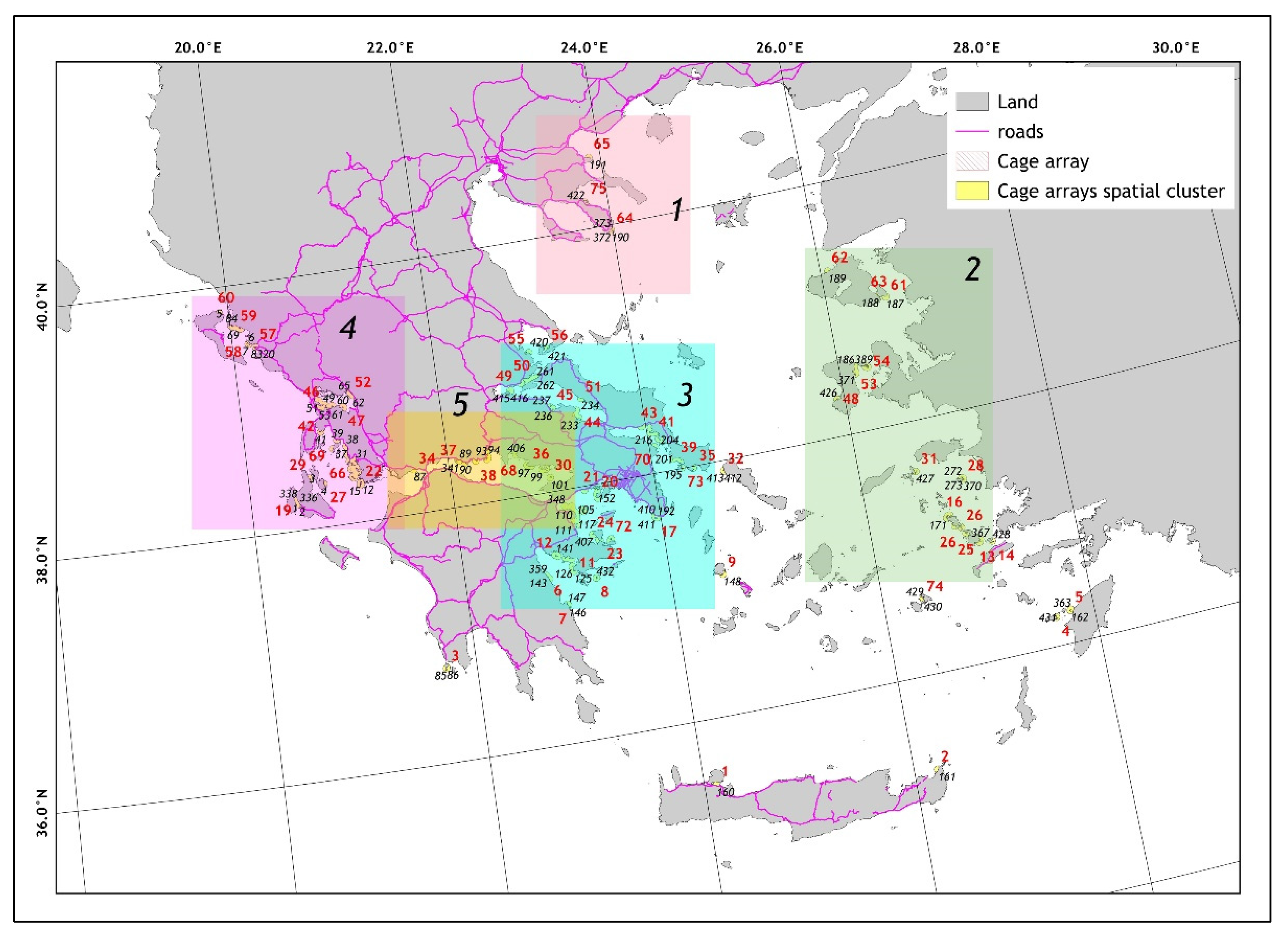
In total, 433 fish farm cage arrays were recorded along the Greek coastline during the period 2016–2017 (
Figure 1). The mean (±SD) farming volume of the arrays was 38.62 ± 26.88 × 10
3 m
3, the mean number of squared cages was 5.43 ± 10.22 cages, the mean number of circular cages was 16.44 ± 12.69 cages, and the mean shorter distance of the cage arrays from shoreline was 154.55 ± 177.23 m. The total farming volume of the arrays was 16,726.6 × 10
3 m
3 while the total number of cages was 9977 (2355 squared and 7122 circular cages) (
Table 2).
In total, 1926
cAreas were recorded. The number of
cAreas ranged from 75 to 433 (at
i = 3000 and 0, respectively) (
Figure 1). The mean
cArea (±SD) ranged from 0.015 ± 0.013 to 32.78 ± 29.52 km
2, the mean number of cage arrays (
l) ranged from 1.0 ± 0.00 to 5.77 ± 8.65 arrays and the total
cArea per
i ranged from 6.51 km
2 to 2469.15 km
2, at
i = 0 and 3000 m, respectively (
Table 3).
Factor analysis extracted five factors (F1, F2, F3, F4, and F5) explaining 83.69% of the initial variance (
Table 4). Using a cut-off value of ±0.50 for the factor loadings, F1 was positively associated with the
cArea0,
Vl, and
Vsi for
i > 0, describing the
sc’s intensity of impacts. The F2 was positively associated with
cArea500,
cArea1000, and
cArea3000 and negatively associated with
Vs500, Vs1000, and
Vs3000, describing the high-distance (>200 m) impacted areas and the intensity of impacts. F3 was positively associated with
cArea50, cArea100, and
cArea200, describing the mid-distance (50–200 m) impacted areas. F4 was positively associated with
cArea0 and ANCS and negatively associated with
Vs0, describing the local (under cages
i = 0 m) impacted area and its intensity of impact and type of cages. Finally, F5 was positively associated with
cArea25 and negatively associated with
Vs (
Vs25), describing the low-distance (
i = 25 m) impacted area and its intensity of impact.
The cluster analysis applied to
sc was composed of more than one cage array while this group made the
sc group 1. The cluster analysis of the
Fscores revealed another five groups of cage array spatial clusters (
sc group 2 …
sc group 6). The mean number of arrays differed among the
sc groups (Kruskal–Wallis;
p < 0.05). In
sc group 1, there were 27 spatial clusters; in
sc group 6, there were 15 spatial clusters; in
sc groups, there were
2 and
3 and 11 and 10 spatial clusters; and in
sc groups 4 and
5, there were 7 and 5 spatial clusters, respectively (
Table 5).
The
sc group 6 has a greater number of cage arrays (5–48), followed by the
sc groups 2, 3, 4, and
5 (2–11 cages arrays) while the
sc group 1 has the lowest number of cage arrays (1 cages array) (Mann–Whitney test:
p < 0.05). The mean
cArea3000 of
sc group 6 was greater at 68.31 (±49.50) km
2 than
sc group 2 and
sc group 3 (31.18 ± 8.37 and 36.37 ± 10.40 km
2, respectively) and also greater than
sc group 1, sc group 4, and
sc group 5 (17.86 ± 4.72, 22.84 ± 11.20, and 17.05 ± 2.56 km
2, respectively) (ANOVA on log-transformed data;
p < 0.05; Bonferroni test;
p < 0.05). The mean shorter distance of the cage arrays from the shoreline was higher in the
sc group 6 (178.59 ± 208.46 m). Most of the functional farming volume was covered by the
sc group 6 (63.37%) while the other
sc groups shared 3.43% (
sc group 5) to 12.45% (
sc group 2) of the total functional farming volume (
Table 5).
The ANOVA showed statistically significant differences regarding the mFscores between the sc groups (p < 0.05). The Bonferroni test indicated for F1 Fscores:
[sc group 4] < [sc group 6 = sc group 3 = sc group 5] < [sc group 5 = sc group 1 = sc group 2]
for F2 mFscores:
[sc group 1 = sc group 5] < [sc group 4 = sc group 2] < [sc group 2 = sc group 3] < [sc group 6]
for F3 mFscores:
[sc group 1 = sc group 2 = sc group 3 = sc group 4] < [sc group 5 = sc group 6]
for F4 mFscores:
[sc group 4] < [sc group 2 = group 6 = sc group 1 = group 5] < [sc group 1 = group 5 = sc group 3]
for F5 mFscores:
[
sc group 2] <
sc group 1 = sc group 2 = sc group 3 = sc group 4 = sc group 5 = sc group 6] < [
sc group 6] (Bonferroni test;
p < 0.05) (
Table 6).
The Kruskal–Wallis test showed statistically significant differences regarding the SDFscores between the sc groups (p < 0.05) only for F3 SDFscores and F4 SDFscores. The Mann–Whitney test indicated for F3 SDFscores that:
[sc group 4 = sc group 5] < [sc group 2 = sc group 3 = sc group 4 = sc group 5] < [ sc group 6]
and for F4 SDFscores:
[sc group 3] < [sc group 3 = sc group 5] < [ sc group 2 = sc group 5 = sc group 6] < [sc group 4]
It is noted that in the Kruskal–Wallis test, the
sc group 1 was excluded as the
SDFscores for all
Fs were 0 (
Table 6).
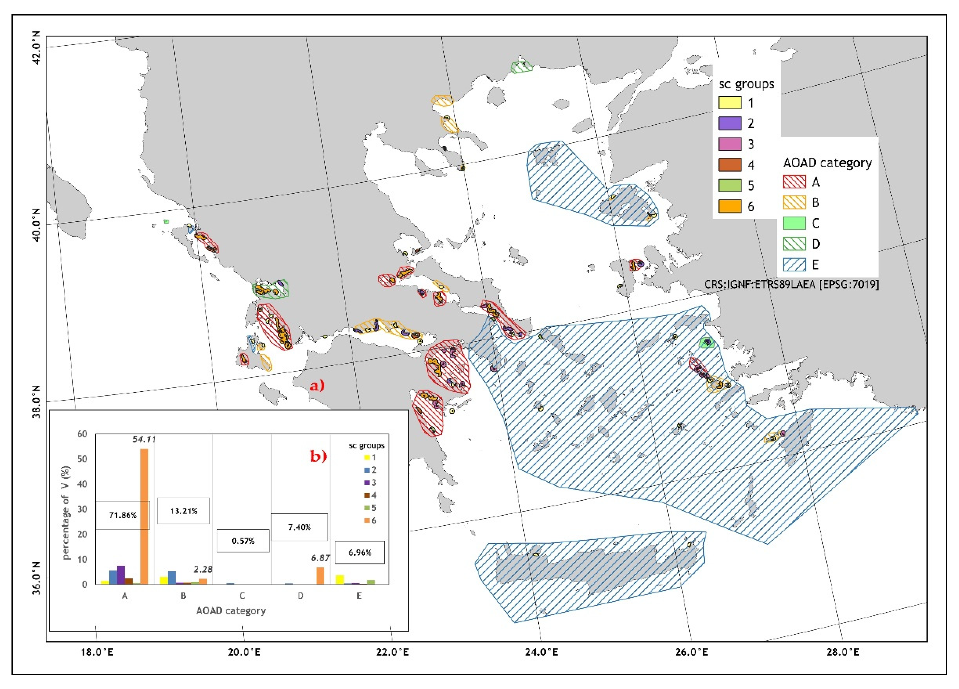
The 5 more extended
scs (belonging to
sc group 6) covered 35.5% of the total
V and located in west-central Greece (ID: 66; 204 km
2; 11.2% of total
V), Saronikos Gulf (ID:15;142 km
2; 7.9% of total
V), Amvrakikos Gulf (ID: 46; 109 km
2; 5.9% of total
V), South Evoikos Gulf (ID: 41; 85 km
2; 5.9% of total
V), and North Evoikos Gulf (ID: 50; 73 km
2; 5.9% of total
V) (
Figure 2).
The greatest farming volume was recorded for the AOAD category A (71.86% of the total volume) with the dominant contribution of
sc group 6 (54.11% of total volume) while the farming volume contribution of the other AOAD categories ranged from 0.57 to 13.21% of the total volume (
Figure 3).
4. Discussion
The seabass and seabream culture in Greece began in the early 1980s, and after 1995, it entered a stage of maturation. This stage, at a technological level, was best known for the trend of increased production volume by changing the size and shape of the cages being used (from squared and cyclical cages with s perimeter < 40 m to cyclical cages with a perimeter > 40 m) [
40,
51]. A study based on satellite images for the period 2001–2011, recorded a considerable change toward larger cages accompanied by the uninstalling and/or relocation by new installations of farms [
44]. In the present study, for the period 2016–2017, along the Greek shoreline, 9477 cages were recorded. This result is in line with a recent study [
37] for June 2016 while a previous study [
31] in 2006 recorded 10,422 cages. This difference is somewhat expected due to the inter-temporal modification of farm structures from small to larger cages [
41,
51] to increase the production volume. According to our findings, the independence of the cyclical cages’ number percentage of cage arrays (ANCS) by the functional farming volume (
Vl) (
Table 4: F1) indicates that the modification of farm structures is reaching the climax phase.
The farming activity is located near the shoreline, with most of it (81.9% of the total functional farming volume) being located along the mainland shoreline and in particular in the central part of country (
Figure 1), in close vicinity to the main road network. Farmed fish is an export-oriented product for major EU markets [
42], so the small distance from the national highways to the major ports Igoumenitsa and Patras is an asset to the supply chain.
The area that may have been environmentally impacted by fish farming activity ranged from 6.51 km
2 (under the cages arrays: impact on bentho-communities [
6,
7,
8,
9,
10,
11,
12]) to 2459.15 km
2 (zone 3000 m around the arrays: impact on nekton-communities demography) [
13,
14,
15,
16,
17,
18,
52,
53] (
Table 1). According to the higher common zone of cage arrays, 75 spatial clusters were created (
Figure 2). Inside the spatial cluster, the cage array members can be considered as a field of wild fish’s attraction and concentration [
13,
14,
16,
25,
28] since connectivity through wild fish is apparent [
17] through the escape of farmed fish to the wild and vice versa [
52]. Moreover, wild fish do not seem to participate in the transmission of diseases and parasites in the spatial cluster [
54] for escaped fish, which is a true fact [
53]. Thus, the spatial clusters should be considered as a delimited area for the research and management of diseases (namely, disease management area [
55]) and of escaped fishes.
Greek legislation (Common Ministerial Decision No 31722/2011, FEK 2505 ratified on 4 November 2011) provides detailed definitions regarding the fish farm unit (owning entity), the park, and the arrays of cages. The distance among the parks of a unit can be between 100 and 250 m and higher than 500 m among the units. Moreover, the allowed carrying capacity (related to the functional volume) of a specific location (in practice, the leased area) is controlled by several parameters, such as the currents’ velocity, geomorphology due to the openness/exposure of a location to open sea, bathymetry, and distance of thee farm from the shoreline, etc. (121570/1866/12 June 2009 common newsletter of Ministry Environmental, spatial planning and Ministry Rural development and foods of Greece) [
7].
Although the legal regime is recent, Greek marine finfish farms operate under the legal specifications [
7]. The above legal guidelines have led to a spatial pattern of cage arrays in which the short-distance zones (
i < 50) are impacted, absolutely, by one cage array while the mid-distance (50–500 m;
i: 50–500) and long-distance zones (>500 m;
i > 500) are impacted by cage arrays belonging to different parks of the same unit and by different units, respectively. This latter finding is based on a study of 230 farm units (equal to the number of
cArea200′s) comprising 1.88 ± 1.47 cage arrays (
Table 3), which is an estimation is close to the number of Greek finfish marine farms that was recorded in 2013 (240 farms) [
7].
The factor analysis revealed that the mean functional volume of the cage arrays of a spatial cluster controlled the intensity of impacts at the studied distances (at least for distances ≥ 25 m;
i ≥ 25) (
Table 4: F1). F2, F4, and F5 support an inversely proportional relationship between
cAreas500–3000, cAreas0, and
cAreas25 and their impact’s intensity, respectively, while
cAreas50–200 was not related to its impact’s intensity (F3). For the cases of
i = 0 and
i = 25, the inverse relationship between
cAreas and
Vs is expected as the cage’s establishment in a cage array occurs at a given distance among them, and so, by increasing
Vl of the array via the addition of cages, this increases
cArea. In the case of
i = 0, it seems that the usage of cyclical cages, for a given
Vl, increases
cArea0 due to their mooring technique, which requires a greater distance among them than for squared cages. Regarding
cArea500–3000, it is easy to estimate the integration of a cage array belonging to another farm unit (minimum distance between units ≥ 500 m), which increases
cArea500–3000 exponentially, resulting in an inverse relationship between
Vs and
cArea.
On the other hand, keeping in mind the shorter distance from the shoreline for most of the cage arrays is 50–200 m (
Table 2), the variation in the local shoreline geomorphology affects the size of
cAreas50–200 and a positive relation between the local shoreline geomorphology variation and the variance of
cAreas50–200 is expected, driving their independency by their own
Vs. Furthermore, the relatively low accuracy of the shoreline capturing the land layer (around to 10% at
i = 50 to 3% at
i = 200; estimated as the error zone that is 2 times the accuracy of the land layer by a width of 50 m multiplied by the 100 m length of shoreline;
Table 3) in relation to the size of
cAreas increase the variance of
cAreas. Finally, these zones refer to the cage arrays that comprise a unit. As per the abovementioned factors, the carrying capacity (related to the functional volume) of a specific location is controlled by several parameters [
7], which lead to an expected variation of
Vl for given
cAreas50–200.
The aquaculture industry operates on the condition that a particular regulatory framework is used, with provision of an Allowable Zone of Effects (AZE) as has been used by Scottish Environment Protection Agency (SEPA) in Scotland [
56], where specific environmental quality standards pertain. This is true considering that specific environmental quality standards in the zone up to 100 m from the cages’ edges in the direction of the common currents are allowed (121634/7242/20 December 2019 newsletter of Ministry Environmental and Energy). Thus,
cArea100, as estimated in the present study, could be considered as the AZE according to the allowed specific environmental quality standards as defined by Greek legislation. Additionally, numerous fish farms participate in ASC’s (Aquaculture Stewardship Council’s) aquaculture certification program for recognition and to gain the reward of responsible aquaculture. From its standards comes the definition of AZE, which is defined as a zone of 25 m when the AZE has not been defined using a robust and credible modeling system [
43].
The 15
sc values (out of 75
sc) that constitute the
sc group 6 cover 63.2% of the total functional farming volume (
Table 5), indicating that Greek marine fish farming activity shows a high level of spatial aggregation. On the other hand, the majority of fish farming activity showed a relative moderate intensity of impacts (
sc groups 3,
5, and
6; cover 75.9% of the total functional farming volume (
Table 5). After six years from the legislation application, the distribution of farming activity among the AOAD categories seemed to not have changed (as well as the production [
41]), which may be due the deceleration of the farming activity growth rate, thanks to the Greek debt crisis [
40].
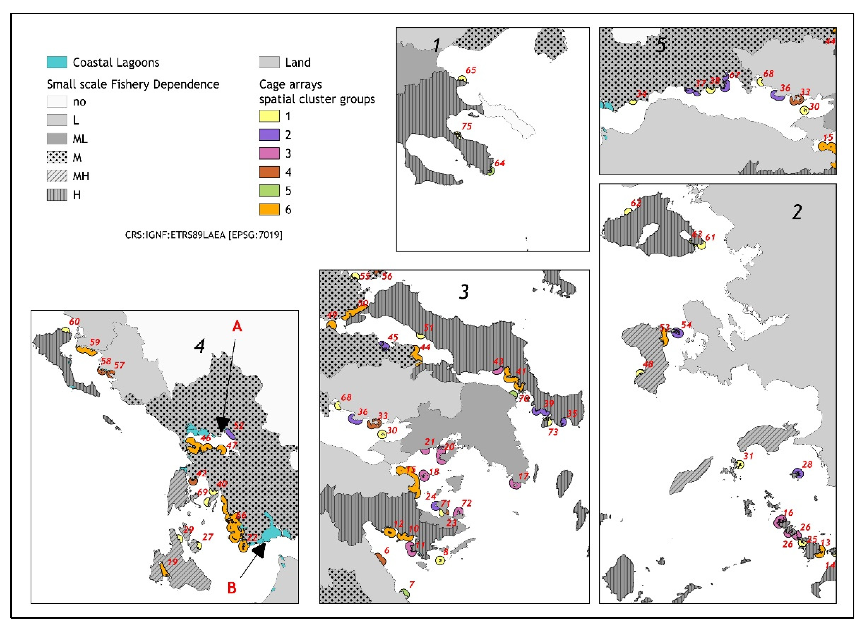
Locations with a high clustering of farms showed a notable increase in small-scale fishery production [
28]. The fact that these zones belong to the coastal zone of regions that show a relative dependence on small-scale fishery [
57] indicates a possible important conflict for sites in the vicinity of farms and synergy for sites out of farms’ vicinity, among the two activities (
Figure 4). On the other hand, the presence of extensive fish farming activity (
sc ID: 66, 22) in the vicinity of Mesolongi-Aitoliko lagoons (protected habitat: Natura 2000) and in Amvrakikos Gulf and in the vicinity of their lagoons (also protected area: Natura 2000) (
sc ID: 46, 47, and 52) has played a crucial role not only in lagoonal ichthyofauna biodiversity changes [
58] but also in the reduction of fishery production of the lagoon [
59,
60], affecting the functions of the lagoon habitats (
Figure 4).
A number of factors controlling the accuracy of the shape and size of the zones and the intensity of impacts are: (a) the hydrodynamic conditions of each location play a key role in the dispersion of waste [
6,
26,
61,
62,
63]; (b) in the present study, the impact zones were estimated as a projection on the sea surface so the actual impacted area (especially that on the substrate:
i = 0 up
i = 500 m) of the bottom is expected to be greater than was estimated due to the deformations of the bottom terrain, with small variations in the bathymetry resulting in significant changes in the sedimentation pattern [
64]; (c) the assumption that the intensity of impacts only depends on the functional volume while various patterns of feeding occur among farms [
65,
66]; (d) changes in the cage array locations (relocation, add or removal) can change the impact zones sizes; (e) the accuracy of the land layer affects the size estimation accuracy of the mid-distance impact zones. An improvement would be to estimate the shoreline using satellite images with a higher accuracy (i.e., Sentinel 2; spatial resolution of 10 m [
67]) or to perform manual correction following the coastline on the Google Earth images; and (f) the progressive decrease in the impact intensity according to the distance from the cage arrays (see the citations in
Table 1) was not considered. An improvement is to decrease the grid cell size and the cell’s weighting according to the distance.


