Abstract
Future nearshore wave energy converter (WEC) arrays will influence coastal wave and sediment dynamics, yet there are limited numerical methodologies to quantify their possible impacts. A novel coupled WEC-Wave numerical method was developed to quantify these possible influences on the nearshore coastal wave climate. The power performance of an Oscillating Surge Wave Energy Converter (OSWEC) array was simulated to quantify the wave energy dissipation due to the array. The OSWEC’s effect on the local wave climate was quantified by a novel coupling of two numerical models, WEC–Sim and XBeach. WEC–Sim characterizes the power extraction and wave energy transmission across the OSWEC, while XBeach captures the change in wave dynamics due to the WEC and propagates the waves to shore. This novel methodology provides the ability to directly quantify the impact of the effect of a WEC array on the local wave climate. Three case studies were analyzed to quantify the impact of a single WEC on breaking conditions and to quantify the impact of number of WECs and the array spacing on the local nearshore wave climate. Results indicate that when the WEC is placed 1100 m offshore, one WEC will cause a 1% reduction in wave height at the break point (). As the WEC is placed further offshore, the change in will become even smaller. Although the change in wave height from one WEC is small, WEC arrays magnify the cross–shore extent, area of influence and the magnitude of influence based on the spacing and number of WECs. For arrays with 10 or 15 WECs, the cross–shore extent was on average 200–300 m longer when the WECs were placed one to two WEC widths apart, compared with being spaced three or four widths apart. When the spacing was one WEC width apart (18 m), there was a 30% greater spatial impact on the nearshore region than arrays spaced three or four widths apart. The trend for the average transmission coefficient is within 5% for a 5, 10 or 15 WEC array, with a cumulative average of 78% transmission across all conditions.
1. Introduction
In 2021, the Intergovernmental Panel on Climate Change’s report showed that the current environmental crisis necessitates a dramatic shift away from fossil fuels towards sustainable and renewable energy solutions [1,2,3]. Marine renewable energy solutions, such as wave energy converters (WECs), have the potential to fill some of the energy requirement gaps ([4,5,6,7,8,9]). As the development of WEC arrays is considered, the impact WECs have on the nearshore wave environment must be characterized [10,11,12,13,14]. This study quantifies the impact of nearshore WECs and WEC arrays on the coastal wave environment. Through the development of a novel soft-coupled modeling technique for WEC-Wave interactions, this study documents how the sea-state dependent power production of a WEC array has widely varying impacts on the wave climate onshore of the array.
Göteman et al. [15] present the current state of the art of WEC array modeling and found that the layout will have an impact on the performance of the park.
Additionally, Liu et al. [16] found that the OSWEC’s power performance will be significantly influenced due to the WEC layout, and both Liu et al. [16], Noad and Porter [17] have suggested optimal layouts for the OSWEC.
Many papers have reviewed, through numerical modeling [18,19,20,21,22] or physical tests [20,23,24,25,26], the effects of a WEC on sediment transport. In particular, Millar et al. [19] discuss a WEC array’s performance and its effects on coastal erosion, which is defined as the movement of sediment, rocks, or land away from the shoreline due to the cumulative forces of waves, currents, tides, and storms. Millar et al. [19] model the WEC array in its environment with SWAN, an open-source wave propagation model [27]. The WEC array is represented as a porous layer with coefficients that describe reflected, absorbed and/or transmitted wave power through/by the WEC. The results show that a wave farm with very efficient WECs (70% transmission, 30% absorption) produced a 0.13 m decrease in significant wave height ( between 2.5–2.6 m) at the shoreline. For a less efficient wave farm (wider spacing) with 90% transmission and 10% absorption, the largest change in is 0.04 m [19]. Overall, Millar et al. [19] contributed a methodology for using a porous layer in SWAN to represent the WEC’s impact on wave conditions with generalized transmission coefficients. However, the method neglects intrinsic information about the devices. Since the devices are represented as a porous layer with an idealized reflection and transmission coefficient, the device size, location and array density, as well as customized transmission coefficients across various wave conditions, are neglected and assumed negligible. Furthermore, unrecoverable and significant WEC viscous power losses are not considered in the calculation of the transmission coefficient. Prior research shows that viscous power losses are important for providing a more accurate calculation of the power extracted from the wave field [28,29]. Since this seminal research, many scientists have used similar techniques to model different types of WECs and their effects on coastal erosion.
A WEC array’s impact on coastal erosion is further investigated by Abanades et al. [26,30,31]. Abanades et al. [26] study the Wave Cat WEC and the variability in wave climate when the WEC array is placed at increasing distances from the shore (2 km, 4 km, 6 km). WEC–Wave array dynamics were quantified using SWAN and imported into XBeach to model sediment transport. Results show that for every 2 km closer to the shore, the WEC array decreases erosion by 5%; however, the shoreward footprint of influence or impacted area described by Equation (10) is also reduced. Abanades et al. [31] use the same technique as [19] to study the influence of WEC arrays on coastal accretion and find that wave farms decrease erosion but also decrease beach accretion. In contrast, Mendoza et al. [20] show that WECs produce localized accretion. These differing results show that inconsistencies in modeling due to the lack of accurate transmission coefficients have a significant influence on predicted coastal impacts. As with prior works, the transmission coefficients are inaccurate when the size of the device, location of the specific devices and power losses due to viscous drag are omitted. In prior studies, assumptions of idealized transmission and reflection coefficients over a large area do not consider the altered WEC performance for different wave conditions; thus, the results ignore changes in power production for different significant wave heights and energy periods, which are notably important [32].
In 2016, Sandia National Labs (SNL) developed a new technique for modeling a WEC’s impact on their surroundings, called SNL-SWAN [33]. The SNL-Swan method was initially developed by Smith [34]. The method was then expanded upon by SNL [35,36]. The SNL-SWAN method allows the user to directly import the “WEC power performance data in the form of power matrices” into SWAN to observe the WEC’s effect on the waves [29,37,38]. Chang et al. [37] test various WEC arrays and show that an Oscillating Surge Wave Energy Converter (OSWEC) with a width of 26 m obtains the largest decrease in wave height behind the device (), while also producing the largest intercepted power. Their research also showed that the device had no effect on the peak wave periods [37]. Luczko et al. [29] improved the fidelity of the transmission coefficient calculation in SNL-SWAN to include viscous drag and found that the accuracy of the transmission coefficient was improved by . David et al. [32] showed that when the model accounts for more of the relevant physics of the wave–body interactions, the model predictions are more realistic downstream, showing that increased fidelity can develop more accurate predictions of wave–body interactions. Typically, once an SNL-SWAN solution has been generated, it is imported into XBeach to observe the effect the wave variation will have on sediment transport [26,37]. Although the SNL-SWAN method works well to analyze wave transmission and sediment transport, it requires at least three models to accurately analyze the data, which is computationally expensive.
The method developed and detailed in this study is akin to that of SNL-SWAN’s; however, the presented method soft couples WEC–Sim and XBeach directly, eliminating the need for SWAN, decreasing the overall computation time and increasing overall result fidelity. The method allows for precise transmission coefficients to be calibrated for each wave condition by combining power absorption and power losses in the transmission coefficient (neglected in SNL-SWAN). The presented method also implements an array of WECs in specific cross–shore locations, as opposed to other models which use a generalized transmission coefficient across an area. Further, XBeach can model the effect of a WEC on nearshore coastal hydrodynamic and sediment transport processes, such as changes in wave height, wave run-up extent and shoreline change, where SWAN can only model changes in deep and intermediate wave characteristics. XBeach models have been validated for coastlines around the world and can provide illuminating insights into coastal change [39].
The major contributions for this paper are threefold: first, the implementation of viscous effects within the power losses calculation (due to the presence of the WEC); second, the development of wave height–wave period specific transmission and friction coefficients; and third, the coupling of a WEC model (WEC–Sim) with a nearshore wave model (X-Beach) rather than SWAN—the focus of most prior efforts.
Section 2 details the novel coupling method between WEC–Sim and XBeach. Section 3 presents the results of the coupling focused on case studies showing the influence of WEC arrays on significant wave height reduction region of influence onshore of the WEC. The case studies presented vary the WEC array’s cross–shore position, the spreading between individual WECs in an array and the number of WECs in an array. In Section 4 and Section 5, the results of the study are placed in the context of other work, and future work is suggested.
2. Methods
In this study, WEC–Sim is soft-coupled with XBeach to model a WEC array’s impact on nearshore hydrodynamics (the overarching modelling framework is shown in Section 2.6). WEC–Sim is a numerical model that simulates the wave-body interactions of a WEC [40]. In WEC–Sim, the device dimensions, hydrodynamics, mooring systems, and power take off systems are characterized and simulated for a variety of wave conditions. Power output, viscous losses, and body motions are outputted. XBeach is a numerical model that was initially designed to simulate hydrodynamic and morphodynamic processes and impacts on sandy coasts during a storm, however it has been extended to a wide range of applications [39]. WEC–Sim quantifies energy absorption and viscous losses from an OSWEC under a variety of wave conditions. Results from the WEC–Sim simulation are utilized in XBeach through a short-wave friction coefficient to simulate the WEC’s effect on the flow field and onshore wave climate changes. XBeach and WEC–Sim are both open-source models, allowing for increased access and continued improvement for and by researchers.
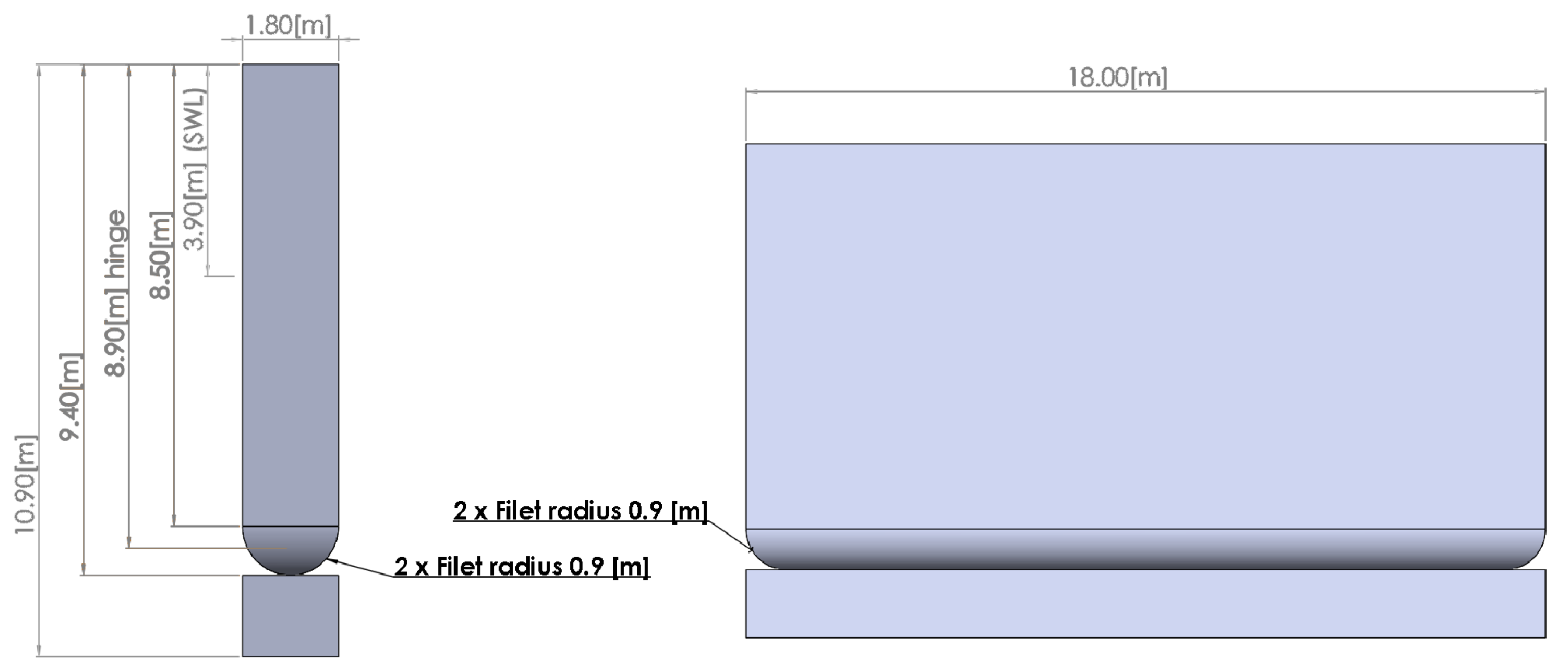
The coupling process and modifications to the WEC–Sim and XBeach models are discussed in the following subsections. For this study, an OSWEC is utilized. An OSWEC is a bottom fixed flap wave energy converter that rotates in pitch. The device is 18 m wide, 10.9 m tall and 1.8 m thick, as shown in Figure 1, and is typically oriented towards incoming waves. In XBeach, an idealized beach profile with a 1/100 dissipative slope and maximum depth of 10.9 m at 1090 m from shore is used as shown in Section 2.5.
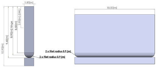
Figure 1.
WEC–Sim’s depiction of the OSWEC [40]. The device is a flap style WEC operating in pitch, with the bottom rectangle representing the base and the top, larger rectangle representing the flap.
2.1. Modeling the OSWEC in WEC–Sim
Linear wave theory and an irregular wave spectrum are used in WEC–Sim to calculate wave forces on the WEC. The Pierson–Moskowitz (PM) spectrum was used and is an appropriate choice for wave conditions on the west coast of the North America as shown in [41]. WEC–Sim uses the Cummins equation to model the wave-body interactions of the WEC [40].
where is the WEC rigid body acceleration and m is the WEC mass [40]. The excitation force (), and radiation damping force () are developed using a boundary elements method (BEM) solver, such as WAMIT (coefficients provided by the WEC–Sim Tutorials [40]). BEM solvers typically solve the Laplace equations for the velocity potential, which assumes the flow is inviscid, incompressible and irrotational [40]. The drag force () is included using drag coefficients () across a characteristic area (), which is chosen from empirical coefficients [42]. The fluid memory effect is captured by the convolution integral formulation in the Cummins equation. The PTO damping () is based on a sea-state dependent velocity proportional damping and is optimized for each wave period using WEC–Sim.
2.2. Optimizing the Model (Power Take off and Drag Coefficients)
Two adaptations are made to the OSWEC in WEC–Sim to improve the power performance of the device and increase the accuracy of the model. The first change to the baseline model was the inclusion of viscous drag coefficients () in Equation (1), based on significant wave height () and peak period (). The viscous drag coefficients used came from typical shapes defined in Avallone et al. [42]. The characteristic area () is included to scale the drag coefficients appropriately to the shape of the device in each degree of freedom. Secondly, the proportional PTO damping coefficient is optimized for each wave period to achieve the greatest power output. The values are shown in Table 1. The device’s intercepted power can be calculated using Equation (2), where is the relative body velocity.

Table 1.
Damping and drag forces used in this study for one example wave condition. The damping coefficients [] are calculated based on typical shapes, and the damping coefficients [] are optimized for optimal power performance for each wave period. The spring constant is represented by . Rx, Ry and Rz refer to the rotation in x, y and z directions, also known as roll, pitch and yaw.
The PTO damping coefficient () is optimized by testing a range of coefficients for each wave condition. For each damping coefficient, the average extracted power () is calculated across the entire wave simulation. The damping coefficient which provides the most power for that wave period is then used throughout the study. As damping increases in Equation (2), the power extracted by the device () also increases. The power continues to increase until the damping begins to reduce the body velocity. Consequently, the total extracted power will begin to decrease, as shown in Equation (2) [40]:
With the damping optimized and the drag coefficients calculated, WEC–Sim will provide realistic estimates for the extractable power from waves.
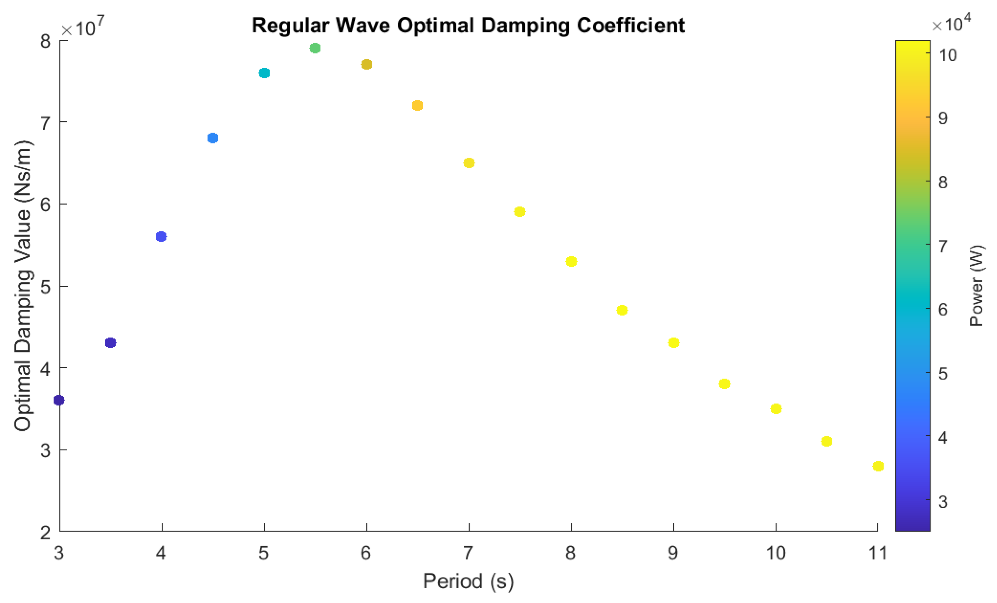
For each peak spectral wave period (), there is an optimal damping coefficient that allows the WEC to extract the maximum power. For each wave simulation in WEC–Sim, many damping coefficients were tested to determine which one produced the most power averaged across a 3000 s wave simulation.
Figure 2 presents a comprehensive image detailing the optimum damping coefficient for each wave period. A range of wave peak spectral periods were tested (3 s to 11 s) to observe how the intercepted power changes due to wave condition with the optimal damping coefficient. For the optimization process, the significant wave height was set to 2.5 m, since the damping coefficient is period dependent. The optimal power is period dependent as shown in equation 2, since the body velocity () responds to changes in wave period.
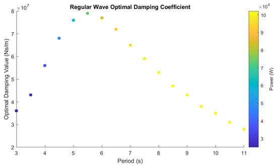
Figure 2.
Optimized damping coefficient for each Peak spectral wave period.
The image shows that as the wave period increases, the intercepted power also increases, until it reaches the maximum available power after 6.5 s. Additionally, the optimal damping coefficient increases until a peak wave period of 5.5 s, at which point it begins to decrease due to the wave–body interactions analyzed by WEC–Sim.
2.3. Calculating Power Extraction in WEC–Sim
For an irregular wave propagating toward the WEC, the incoming wave power can be calculated following [29], by
Once the incoming wave power or wave energy flux, () is known, WEC–Sim can generate the power extracted by the device (Equation (2)) and the power losses due to viscous drag (Equation (4)). In Equation (4), refers to each degree of freedom (heave, surge, sway, etc.). For each degree of freedom (N), the viscous force is multiplied by the velocity and summed across the other degrees of freedom. The equation is calculated for each time step (t) of the simulation, and the average is found across the entire time domain. For the OSWEC example, the pitch degree of freedom is of highest importance.
As introduced by Luczko et al. [29], the intercepted power () is characterized by summing the average power extracted by the WEC () and the average power losses () for each wave condition by
The transmission of waves past the device can be calculated using the three power terms following Luczko et al. [29] with
The transmission coefficient () is the percentage of power from the initial wave that is transmitted past the device. is most easily described as the ratio between the incoming wave height and the wave height in the lee of the device following Dean and Dalrymple [43], with
In this study, is obtained for a variety of wave conditions experienced on the Oregon Coast.
2.4. XBeach Background and Modeling Specifications
XBeach is an open-source software that models nearshore hydrodynamics and sediment transport. The model is typically used to study a storm’s effect on a sandy coastline over the course of hours to days [39]; however, many adaptations have been developed to increase the versatility of the software.
In XBeach, there are three methods of modeling wave energy dissipation: first, by using a wave friction coefficient; second, by using vegetation; and third, by modeling wave breaking. The vegetation technique allows the user to import specific characteristics (size, porosity, density) of vegetation at specific locations to dissipate waves, while the wave breaking technique is calculated when waves break in the nearshore region. In comparison, the wave friction coefficient adapts the energy balance equations and is applied throughout the water column [39]. It also provides one variable that is easily adapted to achieve the desired shadow effects in the wake region. The short-wave friction coefficient is used to mimic the behavior of the WEC in XBeach. The key factors that are needed to run an XBeach simulation include bathymetry, wave conditions, a wave modeling technique and the time span of the model.
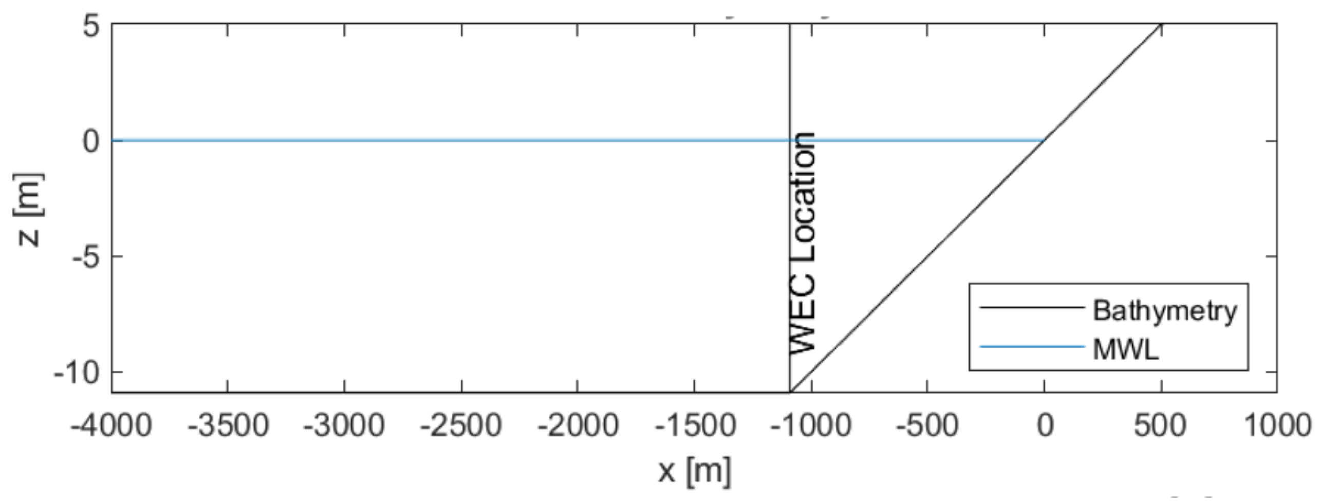
2.5. Bathymetry
In this study, a generic bathymetry is used. The bathymetry begins in 10.9 m water depth 4 km offshore. At 1100 m, the beach slope changes to 1/100, making the beach profile dissipative. The bathymetry and WEC location are shown in Figure 3.
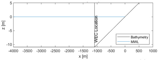
Figure 3.
Cross–section of the 3D bathymetry used in XBeach for all trials.
Additionally, to understand the influence of beach slope on wave transmission coefficients and the shoreward extent of the array’s influence on its wake, an additional 1/7 slope was tested for a limited set of wave conditions.
2.6. Wave Conditions and Modeling Techniques
XBeach provides various strategies for modeling wave dynamics. In this study, the wave boundary conditions were set using the PM spectrum in XBeach and WEC–Sim to model irregular waves [41]. Then, the waves propagate to shore using the Surfbeat version of XBeach. Surfbeat “resolves the short-wave variations on the wave group scale and resolves the long waves associated with them” [39]. To ensure that directional spreading was accurately modeled, the multi-directional method was used to solve “the time-varying wave action balance in XBeach” [39]. The multi-directional calculation controls the propagation of wave action in x, y and simultaneously by solving the 3D advection equation:
where A is the wave action and are the propagation speeds in each direction. is the dissipation due to wave breaking, is the bottom friction dissipation, and is the vegetation dissipation. is the intrinsic wave frequency and calculated using . The equation ensures that diffraction is accounted for and that the angle of wave propagation is recalculated throughout the simulation.
2.7. Modeling the WEC with the Short-Wave Friction Coefficient
To accurately model the WEC in XBeach, the short-wave friction coefficient is used (). The friction coefficient is incorporated into the short-wave dissipation coefficient () in the XBeach model, where
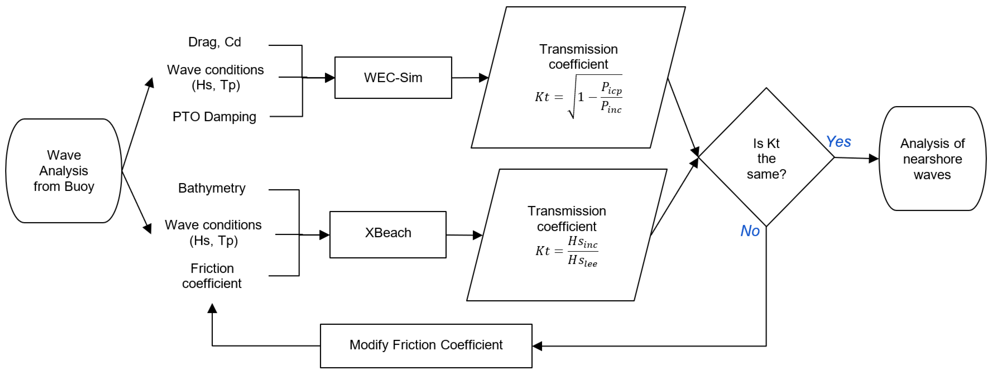
and is the water density, is the root mean squared wave height, is the first spectral wave frequency, k is the wave number, and h is the water depth. The friction coefficient was tuned to replicate the WEC–Sim results showing the effects of the WEC on wave dissipation. For each wave condition, the friction coefficient in XBeach was tuned to match the transmission coefficient () that was developed in WEC–Sim (Figure 4). Note, only affects the wave action equation and is unrelated to bed friction in the flow equation [39].
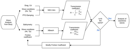
Figure 4.
Flow chart depicting the method for soft-coupling WEC–Sim and XBeach. The WEC–Sim trial is run first, and the WEC’s transmission coefficient (Equation (6)) is calculated. Then, the XBeach simulation is run using a randomly chosen friction coefficient. Once the simulation is completed, the average transmission coefficient is calculated (Equation (7)) in XBeach and compared with the from WEC–Sim. If the is the same, the friction coefficient is maintained. If it is not, the XBeach simulation is run again with a new until it matches the WEC–Sim .
To correctly model the wake effects in XBeach, the directional resolution was set to 5° to achieve accurate resolution. The wave spreading was set to 10 for the PM spectrum. The simulations were run for 2000 s to ensure that the waves had time to reach the beach.
2.8. WEC–Sim and XBeach Coupling Procedure
The process and methodology for coupling WEC–Sim and XBeach is depicted in Figure 4. The data from both XBeach and WEC–Sim are interfaced using Matlab. Simulations in XBeach are run using the command window. First, the WEC–Sim parameters (WEC dimensions, wave conditions, PTO damping and drag coefficients) are selected and the simulation is run to obtain the transmission coefficient of one WEC for each wave condition. The in WEC–Sim is calculated from Equation (6). Then, all wave simulations are run in XBeach, and the in XBeach is calculated from Equation (7) (see Section 2.3). Once calculated, the transmission coefficients from XBeach and WEC–Sim are compared. If the transmission coefficient is different, the friction coefficient in XBeach is tuned by trial and error, and the XBeach simulation is re-run until the transmission coefficients () match.
3. Results
In the following sections, the results detail the OSWEC performance, the correlation between the transmission coefficient in WEC–Sim and the friction coefficient in XBeach in Section 3.1. In Section 3.2, the general transmission of waves from the friction coefficient is explored. The three case studies presented in Section 3.3 and Section 3.4 show how the WEC array can affect the nearshore wave field and how the impact can change due to the array’s size, spacing and distance to the shore.
3.1. WEC–Sim () and XBeach () Transmission Results
The following results are based on wave resource assessments for Newport, Oregon [44]. For every wave condition, the incoming wave power, OSWEC power absorption and OSWEC power losses were calculated using WEC–Sim and are shown in Figure 5 and Figure 6 [45,46]. The simulations in WEC–Sim were run for 3000 s to ensure that the intercepted power matrices converged.
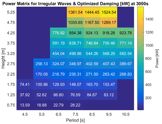
Figure 5.
The intercepted power () matrix for each wave condition calculated by WEC–Sim. The largest power generation can be found for the largest wave conditions.

Figure 6.
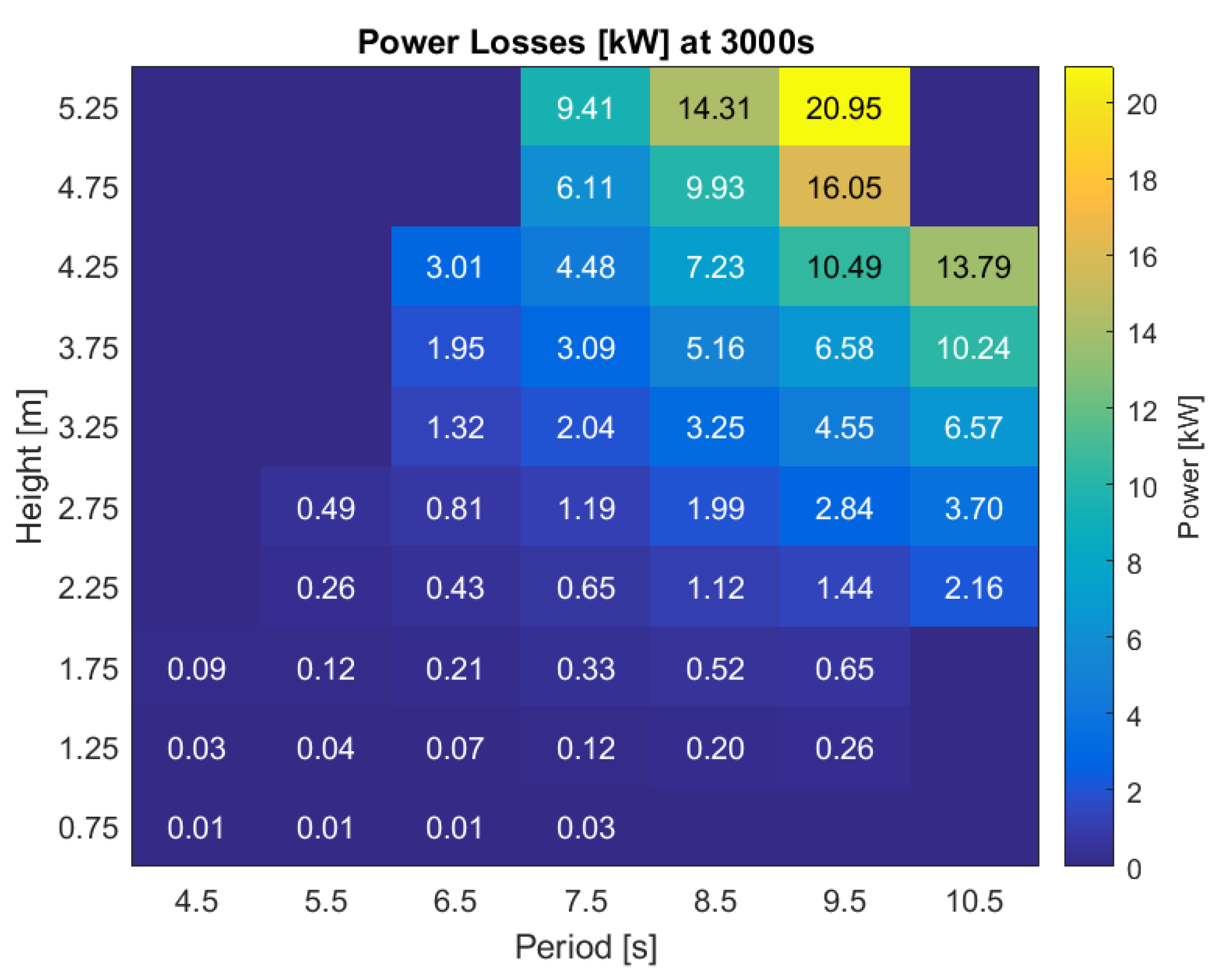
The power losses () matrix calculated in WEC–Sim across all periods.
For both the PTO power and viscous loss matrices, the highest power is extracted for the largest wave conditions. The PTO power is roughly two orders of magnitude larger than the viscous power loss.
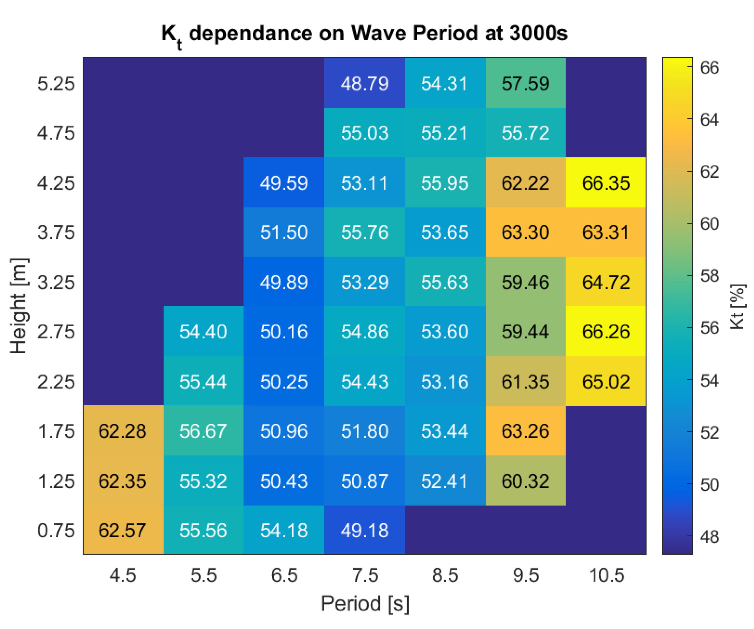
The transmission coefficients were calculated for various wave conditions using Equation (6). The results show that the OSWEC will absorb the largest proportion of the gross wave power at a wave period of 6.5 s. Furthermore, the largest transmission of waves or the smallest absorption of power occurs at the edges of the wave histogram (wave periods of 4.5 s and 10.5 s). The WEC–Sim transmission coefficients shown in Figure 7 are predominantly period-dependent, and changes by approximately with significant wave height (within each wave period). The WEC motion is excited by the frequency of the waves, which causes the device to be period-dependent.
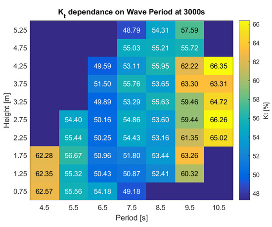
Figure 7.
The transmission coefficient () matrix for each wave condition calculated by WEC–Sim. The WEC absorbs the most power at a period of 6.5 s. The values are period-dependent and were averaged along each period to simplify the model.
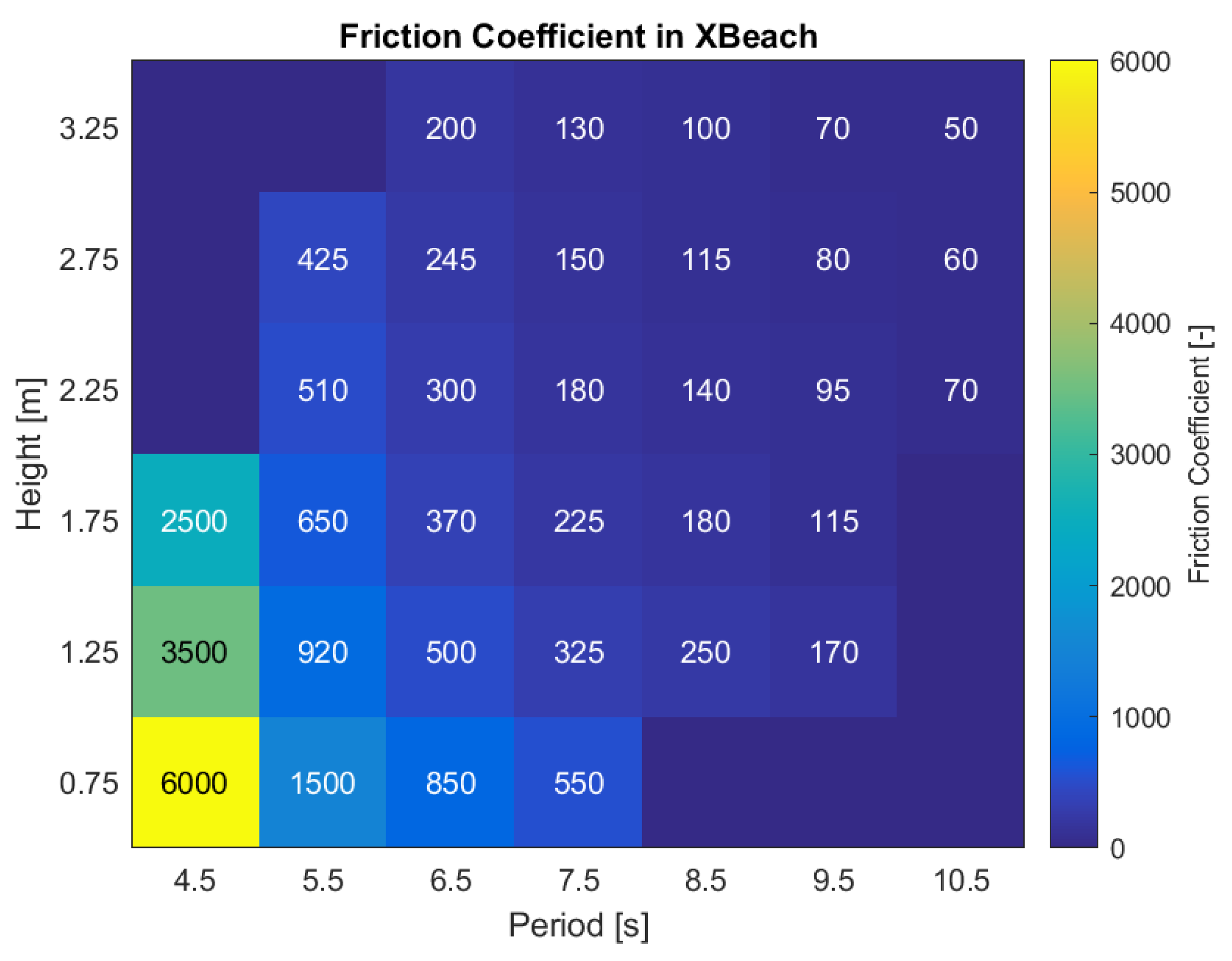
As explained in Section 2 and detailed in Figure 4, the WEC–Sim transmission coefficients were then used to create matching XBeach friction coefficients. As shown in Figure 8, the smallest significant wave heights and lowest wave periods necessitate the largest friction coefficient to replicate the WEC’s power absorption and the WEC–Sim transmission coefficient. In general, as the wave period and height increase, the friction coefficient decreases in a non-linear trend. This wide variation in XBeach friction coefficients is important to note since much of the prior published literature utilizes one static transmission and absorption coefficient across all wave conditions.

Figure 8.
The friction coefficients () calculated in XBeach corresponding to the period-averaged from WEC–Sim. The friction coefficient is selected due to the presence of one WEC in XBeach.
3.2. XBeach Nearshore Wave Transmission Results and Analysis
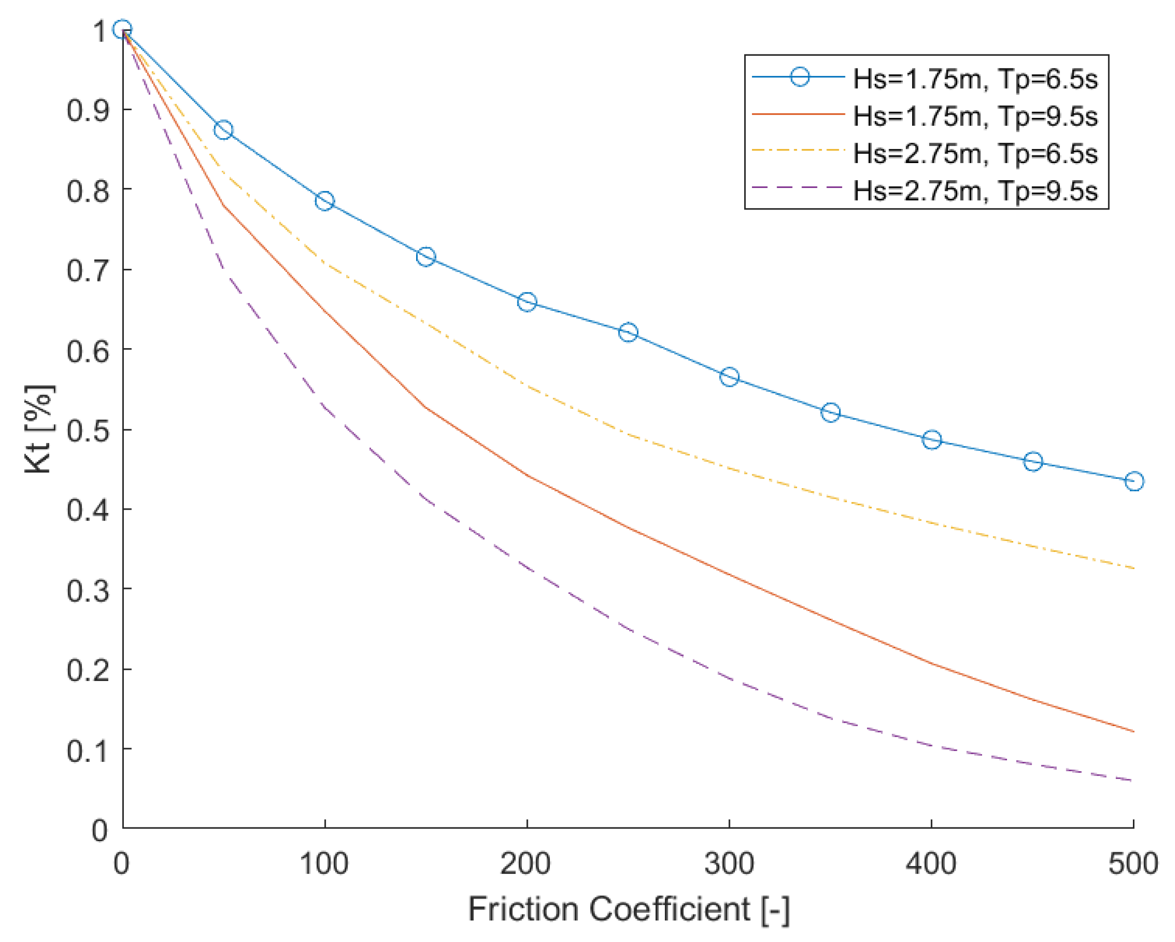
While the XBeach short-wave friction coefficient is reviewed in Lowe et al. [47], where it is used to calibrate the coastal impact onshore of a reef, there are few additional sources that document the short-wave friction coefficient behavior. To understand the behavior of the friction coefficient in XBeach, the general trend for has been plotted in Figure 9 for four wave conditions varying in wave height and wave period. The friction coefficients follow an exponential decay trend. The smallest wave condition [ m, s] continuously requires the largest friction coefficient to obtain appropriate transmission coefficient values. Increasing both wave height and/or period reduces the required friction coefficient. This non-linear trend in decreases as the value is reduced. It also appears that wave period has a larger impact on the friction coefficient trend than wave height—this is plausibly due to the greater impact of wave period on wave steepness.
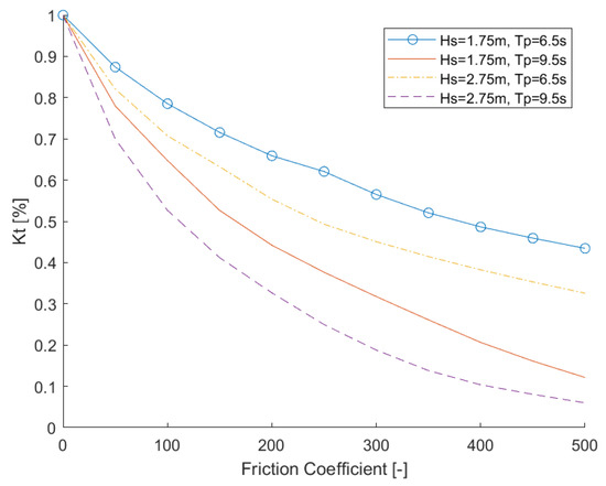
Figure 9.
Friction coefficient effect on the transmission coefficient across different wave conditions. Four wave conditions and various friction coefficients were tested. The corresponding transmission coefficient was obtained at the location of the WEC for each .
Figure 9 yields an easy way to determine the XBeach friction coefficient. Once a wave condition and corresponding WEC–Sim transmission coefficient have been calculated, the chart can be used to interpolate and obtain the XBeach friction coefficient. The friction coefficient may need to be tuned for each bathymetry to ensure that it produces accurate results.
Three case studies are explored to better understand the coastal impact from WECs and WEC arrays. The first case study analyzes the distance that a WEC should be placed from the shore to reduce the noticeable change in the nearshore wave climate. The second case study analyzes differing array sizes and layouts and their associated impact on nearshore wave climates. The first two case studies are performed on a 1/100 beach slope; for the third case study, the beach slope is changed to a much steeper 1/7 slope to explore the influence of beach slope on a limited set of wave conditions.
3.3. Case Study 1: WEC Location and Breaking Wave Height
Five WEC locations were individually tested to observe the effect on the wave height onshore of the device and at breaking. The WECs were placed 3000 m, 2500 m, 2000 m, 1500 m and 1100 m from the beach. Four wave conditions (significant wave height: 1.25 m, 2.25 m, and peak period: 5.5 s, 8.5 s) were tested.
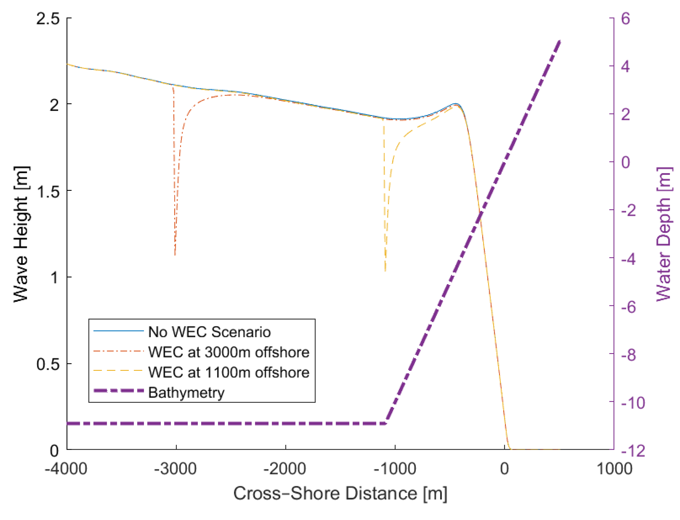
Figure 10 shows that when a single OSWEC is placed more than 1100 m offshore, it will have a negligible effect in the nearshore region. When the WEC is placed as close to the shore as possible (1100 m—based on bathymetry and OSWEC operating depth), the WEC will slightly decrease the wave height at the break point. For example, the WEC placed at 1100 m from shore showed a 0.024 m change in wave height for the wave condition with a wave height of 2.25 m and a period of 8.5 s. If one of the objectives of the WEC array is to create a change in wave height and associated reduction in erosional activity, the WEC array should be placed as close to shore as possible, given bathymetric constraints. For this specific bathymetry, the WEC will be placed at 1100 m for all further trials. The distance to shore in this case is limited by the height of the device (10.9 m) and the water depth, which is 10.9 m at 1100 m from the shore, as shown in Figure 3.
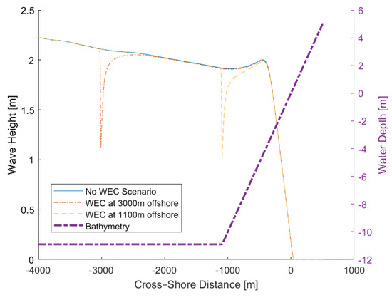
Figure 10.
Cross–sectional view of the 3D XBeach wave simulation in line with the WEC, showing a comparison of the placement of two WECs for a wave height of 2.25 m and a period of 8.5 s. The waves in the lee of the −3000 m WEC present a nearly negligible effect on the wave after 1100 m of propagation, while the WEC placed closer to shore shows a small decrease in the wave height at the break point.
3.4. Case Study 2: WEC Array Layout and Nearshore Wave Conditions
Although it is helpful to understand the impact that one OSWEC will have on its environment, it is rare that one OSWEC would be deployed for energy production or shoreline protection. Instead, it is expected that an array of OSWECs would be deployed. In this study, the optimal number of OSWECs and OSWEC spacing in the alongshore direction is investigated to quantify the impact on the waves and wake region in the nearshore environment.
Note that to quantify the impact of this WEC on its surroundings, all WEC array cases are normalized by the baseline case (without a WEC) to observe the absolute influence of the WEC array on wave transmission in the lee of the array. If the transmission value is large, it means that most of the wave height is transmitted past the device. As the transmission value decreases, more power is absorbed by the device, and the wave height in the lee of the device is smaller than the baseline wave height.
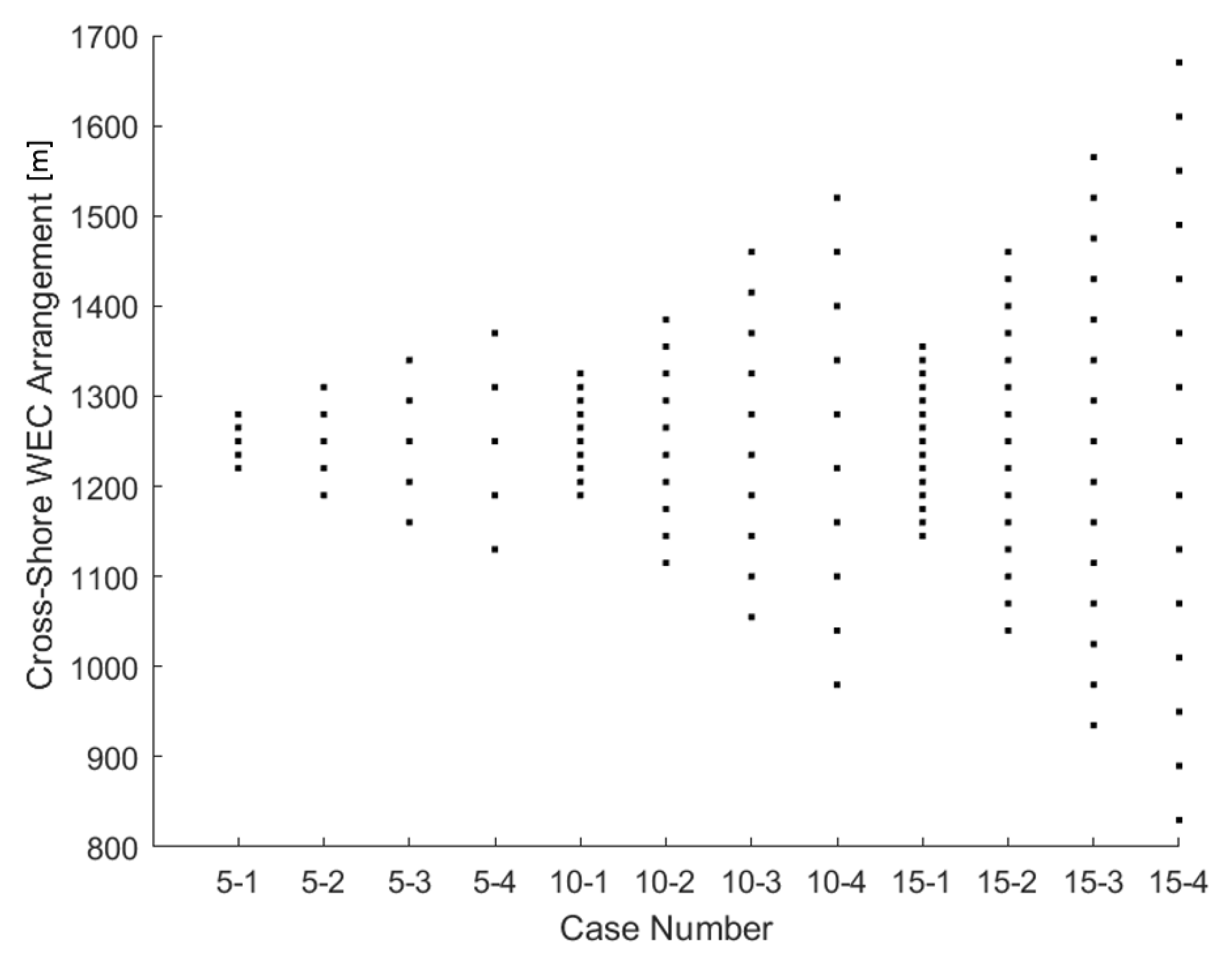
Three different WEC array sizes (5, 10, and 15 WECs) and four different WEC array spacings were presented to quantify the changes in the transmission coefficient across the domain. The WECs were spaced one, two, three or four WEC widths (D = 18 m) apart, as shown in Figure 11. Finally, three different wave conditions were tested; the wave height was set to 2.25 m, and the wave periods varied between 6.5 s, 8.5 s and 10.5 s. The wave conditions were chosen, since the wave height (2.25 m) spanned all three periods as shown in Figure 7 and provides a variety of wave conditions to compare. The WECs were all placed 1100 m away from shore. Each WEC spacing and array size combination was tested for all wave conditions, culminating in 36 case study simulations.

Figure 11.
The spatial arrangement of the WEC arrays for each case study. The x-label describes the number of WECs, and the number of widths spacing between each WEC. Each spacing is 18 m long; therefore, five WECs spaced at 18 m (1 WEC width spacing) are labeled “5–1”.
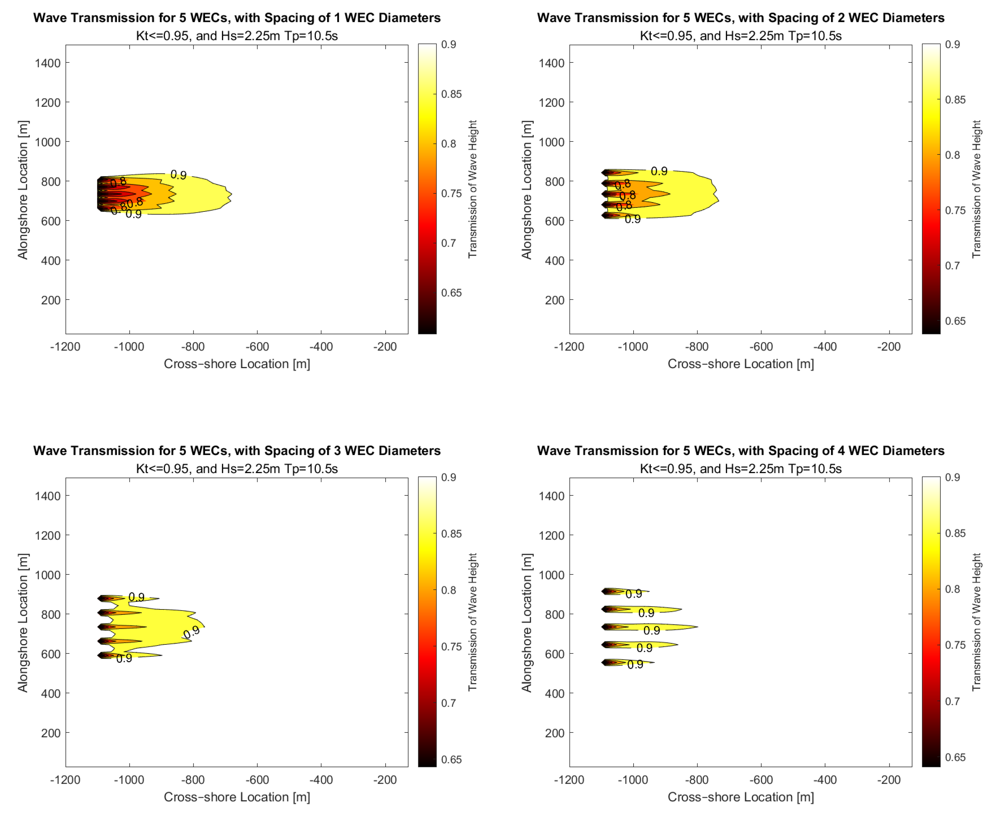
For each configuration, the transmission of waves past the WEC array was analyzed by dividing the specific WEC array case of interest by the baseline (no-WEC) case. In the following figures, the waves that were affected by the WEC array are shown. Figure 12, Figure 13 and Figure 14 show the transmission of waves in the lee of 5, 10 and 15 WECs with four different width spacings and one wave condition.

Figure 12.
Normalized wave transmission magnitude and extent of wave transmission influence in the lee of the 5 WEC array. The color bar shows the percentage of transmission in the wake region.
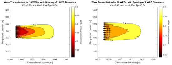
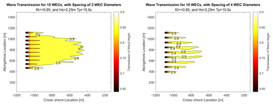
Figure 13.
Normalized wave transmission magnitude and extent of wave transmission influence in the lee of the 10 WEC array. The color bar shows the percentage of transmission in the wake region.
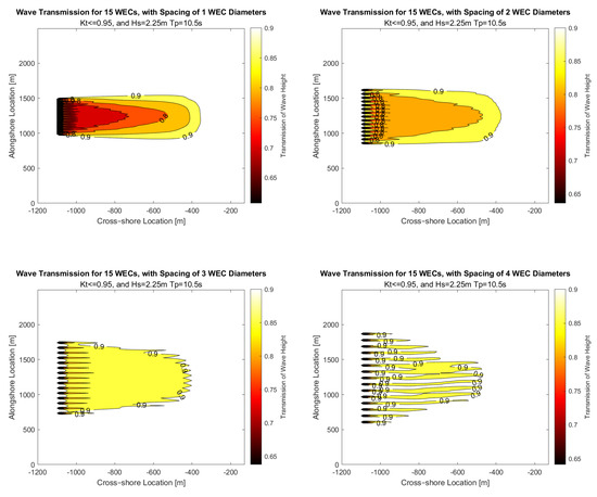
Figure 14.
Normalized wave transmission magnitude and extent of wave transmission influence in the lee of the 15 WEC array. The color bar shows the percentage of transmission in the wake region.
Note that when plotting the wake effects (Figure 12, Figure 13 and Figure 14), any transmission values greater than 95% were removed to ease the visual identification of change. For proceeding analyses of the results, only transmission values lower than 85% were used to focus on areas of significant change in the simulation results. Figure 15 and Table 2 show at the 85% level.
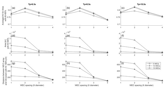
Figure 15.
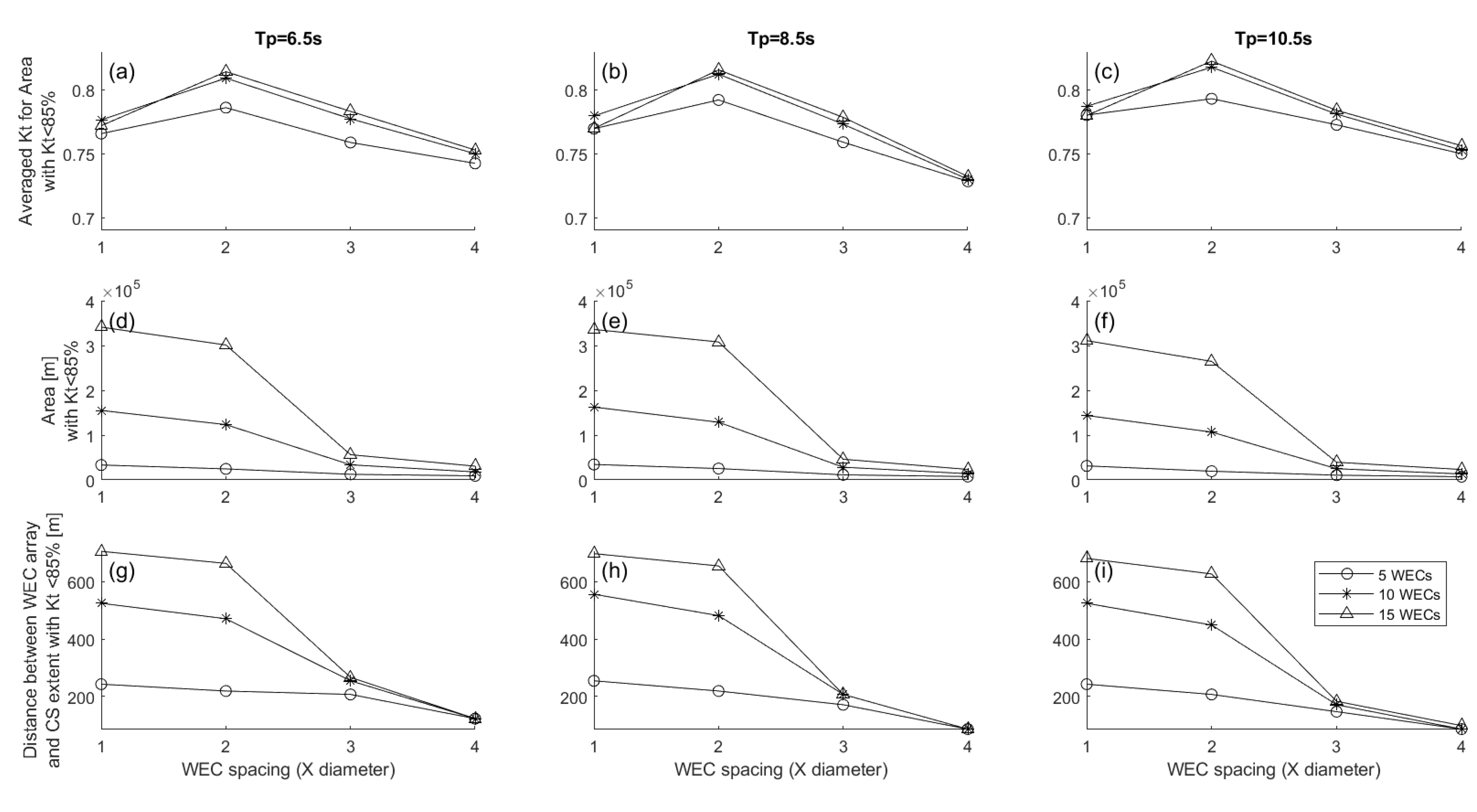
The average transmission coefficient across the region of wake influence (a–c). The area that is affected in the wake region (d–f). Panels (a,d,g), (b,e,h), and (c,f,i) are differentiated by wave period (6.5 s, 8.5 s, 10.5 s). In each panel, the x-axis shows the width spacing between each WEC, while the lines/markers refer to the size of the WEC array. Panels (g,h,i) show the cross–shore (CS) distance of wake influence from the WEC array to the onshore greatest extent of the wake region for different wave periods, WEC spacings and WEC array sizes. = 2.5 m.
Table 2.
Comparison of different WEC array sizes and their spatial area of influence. The predicted cumulative sum of the influence from one WEC is compared for multiple WECs with a variety of spacing options for the wave condition = 6.5 s, = 2.25 m.
Figure 12, Figure 13 and Figure 14 show that when the spacing was close together, the wake effects interacted and magnified one another. Across all scenarios, the same amount of energy was absorbed by the WEC array; however, in the wake of the device, large changes can be observed as the spacing between device changed. As the spacing between the WECs increased, the transmission of waves increased. In the first sub-figure, where the spacing was one WEC width apart, few waves were transmitted past the device. As the spacing between the WECs increased, the percentage of waves transmitted past the device increased, until the effect became closer to that of an individual WEC.
When the WECs were spaced one width apart, the disturbed wake region extended 700 m in the lee of the device; however, when the WECs were spaced four widths apart, the disturbed wake region extended 550 m behind the array. More specifically, as the spacing changed from 1 WEC–4 WECs, the 80% impacted region changed from 550 m to 100 m, further exemplifying the impact that close spacing has on the wake region.
It is crucial to note that the limited directional spreading in the incoming wave spectrum probably underestimates the along-shore region impacted and might overestimate the cross–shore region.
Furthermore, none of the WEC arrays had a significant impact (>0.9) on the breaking wave conditions. However, in Figure 10, there was a 1% difference in the wave height at the break point. Due to the method of data trimming (removing all data greater than 90%), the data at the break point were removed. Furthermore, as the wave began breaking in the WEC and no WEC case, the wave heights obtained the same profile, achieving 100% transmission from that point on.
Since a wave period of 10.5 s is the least absorptive sea state, it could be assumed that the cross–shore extent would be slightly larger for other sea states, such as a wave period of 6.5 s. However, as seen in Figure 15, the variables did not change drastically between each sea state.
The key factors to be analyzed from these images include the extent in the cross–shore direction, the area affected by the wake and the average transmission across the affected area.
The panels in Figure 12, Figure 13 and Figure 14 qualitatively show that the wake effect in the lee of the WEC array is greater when the WECs are close together. To quantitatively show that array spacing magnifies the wake effect, the wake cumulative area of influence from 1 WEC is compared to the area of influence of the wake from the array of WECs using Equation (10),
where is the area of the wake from one WEC, is the number of WECs in the array, and is the cumulative linear area of influence that wake should have on the flow.
As such, the effect from five WECs should be a direct multiple of one WEC if the area of influence scales linearly with number of WECs. As an example, if there are five devices, an area of 5940 m would be affected by the independence assumption, as shown in the first column of Table 2. However, in Table 2 columns 3–5, the model results show that regardless of the spacing between WECs, the area affected by the WEC array wake is greater than the cumulative influence of the wake of 1 WEC. The wake is magnified by the number of WECs in an array and is also a function of the spacing between WECs. As previously noted, the results presented in Table 2 are calculated using transmission values that are or smaller to eliminate results with a small change in wave height.
When assessing the impact of a WEC array on nearshore wave conditions, it is important to be able to quantify the average transmission coefficient across the region, the total area affected, and the cross–shore extent of the wake region.
Figure 15 shows the average transmission coefficient across the wake area (Figure 15a–c); the area of influence of the WEC array wake is shown Figure 15d–f, and the cross–shore extent of disturbance is shown in Figure 15g–i. Figure 15a–f demonstrates that there is a balance between the number of WECs in an array and the spacing between individual WECs to produce the highest reduction in wave energy over the largest region of influence.
Across all metrics, the trends are very similar across each period (a,d,g; b,e,h; c,f,i), with slight differences in the magnitude of the average transmission coefficient and area of wake influence shoreward of the array. Interestingly, the wave period has limited influence on the transmission in the wake region despite the unique calibration of the friction coefficient/transmission coefficient for each wave condition. As the spacing increases from one WEC width (18 m) to two WEC widths (36 m), the average transmission coefficient increases. However, as the WEC spacing increases to three WEC widths (54 m) or four WEC widths (72 m) apart, the average transmission decreases. Results show that the average transmission coefficient is reasonably similar for each WEC array size. However, a WEC array of 10 or 15 WECs has approximately 10% greater transmission than a WEC array of 5 WECs.
To understand the transmission coefficients results clearly, the result must be compared with the area of wake influence for each array (Figure 15d–f). As the size of the WEC array (number of WECs in an array) increases, the area of wake influence by the WEC array triples between 5 to 10 WECs and increases by six times when moving from an array of 5 WECs to an array of 15 WECs. However, as the spacing between individual WECs in an array increases, the area of wake influence decreases, meaning that as WECs spread apart, they can almost be treated as individual WECs, and array impacts are limited. A WEC spacing of two WEC widths decreases the area of wake influence by 10–15%, but a spacing of three or four WEC widths decreases the area of wake influence by nearly 70–80%. As such, the region of wake influence becomes smaller and localized to the area behind the individual WECs at spacings greater than two WEC widths.
Figure 15g–i shows the cross–shore (CS) distance of wake influence from the WEC array to the onshore greatest extent of the wake region. In this study, the CS distance is referred to as the distance that wake effects are observed from the WEC toward the beach. The larger the distance, the closer to shore the region of influence extends. The influence of the WEC array in the cross–shore decreases as the spacing between WECs increase. Furthermore, if the WECs are spaced three or four widths apart, the CS extent of influence is similar regardless of the size of the array. Results are similar across all wave periods.
3.5. Case Study 3: WEC Array Layout and Nearshore Wave Conditions on a Steep Beach Slope
An array size of 15 WECs spaced at all WEC spacings was tested with simulated wave conditions of = 2.25 m and = 6.5 s on a 1/7 beach slope. The average transmission coefficient for a 1/7 slope was between 68–71%, compared to a 76–81% transmission for the 1/100 slope, dependent on the array size and spacing. The average area affected by the wake shoreward of the WEC array was between 17,600 and 27,300 m compared to a 50,000 to 400,000 m area for the 1/100 slope, dependent on WEC spacing. The extent of the area influenced by the wake region reached the shoreline.
4. Discussion
The implications of utilizing WEC arrays for coastal protection or reduction of wave conditions in their lee are multiple. Overall, the distance between the WEC array and the shore influences the wake and wave conditions near the coast. The largest influence of the WEC array on nearshore waves occurs when the WECs are placed as close to shore as possible. This is expected, as diffraction and directional spreading in the wave spectra will mitigate any WEC power absorption in time and space.
The spacing between WECs, as well as the number of WECs, changes the transmission of waves behind the array considerably. If a developer hopes to achieve a lower transmission of waves near shore (for coastal protection or other goals) while also producing energy efficiently, they should consider implementing the WECs as close together as possible (one or two width spacings). Deploying additional WECs will provide greater power outputs and impact a larger area, yet the average transmission will not change drastically between 10 or 15 WECs. In comparison, if a developer would prefer to achieve a very limited effect on the region, WECs spaced greater than three widths apart will have a much smaller effect on the wake in the cross–shore direction.
It is important to note that the spacing between WECs impacts nearshore waves as well as financial considerations. If the WEC were spaced further apart, the cost of materials, such as cables, and maintenance of the array could be higher, since the area that needs to be developed and maintained would be larger.
In the steeper 1/7 beach slope case, the WEC array was moved closer to shore because the beach slope was steeper. The result of the closer array location is a much smaller area impacted by the wake of the devices, additionally the average transmission coefficient is also smaller, indicating that the array reduced the wave energy reaching the shoreline compared to the 1/100 beach slope as seen in Figure 15. Results of the steeper slope case confirm the general findings of Abanades et al. [26], who found that as the device was placed closer to shore, there was a smaller area impacted by the device and a larger average transmission coefficient across that area. The 1/100 beach slope represents a beach that is similar to the east coast of the US, while the 1/7 beach slope is more similar to the west coast of the US. The results indicate how a beach on the west or east coast of the US may react to the implementation of a WEC array.
One frequently discussed application shown in this work is the implementation of a WEC array to reduce coastal erosion. Since the WEC array decreases the nearshore wave climate, it could cause a milder wave climate nearshore. Mild wave climates are typically associated with accretion [20,30,48]; however, many conditions can contribute to coastal erosion, depending on the location. Tumultuous sea states have been known to produce erosion near shore. Since the WEC array reduces the wave height in the nearshore region, it could also reduce some of the impacts of sediment transport. XBeach paired with WEC–Sim provides a viable modeling method to analyze nearshore erosion and accretion due to WEC arrays. An erosion case study would be valuable future work, building on the presented coupling method. In the broader scope of this work, if the WEC array produced accretion or limited coastal erosion, a WEC array could be placed as a human intervention project to replace or work with other coastal erosion mitigation methods [49].
The modeling approach presented in this study has an increased fidelity compared to other methods, due to the inclusion of viscous power losses from WEC–Sim in the wave transmission coefficient, and because the is calculated specifically for each wave period. With the development of a coupled WEC–Sim and XBeach framework, future work could include developing a direct way to input the transmission coefficient into XBeach and running an erosion case study based on a specific beach. Additionally, the framework outlined could be replicated for the non-hydrostatic version of XBeach, which is a wave-resolving model and could be used for wave-by-wave analysis and in some respects has greater numerical accuracy than the surf-beat model [39].
As mentioned in the paper, the average transmission coefficient across all scenarios was roughly 78%. Performing more trials that vary the wave height and period would illuminate whether the uniquely tuned friction coefficient will have an impact on the average transmission in the wake region.
Data Analysis Method
In this study, some assumptions were made for simplification. Firstly, in the results, any transmission of wave height that was greater than was removed to focus on areas of significant change. Secondly, it was assumed that the WEC array had the same transmission coefficient across each wave period—this allowed for a shorter computation time during the coupling process and is acceptable, since the variation in average across period is . Although the transmission coefficient was averaged across the wave period, the same method could be used to calculate for each wave period individually.
5. Conclusions
Nearshore wave energy converter (WEC) arrays, to be deployed in the future, will influence coastal wave and sediment dynamics; however, there are limited numerical methodologies to quantify any possible impacts. This research develops and demonstrates a novel coupled WEC-Wave numerical method to quantify the impact on breaking wave heights, areas of wake influence and cross–shore changes.
The presented methodology can model sediment dynamics that occur nearshore due to a WEC’s dynamics. The developed method soft-coupled WEC–Sim and XBeach and allowed a variety of case studies to be performed. This method could work for a vast range of wave conditions, bathymetric profiles and sediment properties.
Three case studies were performed to analyze the results. The first analyzed the WEC’s distance from shore and found that the OSWEC should be placed as close to shore as possible to observe noticeable changes in nearshore wave height.
The second case study analyzed WEC array dynamics. It was determined that larger WEC arrays (>15 WECs) would achieve a spatially larger region of wake influence than smaller arrays. However, the spacing between WECs can cause a significant change in the overall wave transmission. Both the spacing and number of WECs need to be considered when creating a WEC array. A balance between the spacing and number of WECs can greatly change the cost of the array and the average transmission coefficient and wake extent. For example, when the WECs are placed one or two widths apart, the wake effects and transmission coefficient are magnified. In contrast, when the WECs are spaced more than three widths apart, they behave similarly to an individual WEC.
The coupling method presented provides a framework for analyzing a wave energy converter array’s effect on the nearshore wave environment. The WEC–Sim and XBeach method decreases the computational cost of modeling the influence of WECs in the nearshore environment by decreasing the overall number of models needed to achieve results. Additionally, since WEC–Sim and XBeach are both open-source software, they provide free access for researchers. Ultimately, this study illustrates how wave energy devices influence their surrounding environment. It will be important to quantify these impacts as climate change is addressed and renewable energy technologies are explored to combat the current energy crisis.
Author Contributions
Conceptualization, M.W. and B.R.; methodology, T.F.; formal analysis, T.F.; resources, T.F.; data curation, T.F.; writing—original draft preparation, T.F.; writing—review and editing, T.F., M.W., B.R.; visualization, T.F.; supervision, M.W. and B.R.; funding acquisition, M.W. and B.R. All authors have read and agreed to the published version of the manuscript.
Funding
This research received no external funding.
Institutional Review Board Statement
Not applicable.
Informed Consent Statement
Not applicable.
Data Availability Statement
Not applicable.
Acknowledgments
I would like to thank Bryson Robertson and Meagan Wengrove, family, Kaeli, Baye John and my partner, Gabriel for supporting and helping me to complete this research.
Conflicts of Interest
The authors declare no conflict of interest.
Abbreviations
The following abbreviations are used in this manuscript:
| WEC | Wave energy converter |
| OSWEC | Oscillating surge wave energy converter |
| Significant wave height | |
| Significant wave height at the break point | |
| Peak wave period | |
| Significant wave height behind device | |
| Transmission coefficient | |
| Friction coefficient | |
| PM | Pierson–Moskowitz spectrum |
| PTO damping force | |
| Drag coefficient | |
| Excitation force | |
| Radiation force | |
| Drag force | |
| PTO damping coefficient | |
| Relative body belocity | |
| Incoming wave power | |
| Power losses | |
| Intercepted wave power | |
| Incoming wave height | |
| Short-wave dissipation coefficient |
References
- Masson-Delmotte, P.; Zhai, A.; Pirani, S.L.; Connors, C.; Péan, S.; Berger, N.; Caud, Y.; Chen, L. IPCC, 2021: Climate Change 2021: The Physical Science Basis. Contribution of Working Group I to the Sixth Assessment Report of the Intergovernmental Panel on Climate Change; Cambridge University Press: Cambridge, UK, 2021. [Google Scholar]
- Environmental Sciences Division, O.R.N.L. Global, Regional, and National Fossil-Fuel CO2 Emissions, 2010; Carbon Dioxide Information Analysis Center, Oak Ridge National Laboratory, US Department of Energy: Oak Ridge, TN, USA, 2009. [CrossRef]
- Gregory, J.; Stouffer, R.J.; Molina, M.; Chidthaisong, A.; Solomon, S.; Raga, G.; Friedlingstein, P.; Bindoff, N.L.; Le Treut, H.; Rusticucci, M.; et al. Climate Change 2007: The Physical Science Basis. Agenda 2007, 6, 333. [Google Scholar]
- Cameron, L.; Doherty, R.; Henry, A.; Doherty, K.; Bourdier, S.; Whittaker, T. Design of the Next Generation of the Oyster Wave Energy Converter. In 3rd International Conference on Ocean Energy; ICOE: Bilbao, Spain, 2010; p. 13. [Google Scholar]
- Pelamis Wave Power: EMEC: European Marine Energy Centre. Online Resource. Available online: https://www.emec.org.uk/about-us/wave-clients/pelamis-wave-power/ (accessed on 15 December 2021).
- PB3 PowerBuoy® Online Resource. Available online: https://oceanpowertechnologies.com/pb3-powerbuoy/ (accessed on 15 December 2021).
- Ocean Energy Key Trends and Statistics 2019—WEAMEC EN. Report. Available online: https://www.weamec.fr/en/synthesis/ocean-energy-key-trends-and-statistics-2020/ (accessed on 15 December 2021).
- Babarit, A.; Hals, J.; Muliawan, M.; Kurniawan, A.; Moan, T.; Krokstad, J. Numerical benchmarking study of a selection of wave energy converters. Renew. Energy 2012, 41, 44–63. [Google Scholar] [CrossRef]
- Atan, R.; Finnegan, W.; Nash, S.; Goggins, J. The effect of arrays of wave energy converters on the nearshore wave climate. Ocean. Eng. 2019, 172, 373–384. [Google Scholar] [CrossRef]
- Lavidas, G.; Blok, K. Shifting wave energy perceptions: The case for wave energy converter (WEC) feasibility at milder resources. Renew. Energy 2021, 170, 1143–1155. [Google Scholar] [CrossRef]
- Boehlert, G.W.; McMurray, G.R.; Tortorici, C.E. Ecological Effects of Wave Energy Development in the Pacific Northwest. Workshop Manual. p. 186. Available online: https://tethys.pnnl.gov/sites/default/files/publications/Ecologicaleffectwaveworkshophighres.pdf (accessed on 15 December 2021).
- Hutchison, Z.L.; Lieber, L.; Miller, R.G.; Williamson, B.J. Environmental Impacts of Tidal and Wave Energy Converters. In Reference Module in Earth Systems and Environmental Sciences; Elsevier: Amsterdam, The Netherlands, 2021; p. B9780128197271001151. [Google Scholar] [CrossRef]
- Cada, G.; Ahlgrimm, J.; Bahleda, M.; Bigford, T.; Stavrakas, S.D.; Hall, D.; Moursund, R.; Sale, M. Potential Impacts of Hydrokinetic and Wave Energy Conversion Technologies on Aquatic Environments. Fisheries 2007, 32, 174–181. [Google Scholar] [CrossRef]
- Langhamer, O.; Haikonen, K.; Sundberg, J. Wave power—Sustainable energy or environmentally costly? A review with special emphasis on linear wave energy converters. Renew. Sustain. Energy Rev. 2010, 14, 1329–1335. [Google Scholar] [CrossRef]
- Göteman, M.; Giassi, M.; Engström, J.; Isberg, J. Advances and Challenges in Wave Energy Park Optimization—A Review. Front. Energy Res. 2020, 8, 26. [Google Scholar] [CrossRef] [Green Version]
- Liu, Z.; Wang, Y.; Hua, X. Proposal of a novel analytical wake model and array optimization of oscillating wave surge converter using differential evolution algorithm. Ocean Eng. 2021, 219, 108380. [Google Scholar] [CrossRef]
- Noad, I.F.; Porter, R. Optimisation of arrays of flap-type oscillating wave surge converters. Appl. Ocean. Res. 2015, 50, 237–253. [Google Scholar] [CrossRef]
- Iglesias, G.; Carballo, R. Wave farm impact: The role of farm-to-coast distance. Renew. Energy 2014, 69, 375–385. [Google Scholar] [CrossRef]
- Millar, D.; Smith, H.; Reeve, D. Modelling analysis of the sensitivity of shoreline change to a wave farm. Ocean Eng. 2007, 34, 884–901. [Google Scholar] [CrossRef]
- Mendoza, E.; Silva, R.; Zanuttigh, B.; Angelelli, E.; Lykke Andersen, T.; Martinelli, L.; Nørgaard, J.Q.H.; Ruol, P. Beach response to wave energy converter farms acting as coastal defence. Coast. Eng. 2014, 87, 97–111. [Google Scholar] [CrossRef]
- Rijnsdorp, D.P.; Hansen, J.E.; Lowe, R.J. Understanding coastal impacts by nearshore wave farms using a phase-resolving wave model. Renew. Energy 2020, 150, 637–648. [Google Scholar] [CrossRef]
- O’Dea, A.; Haller, M.C.; Özkan Haller, H.T. The impact of wave energy converter arrays on wave-induced forcing in the surf zone. Ocean Eng. 2018, 161, 322–336. [Google Scholar] [CrossRef]
- Patrizi, N.; Pulselli, R.M.; Neri, E.; Niccolucci, V.; Vicinanza, D.; Contestabile, P.; Bastianoni, S. Lifecycle Environmental Impact Assessment of an Overtopping Wave Energy Converter Embedded in Breakwater Systems. Front. Energy Res. 2019, 7, 32. [Google Scholar] [CrossRef] [Green Version]
- Amoudry, L.; Bell, P.S.; Black, K.S.; Gatliff, R.W.; Helsby, R.; Souza, A.J.; Thorne, P.D.; Wolf, J. A Scoping Study on: Research into Changes in Sediment Dynamics Linked to Marine Renewable Energy Installations. In NERC Marine Renewable Energy Theme Action Plan Report; British Geological Survey: Edinburgh, UK, 2009; p. 102. [Google Scholar]
- Poate, T.G.; Russell, P.; Masselink, G. Assessment of Potential Morphodynamic Response to Wave Hub. In Proceedings of the Fourth International Conference on Ocean Energy, Dublin, Ireland, 17–19 October 2012; p. 6. [Google Scholar]
- Abanades, J.; Greaves, D.; Iglesias, G. Coastal defence using wave farms: The role of farm-to-coast distance. Renew. Energy 2015, 75, 572–582. [Google Scholar] [CrossRef] [Green Version]
- Delft, T. SWAN Wave Model, version 41.31. Software for Technical Computation. Delft University of Technology: Delft, The Netherlands, 2019.
- Ozkan, C.; Perez, K.; Mayo, T. The impacts of wave energy conversion on coastal morphodynamics. Sci. Total Environ. 2020, 712, 136424. [Google Scholar] [CrossRef]
- Luczko, E.; Robertson, B.; Bailey, H.; Hiles, C.; Buckham, B. Representing non-linear wave energy converters in coastal wave models. Renew. Energy 2018, 118, 376–385. [Google Scholar] [CrossRef]
- Abanades, J.; Greaves, D.; Iglesias, G. Wave farm impact on beach modal state. Mar. Geol. 2015, 361, 126–135. [Google Scholar] [CrossRef] [Green Version]
- Abanades, J.; Flor-Blanco, G.; Flor, G.; Iglesias, G. Dual wave farms for energy production and coastal protection. Ocean. Coast. Manag. 2018, 160, 18–29. [Google Scholar] [CrossRef] [Green Version]
- David, D.R.; Rijnsdorp, D.P.; Hansen, J.E.; Lowe, R.J.; Buckley, M.L. Predicting coastal impacts by wave farms: A comparison of wave-averaged and wave-resolving models. Renew. Energy 2022, 183, 764–780. [Google Scholar] [CrossRef]
- SNL-SWAN, version 00. Computer Software. Sandia National Laboratories: Albuquerque, NM, USA; Livermore, CA, USA, 2015. Available online: https://www.osti.gov//servlets/purl/1232488(accessed on 20 October 2015).
- Smith, H. Modelling Changes to Physical Environmental Impacts Due to Wave Energy Array Layouts. In Environmental Interactions of Marine Renewable Energy Technologies; Springer: Berlin/Heidelberg, Germany, 2014; p. 3. [Google Scholar]
- Ruehl, K.; Porter, A.; Posner, A.; Roberts, J. Development of SNL-SWAN, a Validated Wave Energy Converter Array Modeling Tool; Sandia National Lab.: Albuquerque, NM, USA, 2013.
- Ruehl, K.; Brekken, T.; Bosma, B.; Paasch, R. Large-scale ocean wave energy plant modeling. In Proceedings of the 2010 IEEE Conference on Innovative Technologies for an Efficient and Reliable Electricity Supply, Waltham, MA, USA, 27–29 September 2010; pp. 379–386. [Google Scholar] [CrossRef]
- Chang, G.; Ruehl, K.; Jones, C.; Roberts, J.; Chartrand, C. Numerical modeling of the effects of wave energy converter characteristics on nearshore wave conditions. Renew. Energy 2016, 89, 636–648. [Google Scholar] [CrossRef] [Green Version]
- Robertson, B.; Hiles, C.; Luczko, E.; Buckham, B. Quantifying wave power and wave energy converter array production potential. Int. J. Mar. Energy 2016, 14, 143–160. [Google Scholar] [CrossRef]
- Deltares. Xbeach, version 1.23.5527. Computer software. Delft University of Technology: Delft, The Netherlands, 2018.
- Ruehl, K.; Ogden, D.; Yu, Y.-H.; Keester, A.; Tom, N.; Forbush, D.; Leon, J. WEC-Sim, v.4.4. Computer software. SNL, NREL: Golden, CO, USA, 2021.
- Robertson, B.; Bailey, H.; Buckham, B. Resource assessment parameterization impact on wave energy converter power production and mooring loads. Appl. Energy 2019, 224, 1–15. [Google Scholar] [CrossRef]
- Avallone, E.A.; Baumeister, T.; Sadegh, A.M. Marks’ Standard Handbook for Mechanical Engineers; Google-Books-ID: QrQQTTmr3sQC; McGraw Hill Professional: New York, NY, USA, 2006. [Google Scholar]
- Dean, R.G.; Dalrymple, R.A. Water Wave Mechanics for Engineers and Scientists; World Scientific Publishing Co.: Singapore, 1984; Volume 2. [Google Scholar]
- NOAA. Measurement Descriptions and Units; NOAA: Silver Spring, MD, USA, 2018.
- Robertson, B.; Dunkle, G.; Gadasi, J.; Garcia-Medina, G.; Yang, Z. Holistic marine energy resource assessments: A wave and offshore wind perspective of metocean conditions. Renew. Energy 2021, 170, 286–301. [Google Scholar] [CrossRef]
- Dunkle, G.; Robertson, B.; Garcia-Medina, G.; Yang, Z. Pacwave wave resource ASSESSMENT. In PMEC; Oregon State University: Corvallis, OR, USA, 2020. [Google Scholar]
- Lowe, R.J.; Falter, J.L.; Koseff, J.R.; Monismith, S.G.; Atkinson, M.J. Spectral wave flow attenuation within submerged canopies: Implications for wave energy dissipation. J. Geophys. Res. 2007, 112, C05018. [Google Scholar] [CrossRef] [Green Version]
- Bergillos, R.J.; Rodriguez-Delgado, C.; Allen, J.; Iglesias, G. Wave energy converter geometry for coastal flooding mitigation. Sci. Total Environ. 2019, 668, 1232–1241. [Google Scholar] [CrossRef]
- Kana, T.W. A brief history of beach nourishment in South Carolina. Shore Beach 2012, 80, 13. [Google Scholar]


Publisher’s Note: MDPI stays neutral with regard to jurisdictional claims in published maps and institutional affiliations. |
© 2022 by the authors. Licensee MDPI, Basel, Switzerland. This article is an open access article distributed under the terms and conditions of the Creative Commons Attribution (CC BY) license (https://creativecommons.org/licenses/by/4.0/).