Abstract
In this paper, the formation control problem for a group of unmanned underwater vehicles (UUVs) is investigated considering collision avoidance and environment disturbances. To address the external force effect of the environment, such as waves and currents, a sliding mode disturbance observer is designed to compensate for the unknown dynamic disturbances in finite time. A bounded artificial potential field is incorporated into the control law to ensure collision avoidance among UUVs. The form of an artificial potential function is much simpler and convenient for engineering applications. A controller is devised to guarantee all the error signals are bounded, and the formation pattern can be achieved in finite time after collision avoidance. The stability of UUV formation with collision avoidance is proven by using the Lyapunov theorem, and the scheme has been shown to be convergent using Barbalat’s lemma. Comparative simulations are presented to demonstrate the effectiveness of the proposed method in 2-D and 3-D environments.
1. Introduction
In recent years, formation control for multiple agents has become a popular area of research for scholars, due to high efficiency, a wide searching area, and so on [1,2,3,4,5,6]. In the research process, there are a lot of challenges to address, such as nonlinearity in parameters, communication constraints, and dynamic environmental disturbance. Various methods have been proposed for formation control of autonomous underwater vehicles groups in a decentralized manner, which is also known as high-level control and examples of which include artificial potential field or methods based on agreement protocol such as leader–follower, virtual structure, and behavioral approaches [7]. Ghommam [8] investigated a coordinated adaptive controller for a group of unmanned underwater vehicles (UUVs) to cope with uncertain dynamics and bounded unknown disturbances, and coordinate transformation was introduced to overcome the control difficulty caused by underactuation of UUVs. In [9], an adaptive neural network formation controller was developed for multiple autonomous underwater vehicles with unknown model coupling terms and unknown disturbances. A sliding mode formation controller was proposed for multiple autonomous underwater vehicles to compensate the environmental disturbances [10]. Gao proposed a fixed-time sliding control scheme with a disturbance observer to solve the compound disturbance, which included both external environment disturbance and parameter uncertainties [11]. Based on the minimal learning parameter algorithm, Lu proposed a robust adaptive formation controller to achieve the formation control of multiple underactuated surface vessels [12]. Due to the complicated underwater situation, the research progress of UUV formation has been relatively slow, but the research on unmanned aerial vehicle formations, autonomous ground vehicles, and multiagents has advanced. In [13], an adaptive neural network control scheme was investigated to address the formation control problem of multiple unmanned surface vessels with data dropout and time delays [14].
The research on the collision avoidance strategy of multiagents has been deepened. In [15,16,17], types of potential functions were designed to achieve connectivity preservation and collision avoidance, and the Lyapunov function was used for stability analysis. For multiagent systems, the virtual potential force of the artificial potential field (APF) was treated as an external disturbance, which proved to be robust based on H ∞ analysis in [18]. Bong investigated an unmanned surface vessel formation system, which suffered from heterogeneous limited communication ranges and designed a novel nonlinear transformed formation error to achieve the initial connectivity preservation and collision avoidance [19]. In [20], a distributed control strategy was presented for the multiagent system to reach the target plane with predesigned orientation, circulate around the target with prescribed radius, and avoid collisions among multiagents. He and Wang proposed a formation control method with collision avoidance for actuated multiple unmanned surface vessels to address the parametric and nonparametric uncertainties and external disturbances by imposing proper prescribed performance [21]. By integrating the gradient of repulsive APF with a fast terminal sliding mode surface, a novel sliding mode surface-like variable was improved for a position control scheme of an unmanned surface vessel formation [22].
In practical engineering experiments, external disturbance cannot be ignored, which can influence the stability of the multiagent system. Then, many control methods have been proposed such as the H method, disturbance observer, and adaptive sliding mode control theory to compensate for the external disturbance [23,24,25]. Nair [26] designed an adaptive gain higher order sliding mode observer to approximate the noisy position and velocity measurements, and the adaptive tuning algorithms could cope with the unexpected state jitter. Hua [27] integrated the finite-time control, sliding mode control, and the super-twisting algorithm to solve the large chattering of the control inputs for a high-order multiagent system with mismatched disturbance and unknown leader input.
Motivated by the above observations, this paper presents an adaptive control scheme for UUV formation with collision avoidance under an unknown disturbance. The specific contributions of this paper can be summarized as follows:
- An adaptive formation control law of UUVs with collision avoidance under unknown bounded disturbance is proposed. The stability of the proposed method is proved, and simulation results are presented to verify its effectiveness;
- Based on sliding mode control theory, a novel sliding mode disturbance observer was designed to approximate the unknown, nonlinear, and bounded disturbance. The simulation results show the observer achieves a good performance;
- The studies on collision avoidance for multi-UUV formation are mostly on the three degree of freedom (DOF)F model in the horizontal plane. The state feedback linearization method is used to transfer the nonlinear and coupling mathematical model of UUVs into a second-order system model in 5-DOF. The artificial potential field theory is applied to cope with the collision avoidance among the UUVs. The form of the potential function is much simpler;
- Based on the Lyapunov theory, the stability of the formation system is proven, and the proposed controller is valid and performs well, which can be seen in the 3-D simulation figures.
2. Preliminaries and Problem Formulation
2.1. Feedback Linearization of UUV Model
The kinematic and dynamic models of a UUV are described in two coordinate frames, which are the Earth-fixed frame {E} and the body-fixed frame {B} as shown in Figure 1.
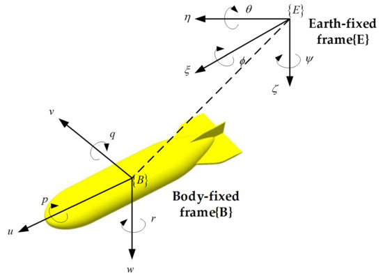
Figure 1.
Coordinate system of a UUV.
According to the structure of the UUV studied in the engineering application in our lab, there is no thruster to control the angular velocity in roll. Meanwhile, the rolling has little influence on the translational motion, so the roll speed can be ignored. Then, the kinematic and dynamic equations of UUVs can be described as:
where denotes the position and the attitude angle of the UUV in the Earth-fixed frame; is the velocity vector of the UUV in the body-fixed frame. is an unknown time-varying disturbance due to currents and waves. is the control input acting on the UUV in the body-fixed frame. In addition, is the transformation matrix; ,, and denote the inertia matrix, damping matrix, and the matrix of Coriolis and centrifugal terms, respectively. The structures of and are as follows:
The mathematical model of UUV is nonlinear and strong coupling. To solve the problem, the feedback linearization method is adopted to simplify the UUV model. The standard double integrator dynamic model can be described as:
The specific linearization process can be obtained from [28]. In (3), the external disturbances are not considered. Since the disturbance is unknown and nonlinear, no matter how the conversion is performed in the linearization process, the final form of disturbance is still unknown and nonlinear. Then, a modified linearization model is proposed in this paper as:
where , is the position and velocity of the in UUV formation with is the control input of . is an unknown time-varying disturbance.
Due to the complexity of the underwater environment, if faults occur to the leader in leader–follower method, the mission of UUV formation will not be able to be completed. To enhance the fault tolerance ability of the formation control, a virtual leader is introduced and defined as:
where is the position of the virtual leader, and is the velocity of the virtual leader. is a given bounded and time-varying function, and is a positive constant and . Define the error variable of the system as:
where is the desired relative position between and the virtual leader. The desired velocity of is the same as the velocity of the virtual leader, such that . Further, we assume and are bounded. Let
2.2. Graph Theory
Considering a multi-UUV system consisting of vehicles, we use the graph theory to model the information exchange among UUVs. Let the graph be an undirected graph, which consists of a node set , an edge set , and the adjacency matrix . The element denotes that the node can receive information from the node , otherwise . In addition, for all ,. Moreover, is undirected if . The collection of connected neighbors of is denoted as . The in-degree matrix is a diagonal matrix, where is the in-degree of node . Then the Laplacian matrix is defined as .
2.3. Artificial Potential Field
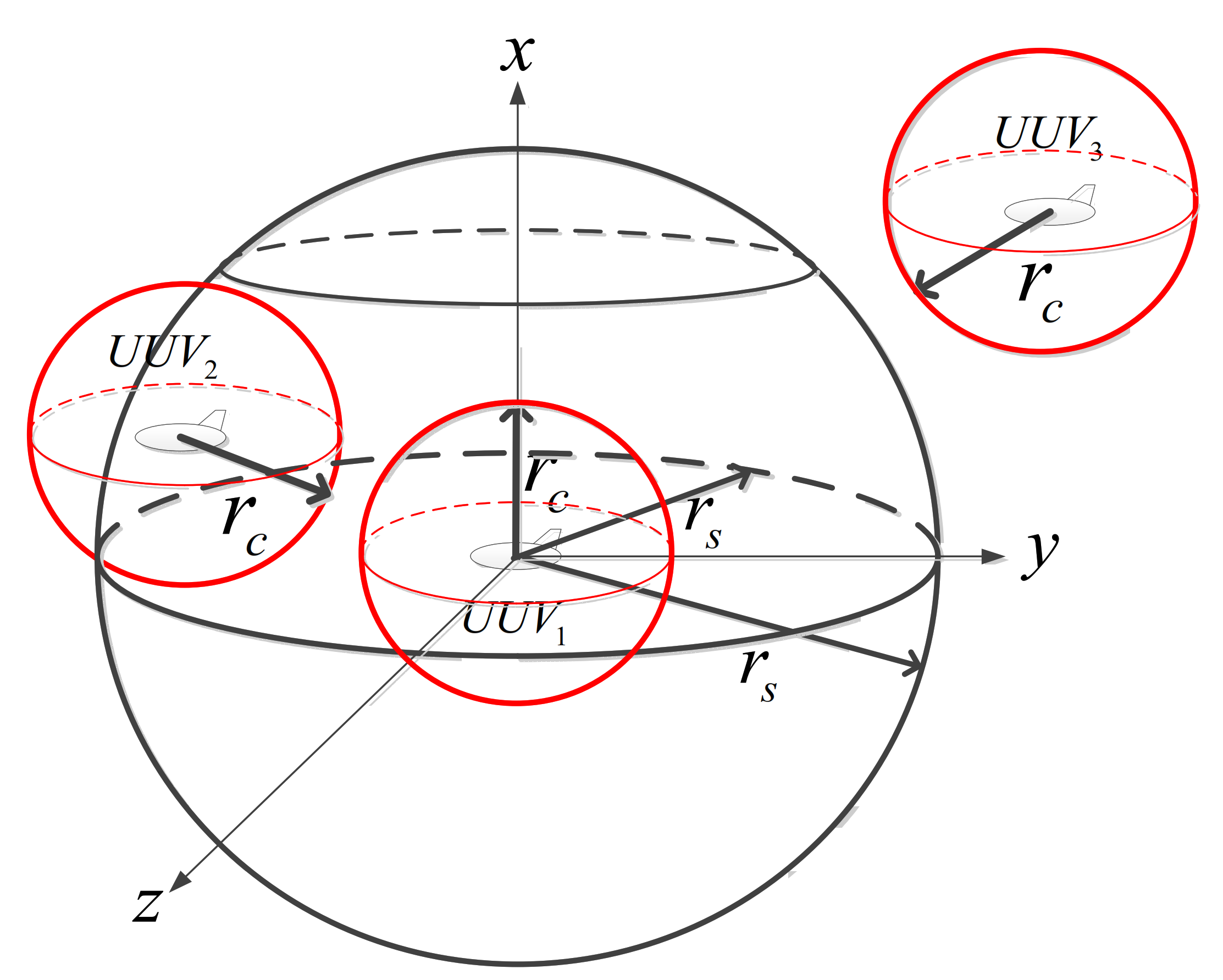
The APF method regards each UUV as a high-potential field. If any UUV is close to its neighbor, the repulsive force will repel the UUV away from other UUVs’ potential field. There are two advantages for collision avoidance by using the APF method. The first one is that the individuals of the multi-UUV systems can be separated from each other to avoid collisions. The second one is that fewer parameters need to debug, and the controller design is much simpler than other collision avoidance methods. In practical engineering, a UUV is a rigid body with volume instead of a particle. Then, we assume that each UUV has the same structure and define the collision sphere and the collision avoidance sphere of a UUV, as shown in Figure 2. The collision avoidance sphere is defined by the black sphere with safe radius . The collision sphere is shown by the red sphere with collision radius . We define as the distance between and , where . Shi [29] concludes that is a collision avoidance neighbor of UUVi while . When , collision occurs between and .

Figure 2.
The collision sphere and the collision avoidance sphere of UUVs.
To ensure that no collision occurs among the UUVs, an artificial potential function and an action function are defined as:
where is a design parameter. When is large enough, and , the potential function will tend to infinity. Thus, the repulsive force for collision avoidance is:
where denotes a negative gradient along .
Assumption 1.
The disturbance is time-varying and bounded. Then, there exists a positive constant, such that.
Assumption 2.
The velocity of UUVs and the virtual leader are not zero, e.g.,and. According to the characteristics of UUV, the velocity of UUVs is bounded,e.g.,and, whereandare positive constants.
Assumption 3.
At least one UUV can receive the information from the virtual leader,e.g.,, whereis the communication matrix between the virtual leader and followers. In addition, the communication between the UUVs is connected,e.g.,and.
Assumption 4.
The initial error in relative position and relative velocity of any two UUVs are bounded.e.g.,. andare positive finite values.
Lemma 1
([30]). Suppose and are all positive numbers; then, the following inequality holds:
Lemma 2
([31]). is a continuous function for any times, and the initial state of is bounded. If the inequality holds, for , then, we have the following inequality:
Lemma 3
([29]). and . If the Laplacian matrix of the undirected graph is irreducible, then the eigenvalues of the matrix are positive definite, e.g., .
3. Adaptive Formation Control Scheme Design
3.1. Adaptive Sliding Mode Disturbance Observer Design
In the process of performing underwater tasks, UUVs will be subject to environmental disturbances from ocean currents and waves. These disturbances are unknown and nonlinear. In this section, we design an adaptive sliding mode disturbance observer to estimate the disturbance . Firstly, an auxiliary state estimation error is defined as:
where is the auxiliary variable vector and its dynamic equation is designed as:
where is the switching term to be designed. Substituting (4) and (14) into the result of differentiating (13), it yields:
To guarantee that the system can deduce the sliding motion, we design the switching term as:
where , , and are all positive definite diagonal matrices. and are odd positive integers, and .
We design the Lyapunov function as follows:
Substituting (15) and (16) into the time derivative of , it yields:
According to Assumption 1, is bounded. Choose , such that . Thus,
According to Lemma 1, we have
Substituting (16) into (14), we obtain
where , and . According to [31], since , in the finite time, such that . Then, can be used to estimate the disturbance , i.e.,
where is the estimation of the .
3.2. Adaptive Formation Control with Collision Avoidance under Unknown Disturbances
The formation control scheme of the multi-UUVs are defined as:
where ,,, and are parameters to be designed; means that can receive the information from the virtual leader, and otherwise. The formation controller with collision avoidance under unknown disturbances is designed as
Theorem 1.
Under Assumptions 1–3, consider N UUVs with dynamics (1), control input (24) with adaptive sliding mode disturbance observer (16), and artificial potential function (8). If the control parameters are selected such that,, then the disturbance estimation error converges to zero in finite time, and ,holds, which means that (a) the tracking errors converge to a small neighborhood around zero; (b) collision avoidance can be guaranteed for each UUV.
Proof of Theorem 1.
We define the Lyapunov function as follows:
where represents the Kronecker product. Taking the time derivative of the Lyapunov function, we obtain
Substituting (23) and (25) becomes
We define that is the error between the real disturbance and the estimated disturbance. For an undirected graph, the repulsive forces between UUVs are equal and opposite in direction [32]. Therefore, . Then, we obtain
where . can approximate the disturbance in finite time; thus, . Let , then
Since ,, and are semi-definite. Thus, is negative semi-definite, which proves that is bounded. Then, the second derivative of is found as
where , and . Using polygon inequality, we obtain
By choosing the proper , the function is bounded. According to Assumption 1 and 4, we can see that the control law is bounded. This implies is bounded. Combining this with the fact that is bounded and is negative semidefinite, and applying the Barbalat’s lemma, we can obtain , as . is positive definite, from (29), which indicates . In addition, , which is only possible when all individual control parts become zero, and can estimate the disturbance [33]. Then, we can obtain
where can be obtained from Lemma 3. Therefore, . Then, the adaptive UUV formation system with disturbance achieves performance.
We define an energy function:
where denotes the relative position variable between the UUV and its collision avoidance neighbor UUV. Because all the UUVs in the formation have the same structure and characteristics of kinematic and dynamic, each UUV’s collision avoidance performance is analyzed in the same way. The specific proof can be obtained from [26]. Taking the time derivative of (29) yields:
From (30), it is easy to obtain , because of the disturbance observer we designed. The error terms and tend to zero. , , and are bounded. However, the potential function approaches infinity, if . Then, we can obtain the inequality by choosing the appropriate parameter as follows:
Then,
According to Lemma 2, we can obtain the following inequality
By designing the parameter , we have . Substituting it into (34), we obtain . Therefore, the UUV formations can avoid collisions among them by the proposed control law. □
4. Experimental Results and Simulation
To illustrate the effectiveness of the proposed algorithms, the simulation results are presented. The verification is mainly divided into two parts. The first one analyzes the effect of the sliding mode disturbance observer. The other part is about the effectiveness of the collision avoidance. The UUV formation consists of four UUVs in the simulation experiment, and is the virtual leader. Before showing the simulation results, some parameters used in the system are listed in Table 1.

Table 1.
Parameters.
The adjacency matrix and Laplacian matrix are
The initial velocities of the UUVs are designed as zero, and the initial position of the UUVs is given as
The position of the virtual leader is given as .
4.1. Disturbance Observer Simulation Result
Since the disturbance we considered is nonlinear and bounded, is given as:
The disturbance observer we designed is
The parameters are selected as , , , , and .
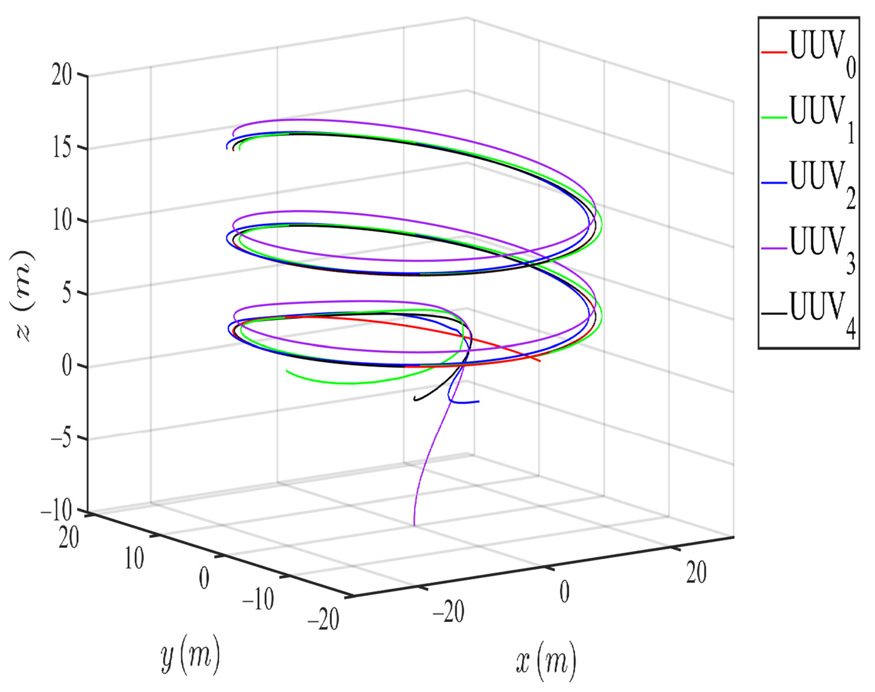
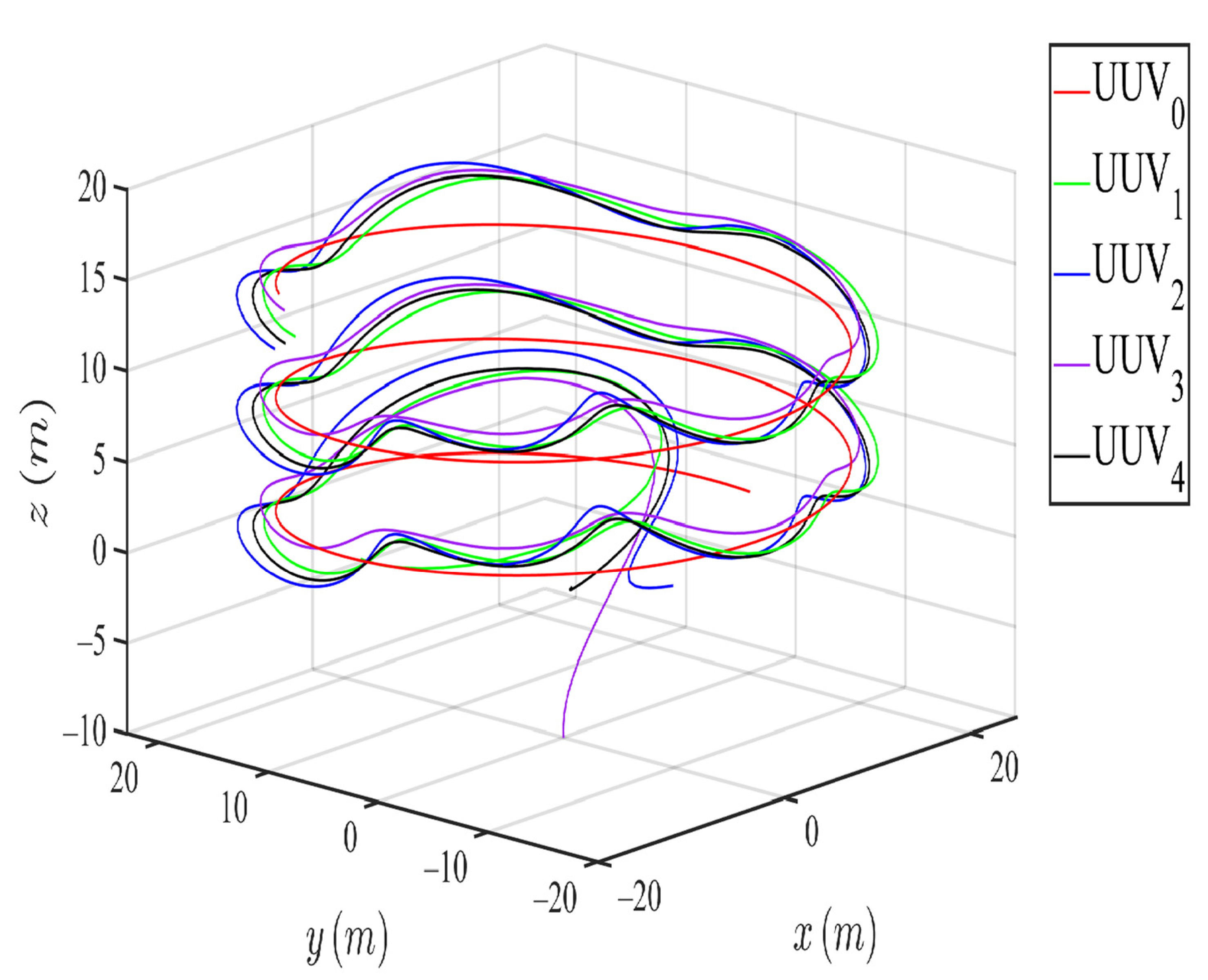
In this section, our goal is to illustrate the effectiveness of the sliding mode disturbance observer. Thus, the control law has included the part of collision avoidance in simulation. The virtual leader trajectory and the UUVs trajectories are plotted in Figure 3 to show the formation control performance; the initial and final position of the UUVs are also shown. The 3D trajectory in Figure 3 shows the controller with the disturbance observer. The tracking trajectory is smooth and steady. Figure 4 displays the 3D trajectory results from the controller without the disturbance observer. It is obvious that the tracking trajectory has jitter, and the disturbance has a great influence on the formation maintenance. The simulation results show that the adaptive sliding mode disturbance observer achieves good performance.

Figure 3.
3D trajectories of UUVs with disturbance observer.
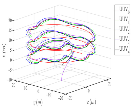
Figure 4.
3D trajectories of UUVs without disturbance observer.
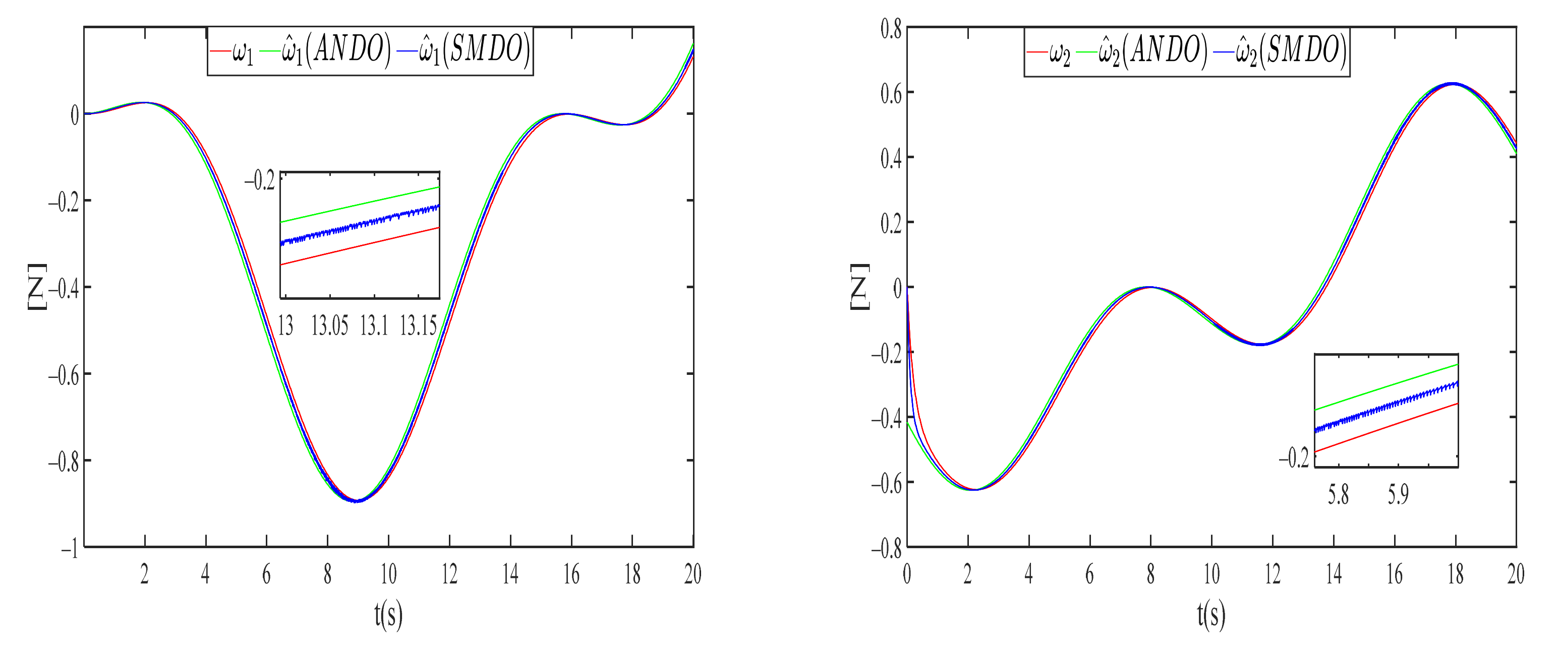
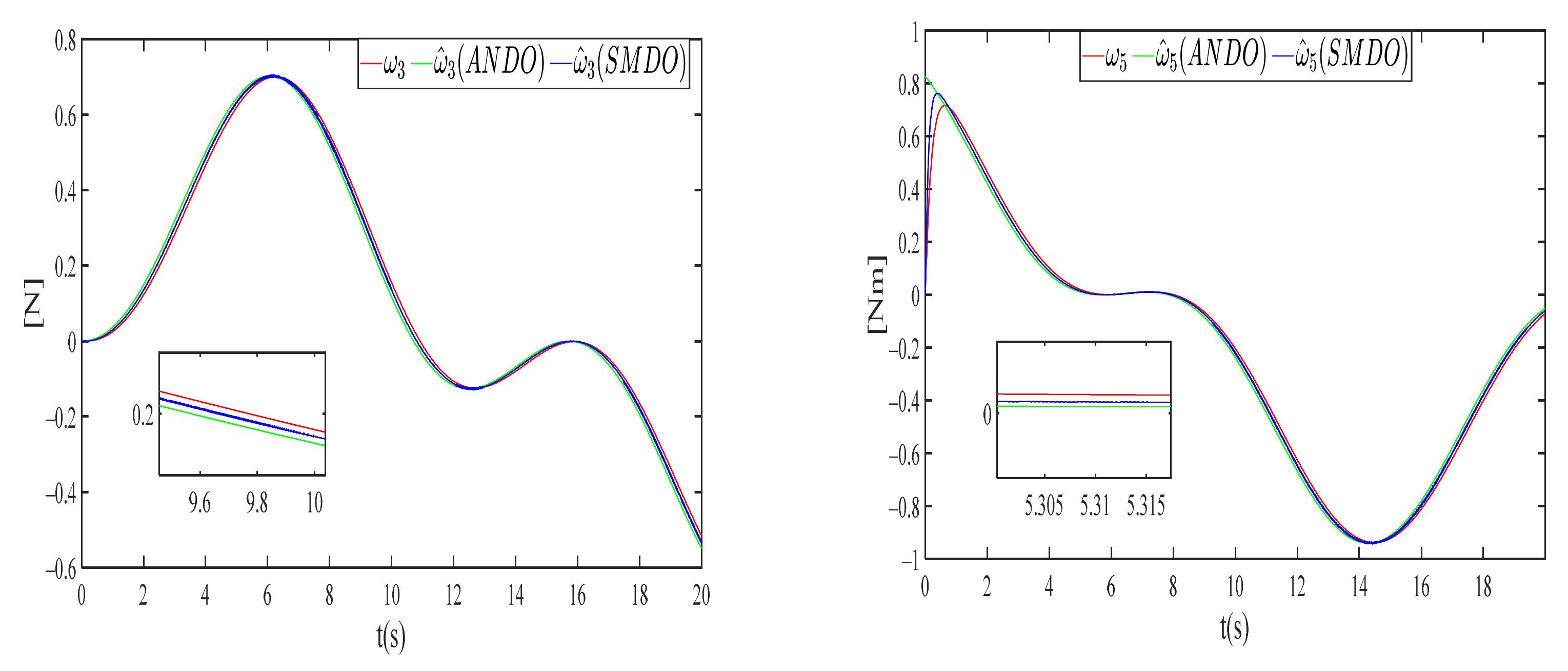
To verify the performance of the disturbance observer, an adaptive nonlinear disturbance observer (ANDO) proposed in [34] is compared with the observer proposed by us. The results of comparation are shown in Figure 5 and Figure 6. The red line is the real disturbance value curve. The blue line is the estimated value produced by the observer proposed in this paper. In addition, the green line is the estimation of the ANDO observer. From the enlarged views in Figure 5 and Figure 6, compared with the green line, the blue one is always closer to the red line. It means the estimation of SMDO is more precise than the ANDO. The SMDO achieves a better performance.
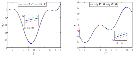
Figure 5.
The disturbance estimation comparation in and .
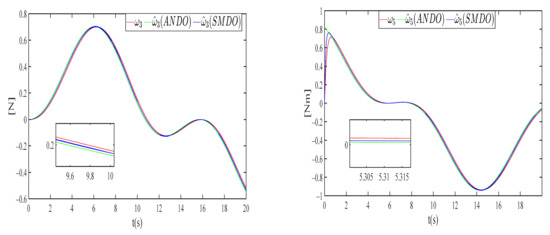
Figure 6.
The disturbance estimation comparation in and .
4.2. Collision Avoidance Simulation Result
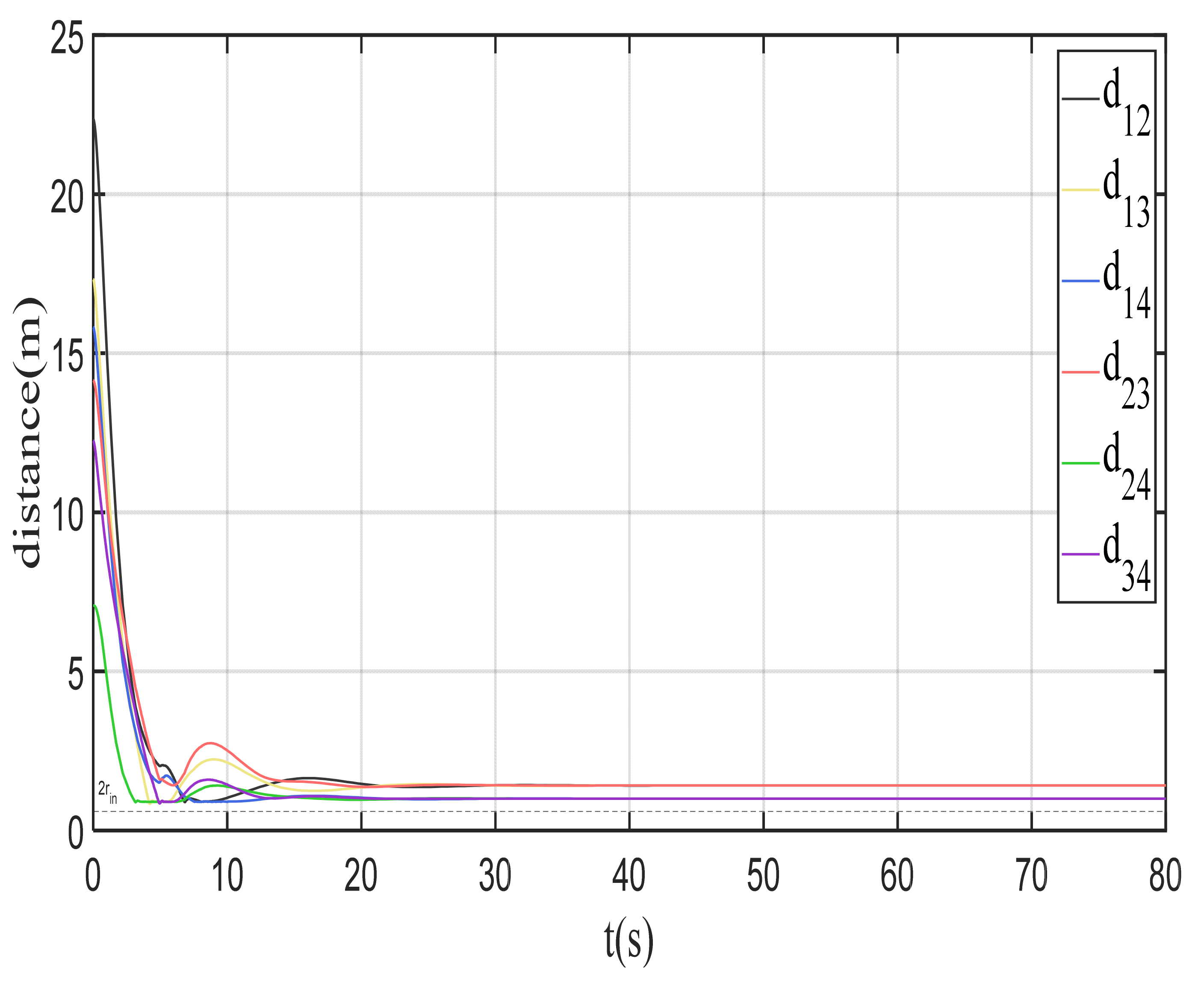
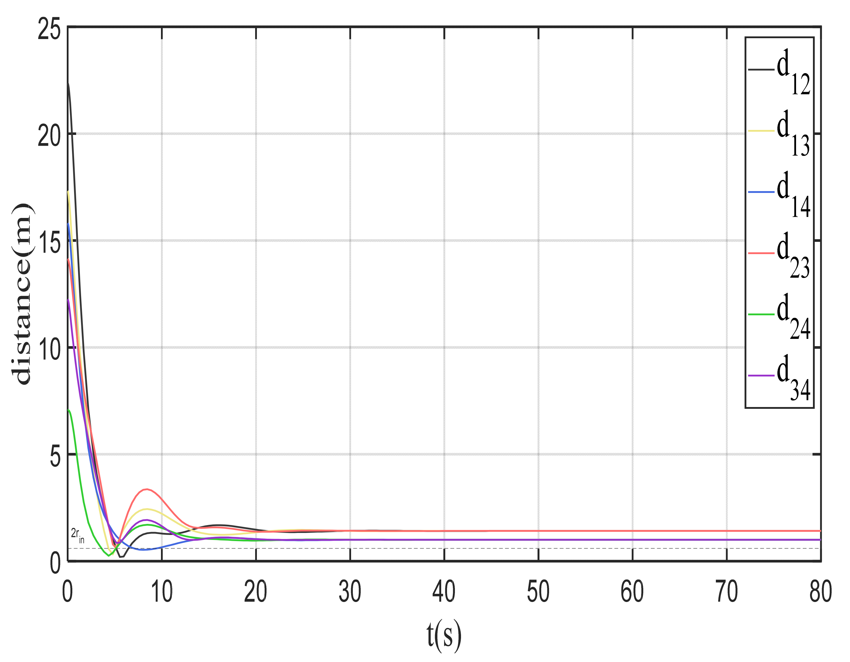
To show the performance of the controller of collision avoidance, we used the proposed disturbance observer to estimate the disturbance. Since the UUV will not stop after a collision, the difference of the 3D trajectories between the control law with collision avoidance and the controller without collision avoidance is small. So, the 3D trajectories are not displayed in this section. The distance between any two UUVs is more clearly to show the collision. The line is set at the bottom of the Figure 7 and Figure 8. If the distance , the collision occurs. Figure 7 shows the distance between any two UUVs of the formation with considering collision avoidance. There is no line under the line. Due to the spiral trajectory, there are some fluctuations in the distance between UUVs. It has no influence on the stability of system. Figure 8 shows the distance between any two UUVs of the formation without considering collision avoidance. It is obviously that collision occurs several times from 4 s to 6 s. The distance between UUVs is below . Without the collision avoidance control, the formation performance cannot be guaranteed.
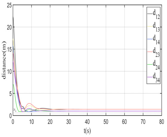
Figure 7.
The distance between any two UUVs of the formation with collision avoidance.
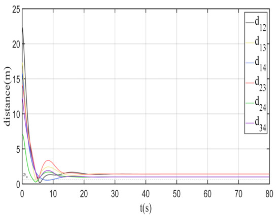
Figure 8.
The distance between any two UUVs of the formation without collision avoidance.
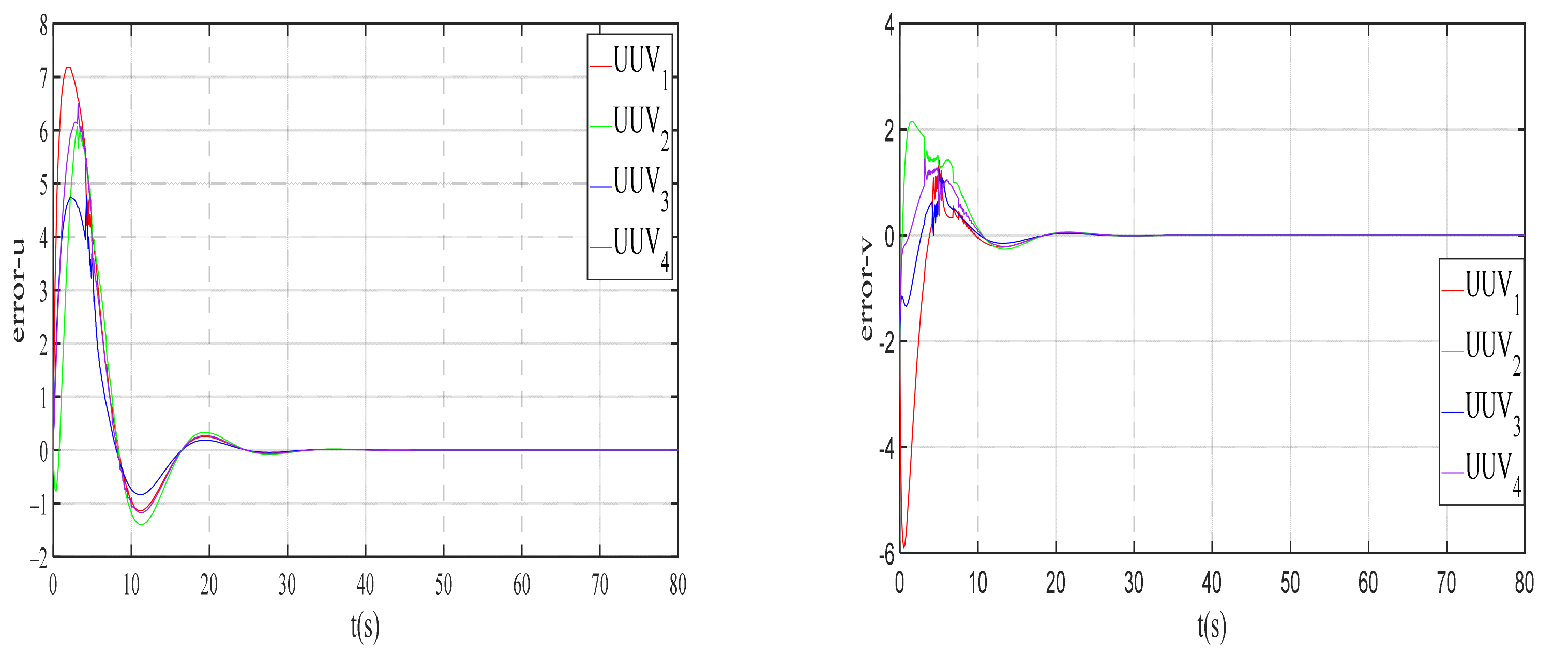
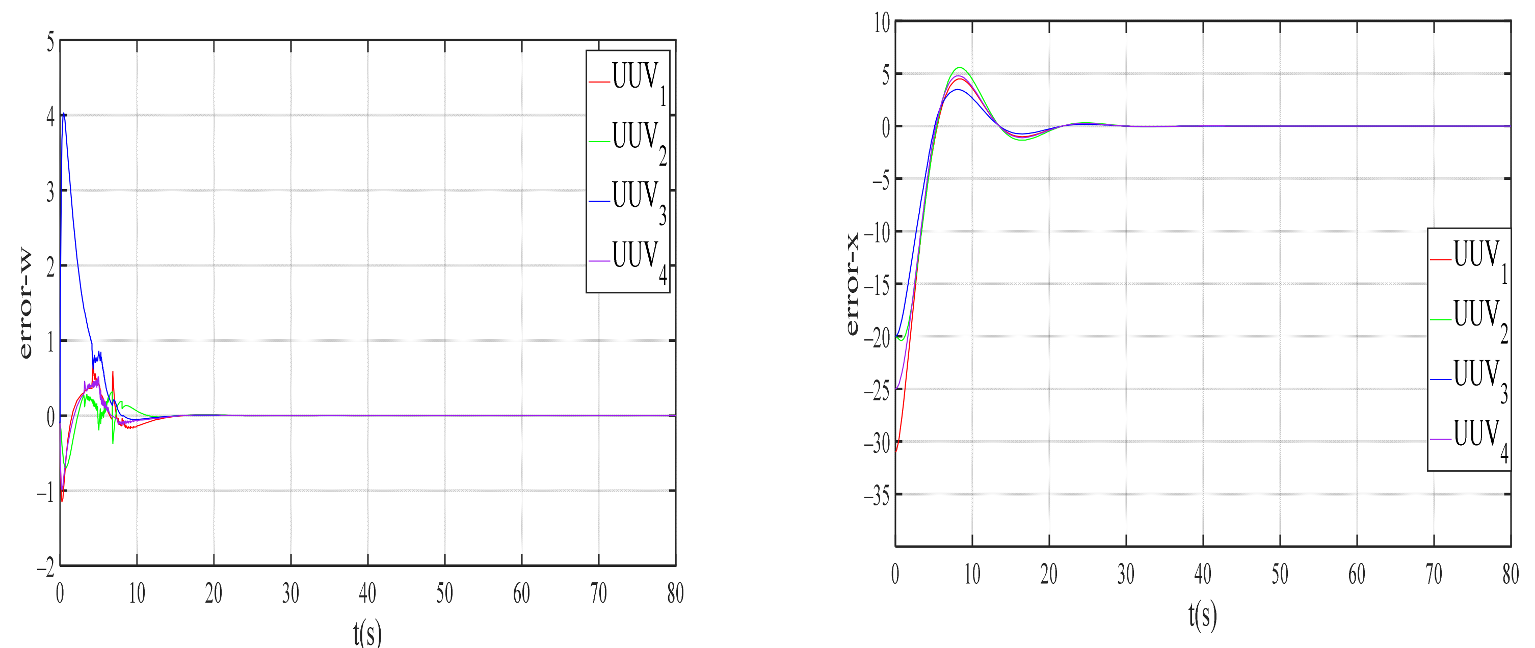
The position error and velocity error performance are validated as shown in Figure 9, Figure 10 and Figure 11. All the errors converge to zero in finite time, which means that the controller works satisfactorily and the system is stable. The simulation results show the four UUVs can track the virtual leader well without collision and maintain a good formation.
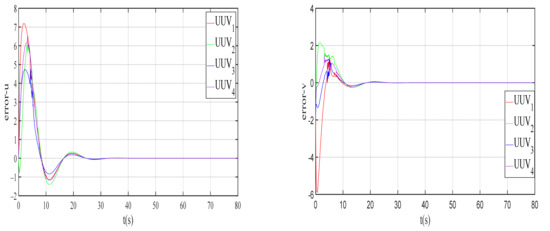
Figure 9.
Velocity errors of UUVs in and .
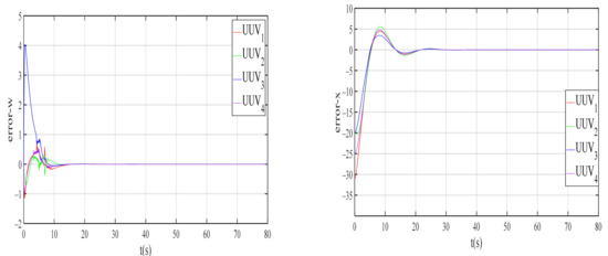
Figure 10.
Velocity errors of UUVs in , and position errors of UUVs in direction.
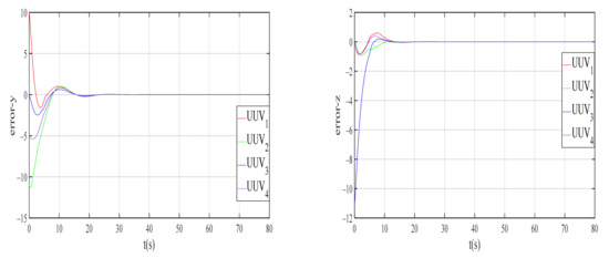
Figure 11.
Position errors of UUVs in and directions.
5. Conclusions
The adaptive formation control for multi-UUVs with collision avoidance under unknown disturbance was discussed. Graph theory was utilized to model the communications between UUVs. Feedback linearization was used to simplify the 5-DOF mathematical model. The overall structure of the control law was composed of a formation controller and a collision avoidance controller. The adaptive sliding mode disturbance observer was adopted to approximate the nonlinear and unknown dynamic disturbance term. By integrating the artificial potential field method into the virtual leader–following formation strategy, the problem of collision among UUVs was solved. The system stability was proven using the Lyapunov theory. Finally, we compared the proposed disturbance observer with the observer in another paper. The result shows the observer proposed in this paper performed better. The simulation results on formation control with collision avoidance have demonstrated the controller designed in this paper is valid and performs well. In the future, we will work on improving the observer to eliminate the jitter caused by the sliding mode and formation control subject to constraints.
Author Contributions
Conceptualization, A.J. and Z.Y.; methodology, A.J.; software, A.J. and C.L.; validation, A.J.; formal analysis, Z.Y.; investigation, A.J. and C.L.; resources, Z.Y.; data curation, A.J.; writing—original draft preparation, A.J.; writing—review and editing, Z.Y. and C.L.; supervision, Z.Y. All authors have read and agreed to the published version of the manuscript.
Funding
This research received no external funding.
Conflicts of Interest
The authors declare no conflict of interest.
References
- Liang, H.; Zhang, L.; Sun, Y.; Huang, T. Containment Control of Semi-Markovian Multiagent Systems with Switching Topologies. IEEE Trans. Syst. Man Cybern. Syst. 2019, 51, 3889–3899. [Google Scholar] [CrossRef]
- Liu, Y.; Shi, P.; Lim, C.-C. Collision-Free Formation Control for Multi-Agent Systems with Dynamic Mapping. IEEE Trans. Circuits Syst. II Express Briefs 2020, 67, 1984–1988. [Google Scholar] [CrossRef]
- Li, X.; Wen, C.; Chen, C. Adaptive Formation Control of Networked Robotic Systems with Bearing-Only Measurements. IEEE Trans. Cybern. 2021, 51, 199–209. [Google Scholar] [CrossRef] [PubMed]
- Zhou, K.-B.; Wu, X.-K.; Ge, M.-F.; Liang, C.-D.; Hu, B.-L. Neural-Adaptive Finite-Time Formation Tracking Control of Multiple Nonholonomic Agents with a Time-Varying Target. IEEE Access 2020, 8, 62943–62953. [Google Scholar] [CrossRef]
- Damasceno, B.C.; Xie, X. Deadlock-free scheduling of manufacturing systems using petri nets and dynamic programming. IFAC Proc. Vol. 1999, 32, 4870–4875. [Google Scholar] [CrossRef]
- Foumani, M.; Gunawan, I.; Smith-Miles, K. Resolution of deadlocks in a robotic cell scheduling problem with post-process inspection system: Avoidance and recovery scenarios. In Proceedings of the 2015 IEEE International Conference on Industrial Engineering and Engineering Management (IEEM), Singapore, 6–9 December 2015; pp. 1107–1111. [Google Scholar]
- Chen, W.; Wu, X.; Lu, Y. An Improved Path Planning Method Based on Artificial Potential Field for a Mobile Robot. Cybern. Inf. Technol. 2015, 15, 181–191. [Google Scholar] [CrossRef] [Green Version]
- Ghommam, J.; Saad, M. Backstepping-based cooperative and adaptive tracking control design for a group of underactuated AUVs in horizontal plan. Int. J. Control 2014, 87, 1076–1093. [Google Scholar] [CrossRef]
- Park, B.S. Adaptive formation control of underactuated autonomous underwater vehicles. Ocean Eng. 2015, 96, 1–7. [Google Scholar] [CrossRef]
- Huang, H.; Zhang, G.-C.; Li, Y.-M.; Li, J.-Y. Fuzzy sliding-mode formation control for multiple underactuated autonomous underwater vehicles. In Proceedings of the International Conference on Swarm Intelligence, Bali, Indonesia, 25–30 June 2016; pp. 503–510. [Google Scholar]
- Gao, Z.; Guo, G. Fixed-time sliding mode formation control of AUVs based on a disturbance observer. IEEE/CAA J. Autom. Sin. 2020, 7, 539–545. [Google Scholar] [CrossRef]
- Lu, Y.; Zhang, G.; Sun, Z.; Zhang, W. Robust adaptive formation control of underactuated autonomous surface vessels based on MLP and DOB. Nonlinear Dyn. 2018, 94, 503–519. [Google Scholar] [CrossRef]
- Park, B.S.; Kwon, J.-W.; Kim, H. Neural network-based output feedback control for reference tracking of underactuated surface vessels. Automatica 2017, 77, 353–359. [Google Scholar] [CrossRef]
- Franze, G.; Casavola, A.; Famularo, D.; Lucia, W. Distributed Receding Horizon Control of Constrained Networked Leader–Follower Formations Subject to Packet Dropouts. IEEE Trans. Control Syst. Technol. 2018, 26, 1798–1809. [Google Scholar] [CrossRef]
- Ajorlou, A.; Aghdam, A.G. A bounded distributed connectivity preserving aggregation strategy with collision avoidance property. Syst. Control Lett. 2013, 62, 1098–1104. [Google Scholar] [CrossRef]
- Sakai, D.; Fukushima, H.; Matsuno, F. Leader-Follower Navigation in Obstacle Environments While Preserving Connectivity without Data Transmission. IEEE Trans. Control Syst. Technol. 2018, 26, 1233–1248. [Google Scholar] [CrossRef] [Green Version]
- Dong, Y.; Su, Y.; Liu, Y.; Xu, S. An internal model approach for multi-agent rendezvous and connectivity preservation with nonlinear dynamics. Automatica 2018, 89, 300–307. [Google Scholar] [CrossRef]
- Wen, G.; Chen, C.L.P.; Liu, Y.-J. Formation Control with Obstacle Avoidance for a Class of Stochastic Multiagent Systems. IEEE Trans. Ind. Electron. 2018, 65, 5847–5855. [Google Scholar] [CrossRef]
- Park, B.S.; Yoo, S.J. An Error Transformation Approach for Connectivity-Preserving and Collision-Avoiding Formation Tracking of Networked Uncertain Underactuated Surface Vessels. IEEE Trans. Cybern. 2019, 49, 2955–2966. [Google Scholar] [CrossRef]
- Zhong, H.; Wang, Y.; Miao, Z.; Tan, J.; Li, L.; Zhang, H.; Fierro, R. Circumnavigation of a Moving Target in 3D by Multi-agent Systems with Collision Avoidance: An Orthogonal Vector Fields-based Approach. Int. J. Control Autom. Syst. 2019, 17, 212–224. [Google Scholar] [CrossRef]
- He, S.; Wang, M.; Dai, S.-L.; Luo, F. Leader–Follower Formation Control of USVs With Prescribed Performance and Collision Avoidance. IEEE Trans. Ind. Inform. 2019, 15, 572–581. [Google Scholar] [CrossRef]
- Huang, Y.; Liu, W.; Li, B.; Yang, Y.; Xiao, B. Finite-time formation tracking control with collision avoidance for quadrotor UAVs. J. Frankl. Inst. 2020, 357, 4034–4058. [Google Scholar] [CrossRef]
- Pan, L.; Bao, G.; Xu, F.; Zhang, L. Adaptive robust sliding mode trajectory tracking control for 6 degree-of-freedom industrial assembly robot with disturbances. Assem. Autom. 2018, 38, 259–267. [Google Scholar] [CrossRef]
- Chen, Z.; Yang, C.; Liu, X.; Wang, M. Learning control of flexible manipulator with unknown dynamics. Assem. Autom. 2017, 37, 304–313. [Google Scholar] [CrossRef]
- Yang, C.; Jiang, Y.; He, W.; Na, J.; Li, Z.; Xu, B. Adaptive Parameter Estimation and Control Design for Robot Manipulators with Finite-Time Convergence. IEEE Trans. Ind. Electron. 2018, 65, 8112–8123. [Google Scholar] [CrossRef]
- Nair, R.R.; Behera, L. Robust adaptive gain higher order sliding mode observer based control-constrained nonlinear model predictive control for spacecraft formation flying. IEEE/CAA J. Autom. Sin. 2016, 5, 367–381. [Google Scholar] [CrossRef]
- Hua, Y.; Dong, X.; Han, L.; Li, Q.; Ren, Z. Finite-Time Time-Varying Formation Tracking for High-Order Multiagent Systems with Mismatched Disturbances. IEEE Trans. Syst. Man Cybern. Syst. 2019, 50, 1–9. [Google Scholar] [CrossRef]
- Yan, Z.-P.; Liu, Y.-B.; Yu, C.-B.; Zhou, J.-J. Leader-following coordination of multiple UUVs formation under two independent topologies and time-varying delays. J. Cent. South Univ. 2017, 24, 382–393. [Google Scholar] [CrossRef]
- Shi, Q.; Li, T.; Li, J.; Chen, C.P.; Xiao, Y.; Shan, Q. Adaptive leader-following formation control with collision avoidance for a class of second-order nonlinear multi-agent systems. Neurocomputing 2019, 350, 282–290. [Google Scholar] [CrossRef]
- Yu, S.; Yu, X.; Shirinzadeh, B.; Man, Z. Continuous finite-time control for robotic manipulators with terminal sliding mode. Automatica 2005, 41, 1957–1964. [Google Scholar] [CrossRef]
- Wen, G.; Chen, C.L.P.; Dou, H.; Yang, H.; Liu, C. Formation control with obstacle avoidance of second-order multi-agent systems under directed communication topology. Sci. China Inf. Sci. 2019, 62, 1–14. [Google Scholar] [CrossRef] [Green Version]
- Pang, Z.-H.; Zheng, C.-B.; Sun, J.; Han, Q.-L.; Liu, G.-P. Distance- and Velocity-Based Collision Avoidance for Time-Varying Formation Control of Second-Order Multi-Agent Systems. IEEE Trans. Circuits Syst. II Express Briefs 2021, 68, 1253–1257. [Google Scholar] [CrossRef]
- Mondal, A.; Bhowmick, C.; Behera, L.; Jamshidi, M. Trajectory Tracking by Multiple Agents in Formation with Collision Avoidance and Connectivity Assurance. IEEE Syst. J. 2018, 12, 2449–2460. [Google Scholar] [CrossRef]
- Li, J.; Du, J.; Hu, X. Robust adaptive prescribed performance control for dynamic positioning of ships under unknown disturbances and input constraints. Ocean Eng. 2020, 206, 107254. [Google Scholar] [CrossRef]


Publisher’s Note: MDPI stays neutral with regard to jurisdictional claims in published maps and institutional affiliations. |
© 2022 by the authors. Licensee MDPI, Basel, Switzerland. This article is an open access article distributed under the terms and conditions of the Creative Commons Attribution (CC BY) license (https://creativecommons.org/licenses/by/4.0/).