Abstract
The water mass in the East China Sea (ECS) shelf has a complicated three-dimensional (3D) hydrologic structure. However, previous studies mostly concentrated on the sea surface based on the sparse in situ and incomplete satellite-derived observations. Therefore, the 3D interpolation technology was introduced for the reconstruction of hydrologic structure in the ECS shelf using in situ temperature and salinity observations in the summer and autumn of 2010 to 2011. Considering the high accuracy and good fitness of the radial basis function (RBF) methods, we applied the RBF methods to the in situ observations to completely reconstruct the 3D hydrologic fields. Other 3D interpolation methods and 2D methods were also tested for a comparison. The cubic and thin plate spline RBFs were recommended because their mean absolute error (MAE) in the 10-fold cross-validation experiments maintained the order of ~10−2. The 3D RBF reconstructions showed a reasonable 3D hydrologic structure and extra details of the water masses in the ECS shelf. It also helps evaluate regional satellite-derived sea surface temperature (SST). Comparisons between the interpolated and satellite-derived SST indicates that the large bias of satellite-derived SST in the daytime corresponds to weak mixing during low-speed wind and shows seasonal variation.
1. Introduction
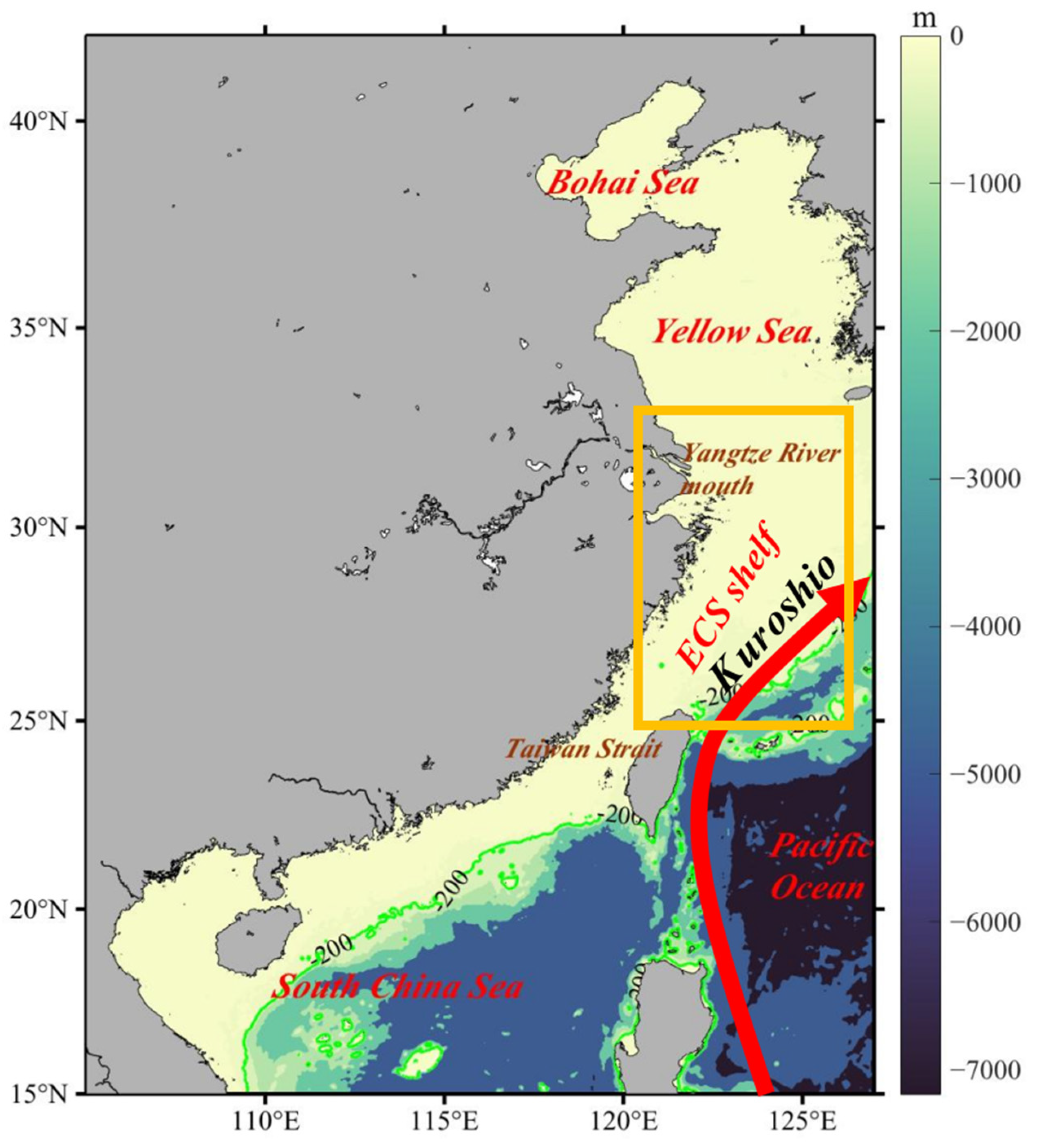
The East China Sea (ECS) is one of the largest marginal seas with significant sea–land interaction in the western Pacific (Figure 1). At the Yangtze River mouth, the isobaths of depth protrude outward in an arc. The distribution of hydrologic factors (temperature, salinity, etc.) in the ECS is affected by evaporation, precipitation, circulating currents, and also by the runoff from the Yangtze River into the sea. Previous research has shown that high-salinity water is located in the mid-shelf with less saline water in the inner shelf, forming a gradient parallel to the coast [1]. The ECS water mass is affected by the Yellow Sea circulation in the north, and the Kuroshio and its tributaries, which are manifested as a saline intrusion along with the warm water from the Taiwan Strait in the south. The mixture of the currents in the south is known as the Taiwan Warm Current [2,3,4]. At the same time, the Yangtze River enters the sea, extends eastward on the surface, and forms a new type of water by mixing with saline ambient water in the ECS shelf [5]. Overall, the distribution and properties of water mass in the ECS shelf are affected by these complex currents [6]. The ECS water mass has attracted extensive attention and there has been lots of research with slightly distinct results [7,8].
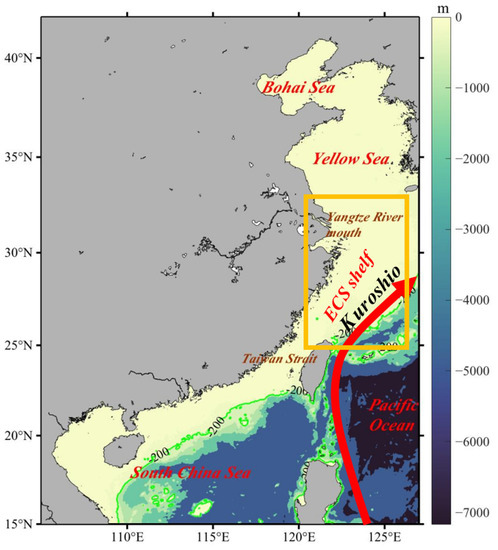
Figure 1.
Geographical location and bathymetry of the ECS shelf. The yellow box is the cruise field and the green line is the −200 m isobath.
With the continuous accumulation of data and the improvement of research technology, we have gained a deeper understanding of the ECS water mass. Most researchers mainly deal with the in situ and satellite-derived observations that could provide an accurate measurement of the sea surface conditions. For instance, Qiu et al. [9] used the in situ observations along with consecutive satellite data to investigate the fluctuations of the Kuroshio front in the ECS, Chang et al. [10] studied the wintertime variations of SST fronts in the Taiwan Strait using 10-year satellite SST images, and Yin and Huang [11] used satellite data of sea surface temperature (SST) to explore the short-term variation of the surface upwelling off northeastern Taiwan. Moreover, researchers also used various in situ and satellite observations to study deeper mechanisms in other areas under different ocean conditions. The variability and origin of surface chlorophyll-a concentration under different climate conditions in the Malacca Strait, the South Java Coast, the Southern California Bight, the Indonesian Maritime Continent, and the South China Sea were studied using multiple remote sensing observation platforms and Argo observations [12,13,14,15,16]. Isa et al. [17] used the Advanced Very High-Resolution Radiometer SST in the Malacca Strait to study the long-term trends and impacts of the El Southern/Oscillation and Indian Ocean Dipole. Mandal et al. [18] used different kinds of data (e.g., Argos and satellite datasets) to evaluate different phases of the cyclonic storm ROANU along the western Bay of Bengal.
Various data play an important role in explaining different ocean phenomena and studying the changes in different scenarios. However, affected by the conditions in the real sea, the observed data are often not satisfactory. For example, the satellite datasets could only provide effective surface data and there also exist missing pixels due to the cloud cover and coastline interference. Interpolation technology is often used to help make up for their defects [19]. The two-dimensional (2D) interpolation schemes are usually used for the reconstruction of sea surface data such as the Forel–Ule index [20]. In this paper, the conductivity-temperature-depth (CTD) data are used for a complete three-dimensional (3D) reconstruction of the hydrologic factors in the ECS shelf. Due to the inherent limitation of the cruise surveys, the temperature and salinity data measured by the ship-based CTD are sparse and discrete, raising a need for interpolation. We could reconstruct the data of each layer through 2D interpolation, but unfortunately, there are only a few in situ observations in one layer. In this situation, the 2D interpolation could not provide a satisfactory result. In addition, the topography variability of the ECS shelf leads to the uneven distribution of in situ observations in each layer, that is, the number of measured points in the shallow water is larger than that in the deep part so that the 2D interpolation would perform differently at different depths. Under these circumstances, accurate interpolation results could not be accessible. For the coherent 3D temperature and salinity fields in the ECS, the 2D interpolation results without considering the vertical information in the calculation could hardly reflect the geophysical distribution and complicated phenomena. Hence, for a higher spatial resolution, more accurate interpolation results, and less computational cost, we propose the 3D interpolation scheme. So far, many 3D interpolation methods have been tested in a relatively comprehensive way in the reconstruction of the diapycnal diffusivity in the South China Sea [21]. However, the 3D interpolation methods are not widely used in oceanography yet.
In addition, the 3D interpolation could provide a more accurate result in surface data reconstruction. SST is a significant index to investigate large-scale phenomena and local variability and hence is important for the studies in the ECS shelf affected by complex monsoon conditions. The satellite-derived SST datasets have been verified in a wide range of waters, such as the western North Pacific, the South China Sea, and the north Persian Gulf [22,23,24]. Spatially interpolating the in situ observations onto the grids of satellite measurements could provide more reliable matchups to assess the performance of satellite-derived SST. Therefore, spatial interpolation techniques are essential for estimating hydrologic variables for unsampled locations. The 3D interpolation methods can integrate the information of vertical direction, which has obvious advantages compared with the 2D interpolation methods. Therefore, it is more convincing for using the 3D interpolation results to evaluate satellite-derived SST.
In terms of multidimensional scattered data completion, there are several methods available. The inverse distance weighted (IDW) method [25], the Chebyshev polynomials fitting (CPF) method [26], and the radial basis functions (RBF) method [27] have been widely used in many fields. Especially as an effective interpolation method of the high dimensional interpolation, the accuracy of the RBF methods is determined by the matching degree between the distribution of in situ observations and the type of RBF. The real distribution is hard to obtain, and therefore, we apply the 10-fold random cross-validation experiments [28] to choose the optimum interpolation method to interpolate the in situ observations. The main purpose of the paper is to select the appropriate interpolation scheme, obtain the complete 3D spatial hydraulic structure in the ECS shelf, analyze its water mass composition, and evaluate the satellite-derived SST.
The paper is organized as follows. The data are described in detail in Section 2. In Section 3, the 3D RBF interpolation method is introduced and compared with several other interpolation methods. The reconstruction results, analysis of the results and evaluation of satellite-derived SST are shown in Section 4 while Section 5 gives the summary.
2. Data
2.1. In Situ Observations
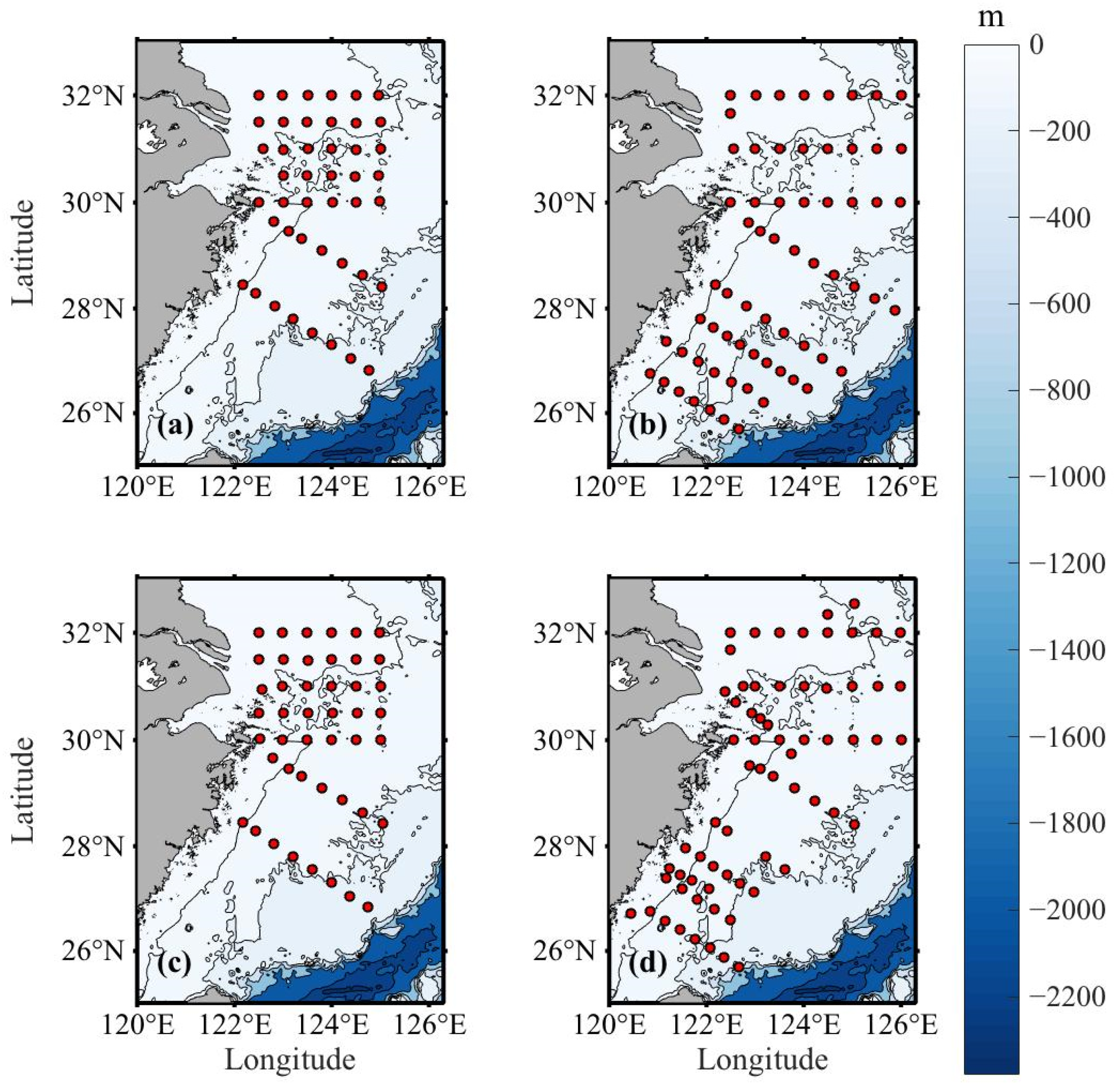
Historical hydrologic data used in this study were collected from four field surveys during the summer and autumn in 2010 and 2011. Figure 2 shows that some stations are close to each other. However, distinct scattered points are needed to obtain a unique interplant when using the RBF method. Consequently, for the pair of stations between which the distance is smaller than ~20 km, we will screen out one of them from the data set. The detailed cruise period and the number of stations used in the paper are listed in Table 1. Temperature and salinity data were measured by the ship-based CTD (SBE911). The in situ observations cover the ECS shelf around 25° N–32° N, 120° E–126° E. The horizontal distribution of the stations is shown in Figure 2, which shows that the stations are mostly located at a depth shallower than −200 m. The data recorded within one month are used as a proxy of the corresponding season: June for summer, and October and November for autumn.

Figure 2.
Processed cruises station distributions in the ECS shelf. The red dots show the locations of stations, and the black lines present the −50 m, −100 m, −200 m, −500 m, −1000 m, and −2000 m isobaths. (a) Summer (June) 2010; (b) Summer (June) 2011; (c) Autumn (November) 2010; and (d) Autumn (October) 2011.

Table 1.
The number of the stations and observations included in the paper.
2.2. MODIS SST Data
We use the satellite-derived SST from the Moderate-resolution Image Spectroradiometer (MODIS) on board Auqa that could cover the global earth in one to two days. The in situ observations are used as a proxy to represent one season, and we also use the monthly data in 2010 and 2011 from the product with thermal-infrared (derived from bands 31–32, i.e., 10.8–12.3 μm) SST. We use the MODIS SST Level 3 product in daytime that is produced by the NASA Goddard Space Flight Center’ s Ocean Data Processing System (https://oceancolor.gsfc.nasa.gov/, (accessed on 15 April 2022)).
3. Methodology
Interpolation methods are in great demand in the fields of oceanography and meteorology. Several widely used methods are applied to reconstruct the integrated hydrologic structure. Our experiment is only aimed at interpolating the data spatially for different seasons separately. The 2D interpolation methods are also tested as comparison. The results are shown in Section 3.3, which show the best RBF for reconstruction, while the 3D IDW and CPF methods are implemented as comparison. The formula of the 3D IDW method and the 3D CPF method (Equations (5) and (6)) are similar to Guo et al. [21].
3.1. The RBF Method
The radial basis functions (RBF) method is a precise interpolation method and will be applied to this multivariate scattered data interpolation problem. The RBF method is effective and relatively accurate when dealing with unevenly and sparsely distributed n-dimensional observations [29]. It is presented as the following form (n = 3 in our paper):
where is the number of data points, , , and represent horizontal coordinates and vertical coordinates, respectively, is the input vector, is set as the Euclidean norm in our paper, means the temperature or salinity distribution field, is the RBF, and are the coefficients. The coefficients could be obtained by solving linear algebraic equations (Equation (2)) [30] with the in situ observations :
where , , and
One of the most attractive advantages of the RBF method is the uniqueness of the interpolant under rather mild conditions. The Equation (2) could be simplified as for some kinds of RBFs, since the RBF method yields the unique interpolant if and only if the matrix is non-singular. It could guarantee the uniqueness if the RBFs are chosen as Gaussian, multiquadric, or linear functions. While using the thin plate spline and the cubic function, the uniqueness needs to be satisfied by either changing to the Equation (2) or giving stronger restrictions to the datasets [30]. In practical application, the latter could be rarely realized. As a result, the last four terms of the coefficients vector are added to guarantee the uniqueness of the interpolant of all the RBFs used in this paper [31]. Moreover, their effectiveness in the scattered data interpolation depends on their easily adjustable smoothness and powerful convergence properties [32].
However, the interpolation results are under the influence of the types of RBFs, since the RBFs indicate different trends. Hence, there exists a risk that an improper RBF is chosen. The RBFs mentioned above are listed as: (1) (linear), (2) (cubic), (3) (thin plate spline), (4) (multiquadratic), and (5) (Gaussian), where is the distance (Euclidean distance or other distances) between two points, and represents the reciprocal of the critical radius for multiquadratic and Gaussian functions and is set as approximate average distance between two adjacent nodes in our test (shown in Equation (4)). Generally, these RBFs correspond to the linear, cubic, and almost quadratic, as well as exponential decay trends [29]. Due to the stable features of the temperature and salinity fields, the RBF (1) to (4) are tested in our paper.
The basis for choice is the prior knowledge of the data set (the real distribution of temperature and salinity) that could not be obtained beforehand. Therefore, we carry out the 10-fold random cross-validation experiments to decide which RBF is the optimum for our reconstruction. To accomplish the numerical test, the data set is randomly divided by record. All the in situ observations are divided into 10 disjoint subsets randomly, each containing of the data. We randomly select one group every time for one calculation process. The picked group is set as a test set while the remaining groups are used for interpolation. The calculation error of the interpolation will indicate the effect of different methods. The 10-fold cross-validation experiments are repeated 10 times to make sure the stability and accuracy of the results and other interpolation methods will also be tested in this way.
3.2. The 3D IDW Method and the 3D CPF Method
The 3D IDW method is one of the most common interpolation methods in data analysis. The surrounding points contribute different weights to the interpolated point, which are inversely proportional to the distances between the interpolated points and surrounding points. The formula is presented as follows:
where , is a 3D vector and is still the Euclidean norm.
The 3D CPF method is another popular fitting method using the orthogonal polynomials and the formula is shown in Equation (6).
3.3. Experimental Results
Different interpolation methods are applied to reconstructing the in situ observations. In order to quantify their effectiveness, the 10-fold random cross-validation scheme is carried out, and the criterions are formulated by the mean absolute error (MAE) and the mean relative error (MRE), which are shown as follows:
where and represent the interpolated and measured values, respectively, and is the number of points in one test set. We use the Miller projection (a kind of improved cylindrical map projection) to convert longitude and latitude coordinates into X–Y coordinates in a plane for interpolation process and the depth coordinates have no change. We calculate the change rate of each pair of points. The percentage of the pairs whose change rate is located within a certain range of temperature and salinity calculated for 2011 cruises is shown in Table 2. More than 50% pairs of points are located within the listed range in Table 2. This means that the change rate in vertical direction is actually 2–4 orders of magnitude higher than that in the horizontal direction. However, the value of the distances between two points is reduced to of the actual distance after the projection and the “change rates” (the quotations mean the change rate after the Miller projection) is correspondingly times higher. Therefore, when the calculation process is going on, the “change rate” in the horizontal direction is ~2–4 orders higher than that in the vertical direction. Through some tests, the change rates of each dimension are kept consistent as far as possible so that better results can be obtained. Hence, during the calculation process we raise the weight of the change rate in the vertical direction by after tests. in Equation (1) is replaced by while and in Equation (1) are the projected coordinates in the actual interpolation.

Table 2.
Percentages of pairs of points whose change rates are within the specific range for temperature and salinity in horizontal and vertical directions for cruises in 2011.
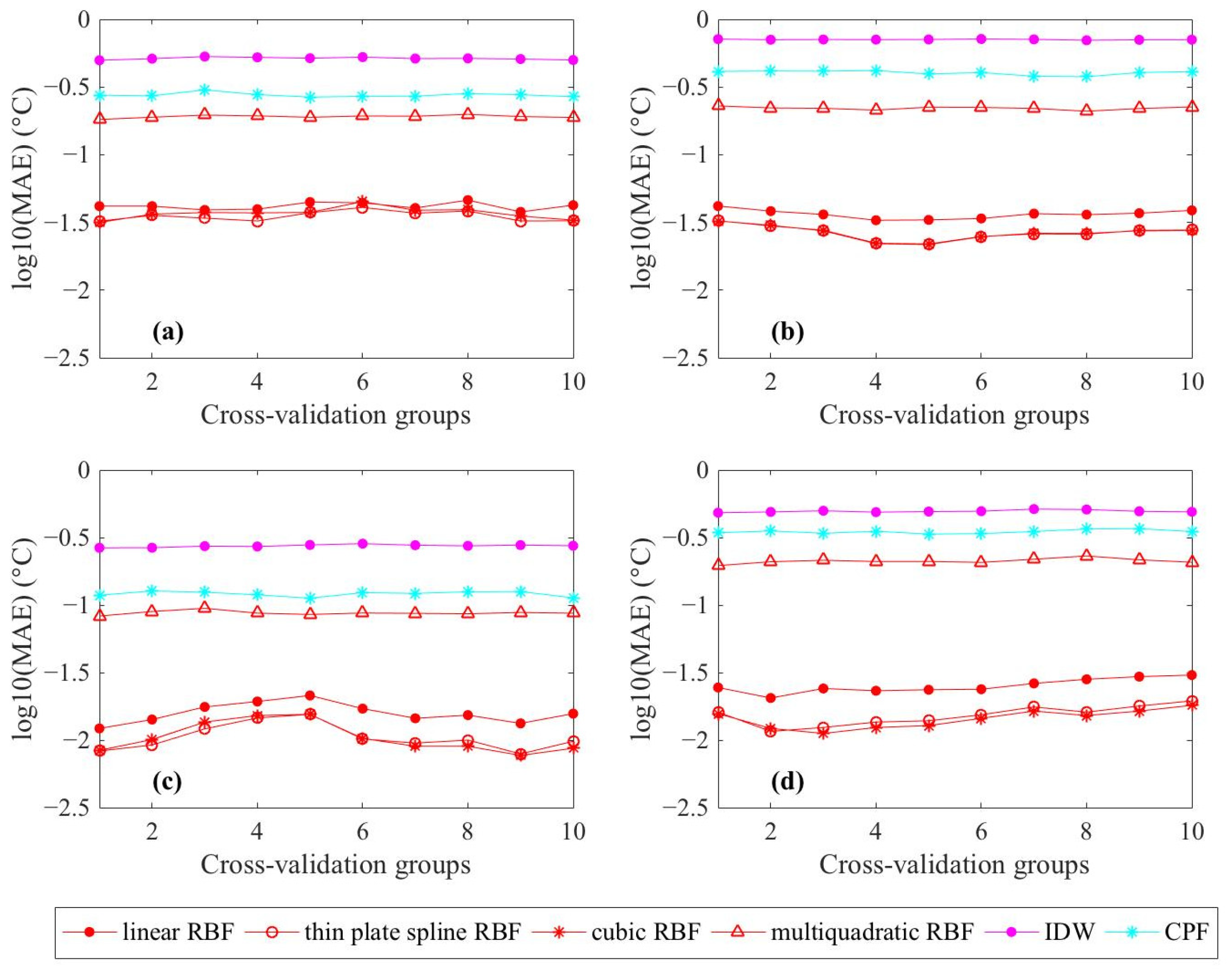
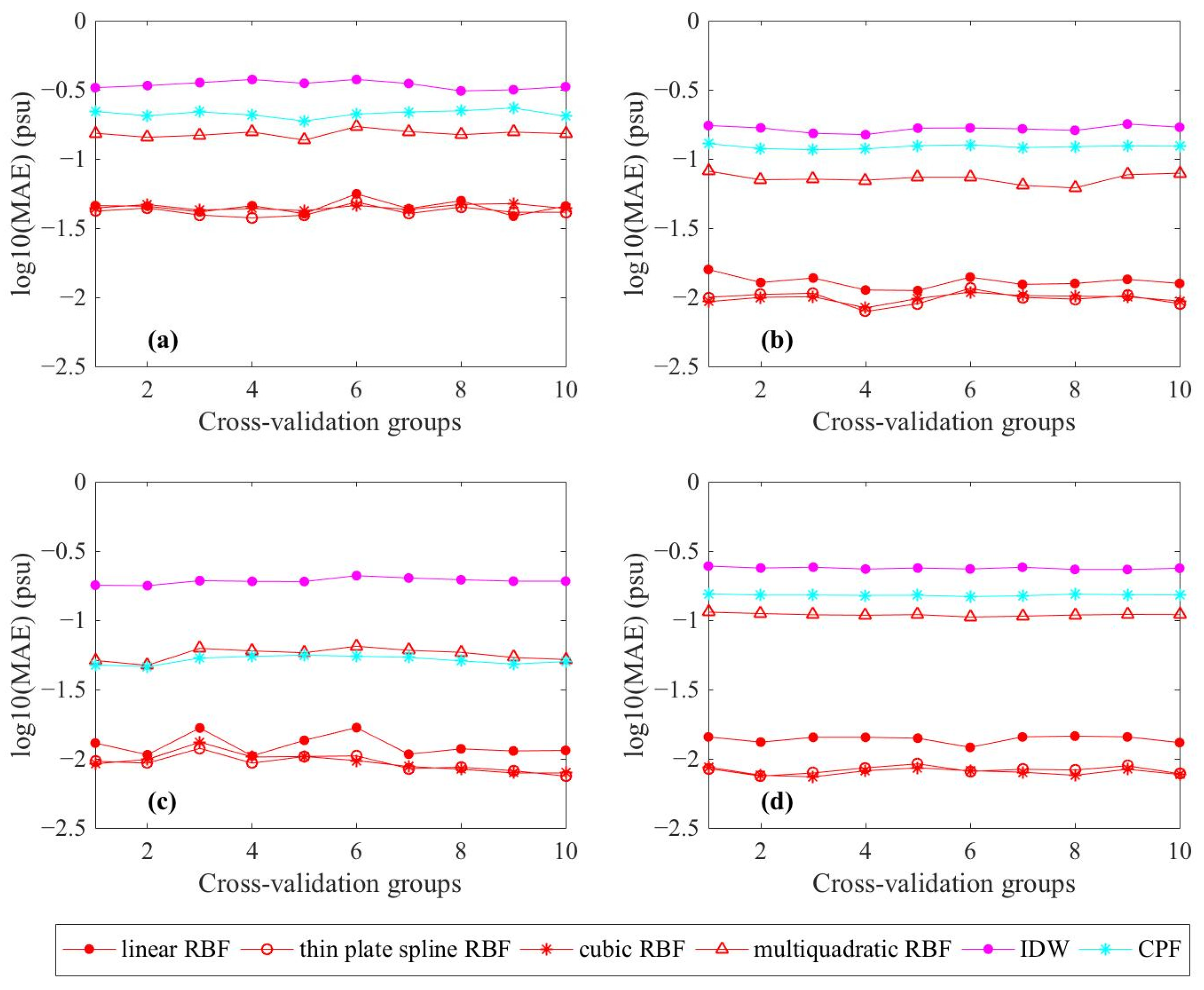
We test different cruises with the 10-fold cross-validation experiments and the results are shown in Figure 3 and Figure 4. Considering that the MAEs of different methods are too low to distinguish from each other, we present the log10(MAE) to enlarge their differences. Due to the smaller variation range of salinity in the ECS shelf, the errors of salinity are slightly lower than that of temperature. We could see obvious advantages of the RBF method. In most groups, the MAEs of linear, thin plate spline, and cubic RBFs are in the order of ~10−2 in each group and they are always one order of magnitude lower than others (~10−1). In addition, the MAEs of thin plate spline and the cubic RBF methods are lower than the linear RBF method in most situations.
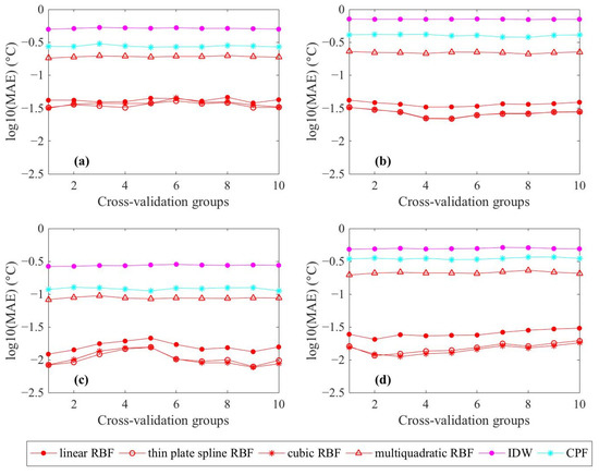
Figure 3.
The log10(MAE) of each method in the 10-fold cross-validation experiments for temperature interpolation. (a) Summer 2010; (b) Summer 2011; (c) Autumn 2010; and (d) Autumn 2011.
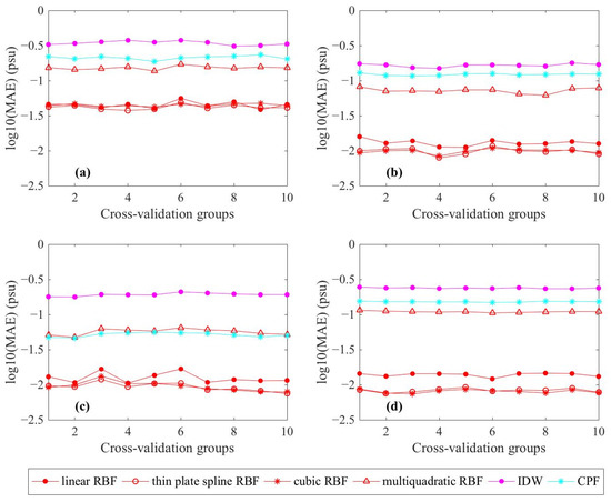
Figure 4.
The log10(MAE) of each method in the 10-fold cross-validation experiments for salinity interpolation. (a) Summer 2010; (b) Summer 2011; (c) Autumn 2010; and (d) Autumn 2011.
MREs (the average of 10 tests) indicate the same conclusion (Table 3 and Table 4). The average MREs are obviously small for the RBF method of the linear, thin plate spline, and cubic functions. The error can be reduced to ~1 to 2 order of magnitudes lower than other methods and the thin plate spline and the cubic RBF have the smallest errors. The RBF methods perform better in terms of accuracy and stability under different conditions. The experimental results with a different data set of the four cruises support this conclusion without exception. Furthermore, the use of different target values (temperature and salinity) do not make any difference about the results.

Table 3.
The average MREs of different interpolation methods with in situ temperature.

Table 4.
The average MREs of different interpolation methods with in situ salinity.
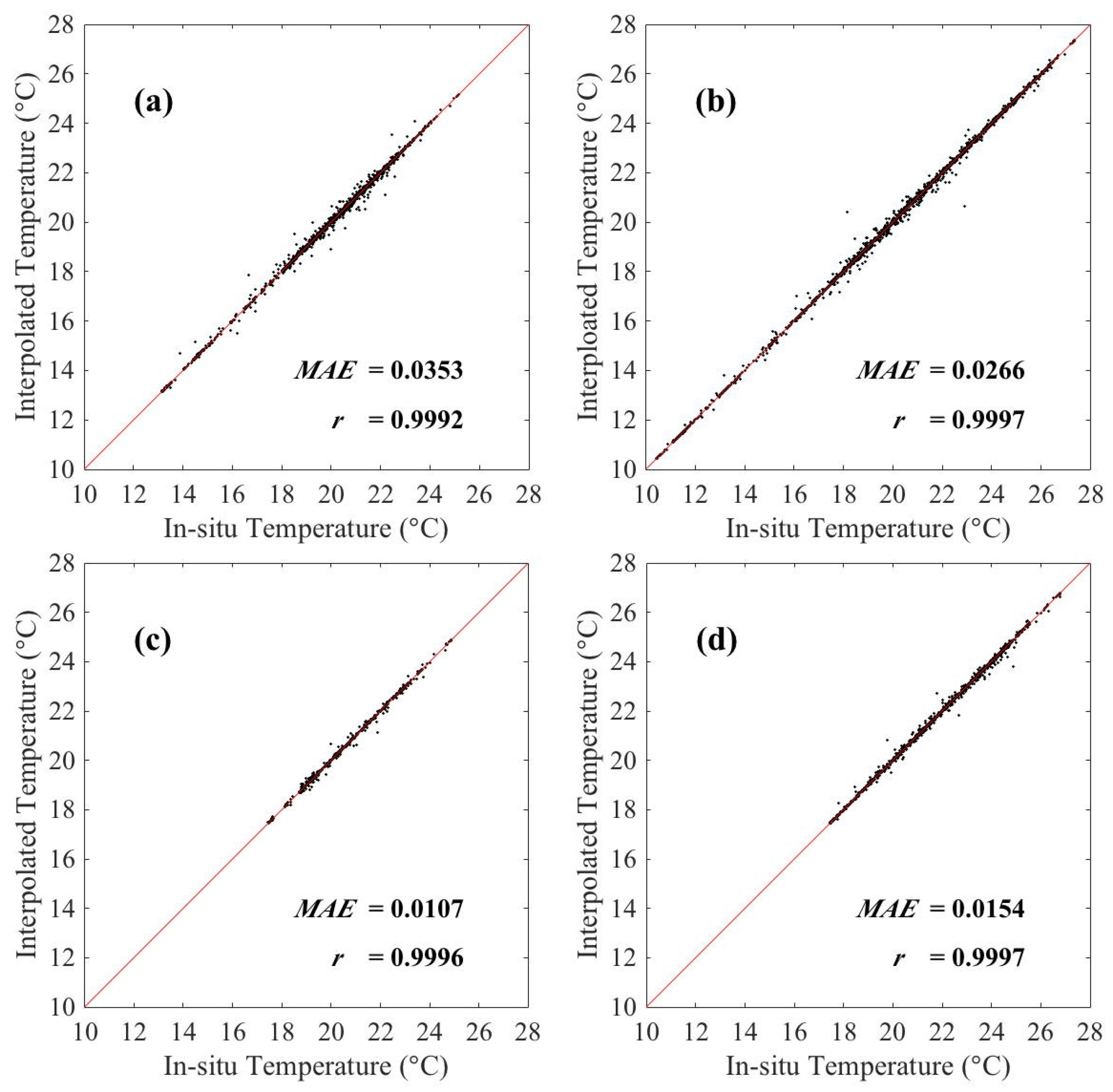
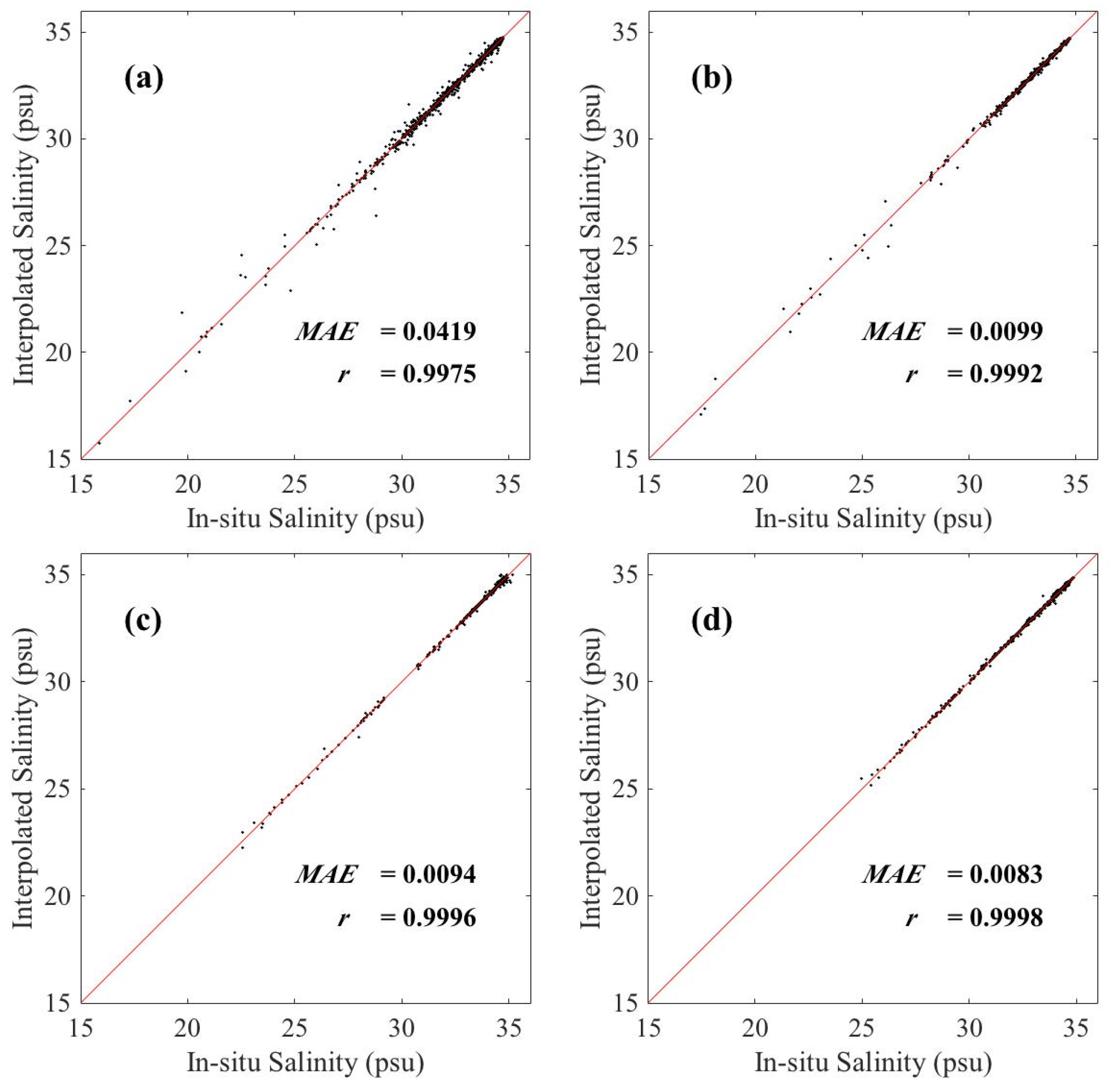
The scatterplots of the matchups between the interpolated and in situ values (all the interpolations at the positions of in situ observations in 10 test groups are considered) are presented in Figure 5 and Figure 6. Generally, most points are close to the 1:1 line for the entire ECS shelf and the bias calculated following Equation (9) (where is the total number of the matchups) is on the order of ~10−4 for all situations. Quantitatively, the correlation coefficients and MAE show that the RBF reconstructions have a good agreement with the in situ data in all conditions. The MAEs of all 10 test groups are in the order of ~10−2 in Figure 5 for all the conditions while the interpolated results in summer are slightly worse. The same condition occurs in salinity interpolation. The MAEs of all the in situ observations are smaller than the order of 10−2 except that in summer 2010 (Figure 6a), with MAE equaling to 0.0419 psu. It is noticed that the larger biases are mostly distributed in the area with a low salinity, which is near the Yangtze River mouth through the matchups in Figure 6a,b. It implies that the gradient distributions of the target values possibly have an essential impact on the interpolated results.
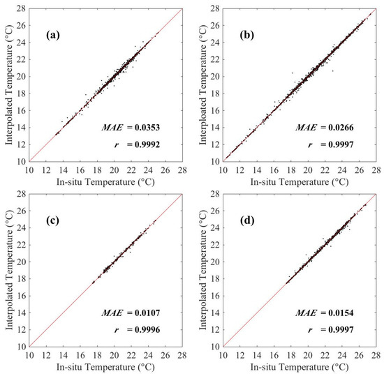
Figure 5.
Scatterplots of the matchups between the interpolated and in situ temperature. The red line is the 1:1 line and is the correlation coefficient. (a) Summer 2010; (b) Summer 2011; (c) Autumn 2010; and (d) Autumn 2011.
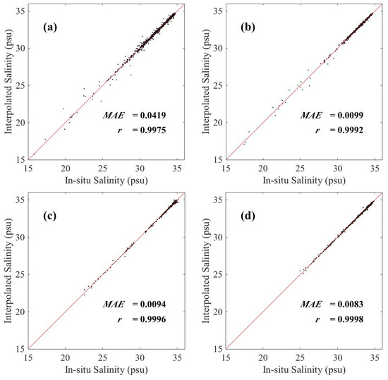
Figure 6.
Scatterplots of the matchups between the interpolated and in situ salinity. The red line is the 1:1 line and is the correlation coefficient. (a) Summer 2010; (b) Summer 2011; (c) Autumn 2010; and (d) Autumn 2011.
We notice that the MAEs present some difference for different cruises while the similar results are also revealed in scatterplots of the matchups. For the temperature, the MAEs in the summers of 2010 and 2011 are slightly larger than that in autumn. For instance, the average MAE of the thin plate spline RBF method in summer 2010 is 0.0353 °C while it is 0.0154 °C in autumn 2010. For salinity, the MAEs in summer 2010 are larger than that in other cruises, which is also reflected in Figure 6 with a more scattered distribution of the matchups. The average MAE of the thin plate spline RBF method in summer 2010 is 0.0419 psu while it is 0.0094 psu in autumn 2010.
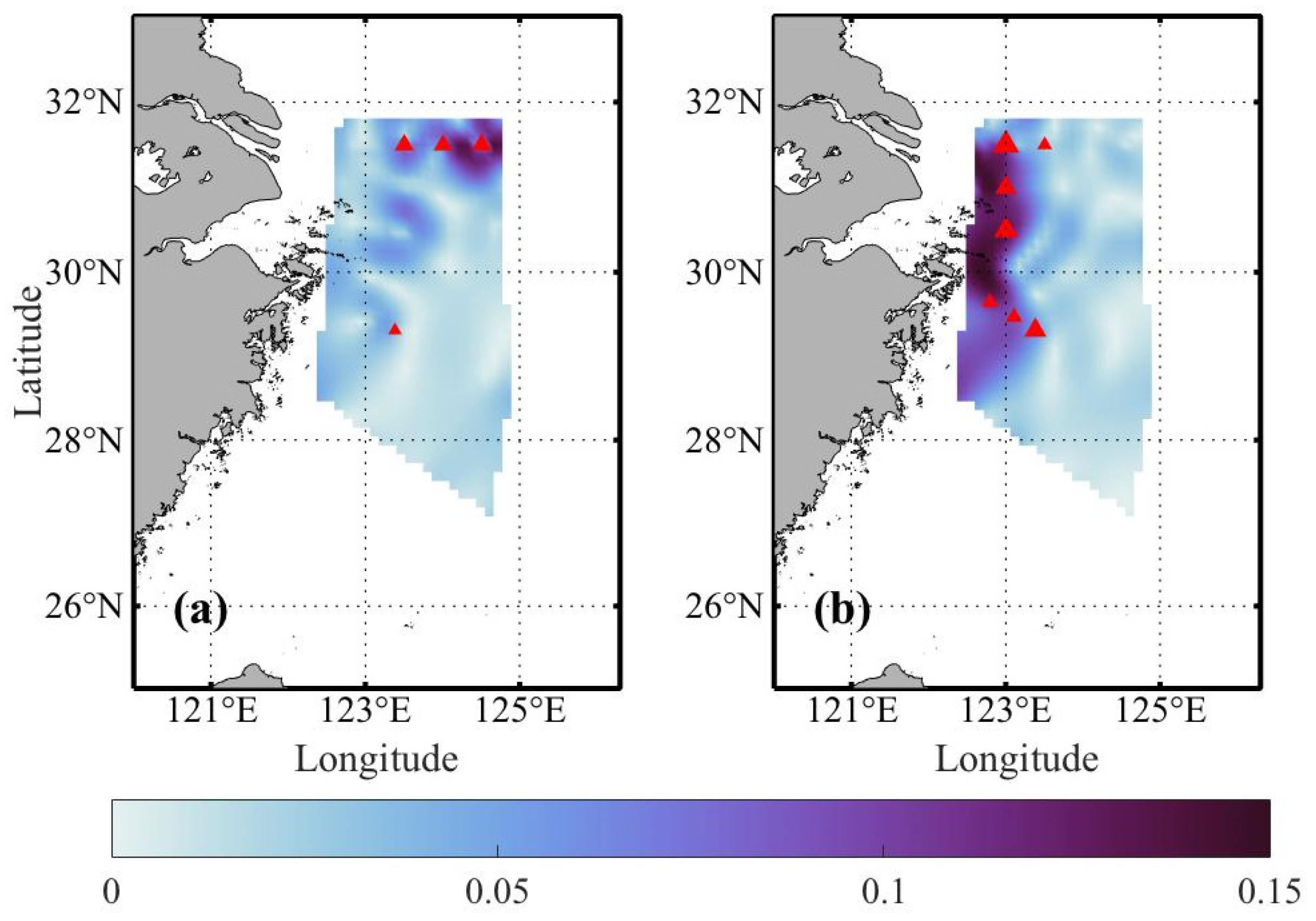
In order to explore the problem mentioned above, we use the interpolated results to present the spatial distribution of the gradient norm of the temperature and salinity. Take the cruise in summer 2010 as example. The gradient norm is calculated using the interpolation results of the 3D thin plate spline RBF method (Figure 7). Since the gradient is smaller at deeper layers, we choose the gradient at a −5 m depth for display. The MAEs are at the order of 10−2 in the 10-fold cross-validation experiments, and therefore, we present the locations of the observations where there is an absolute error larger than 10−1 (°C or psu) with the red triangles. The points in Figure 7a with a larger error are located in the northeast where the gradient norm of temperature is larger. While in Figure 7b, they are mainly located in the west side. The average gradient norms of the four cruises at a −5 m depth are shown in Table 5. The averaged gradient norm in summer 2010 for salinity is nearly twice as large as others, and the averaged gradient norms for temperature in summer 2010 and 2011 are larger than that in autumn as well. The size of the average gradient norms corresponds to the interpolation results well (Figure 3 and Figure 4). In addition, some boundary points are extrapolated. These two factors both contribute to the difference mentioned in the last paragraph.
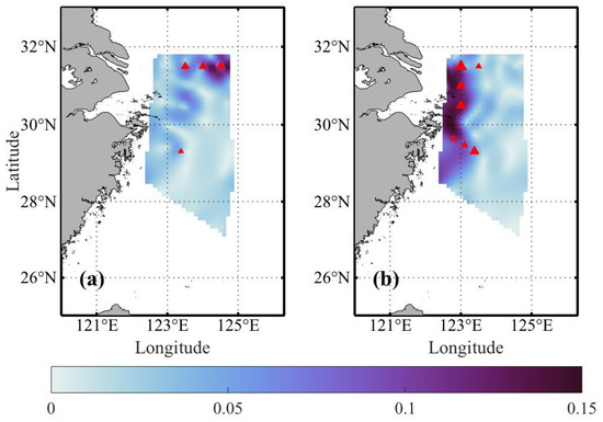
Figure 7.
Schematic diagram of the gradient norm distribution of the interpolation results with the thin plate spline RBF method at −5 m depth in summer 2010 (the unit are and for (a) and (b), respectively). The red triangles present the locations of the observations at −5 m depth where there is an absolute error larger than 0.1 (°C or psu) in the random 10-fold cross-validation experiments, and its size reflects the size of the error. (a) Temperature; (b) Salinity.

Table 5.
The average gradient norm at −5 m depth of four cruises.
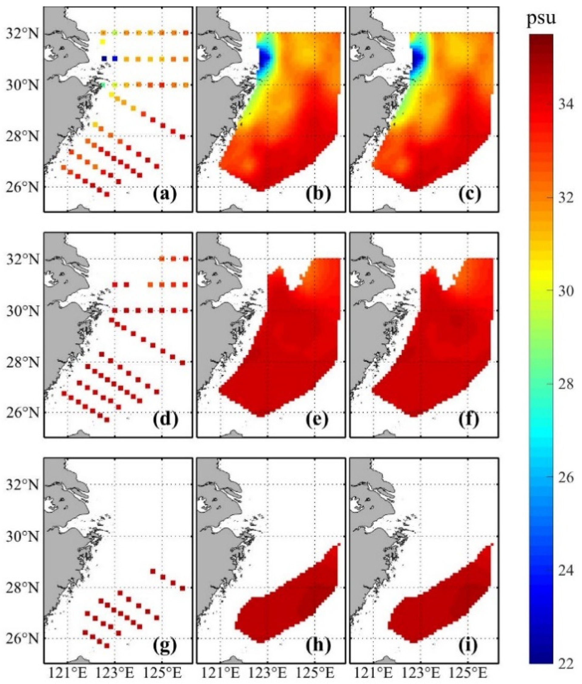
The thin plate spline and the cubic RBF method are similar as each as in MAEs. Therefore, we use the thin plate spline and the cubic RBF methods to reconstruct the 3D hydrologic structure in the ECS shelf for a comparison. Since data at numerous stations of the cruise in summer 2011 shows a larger discrepancy, we present its reconstructed results at several layers in Figure 8 and Figure 9. The results are similar, and they all largely coincide with the in situ observations. Therefore, in the circumstance of the hydrologic reconstruction in the ECS shelf, these two RBF methods are all recommended. Considering the good numerical stability and convergence of the thin plate spline RBF interpolation [33], the thin plate spline RBF reconstructions are chosen to present the results and explore the hydrologic variations in the ECS shelf.
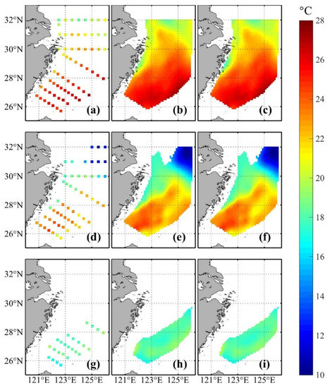
Figure 8.
The in situ temperature (summer 2011) and results reconstructed with different RBFs in the ECS shelf. The first column presents the in situ observations, the second is the interpolation result using the thin plate spline RBF method, and the last column uses the cubic RBF method. (a–c) −5 m depth; (d–f) −45 m depth; and (g–i) −85 m depth.
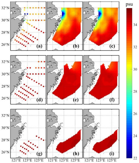
Figure 9.
The in situ salinity (summer 2011) and reconstructed results with different RBFs in the ECS shelf. The first column presents the original in situ observations, the second is the interpolation result using the thin plate spline RBF method, and the last column uses the cubic RBF method. (a–c) −5 m depth; (d–f) –45 m depth; and (g–i) −85 m depth.
3.4. The 2D RBF Method
The same 2D interpolation methods (IDW, CPF, and RBF methods) corresponding to the 3D interpolation introduced in the Section 3.1 and Section 3.2 methods were tested and we present the result using the thin plate spline RBF method with the data in summer 2011 for a test of the effectiveness of 2D interpolation. For the 2D method, the input vector is only a 2D horizontal vector and the vertical information is not included. The equation of the reconstructed field is changed and the input vector in Equations (5) and (6) is modified as a 2D vector. As for the Equation (1), it is changed correspondingly to Equation (10).
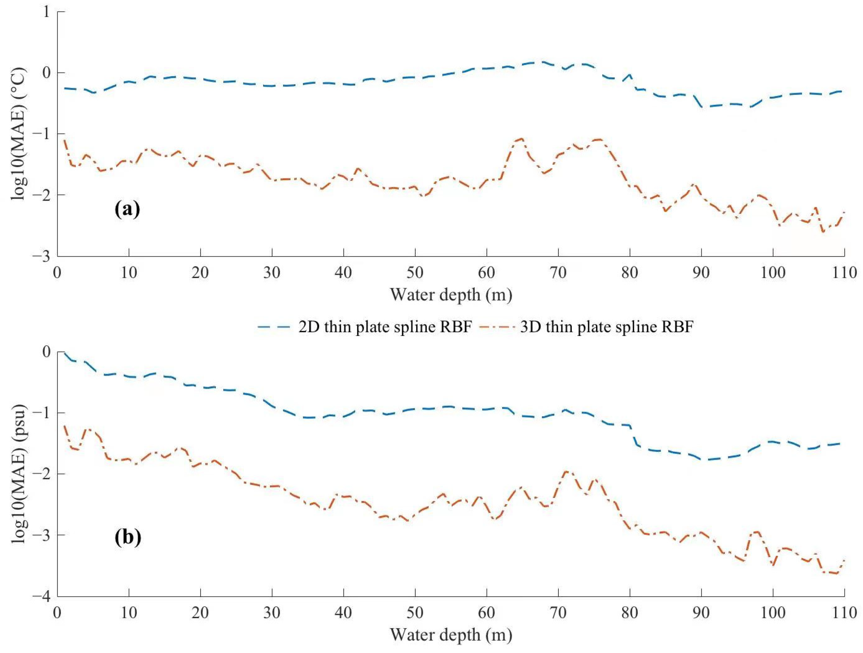
The average MAE of each depth is recorded in Figure 10. Compared with the 3D thin plate spline RBF method, the average MAE of the 2D method is obviously larger. Since observations at different depths show different patterns, the average MAE at each depth is different from each other. The average MAEs with the 3D thin plate spline RBF method at each depth are also computed. It shows an obvious advantage in the 3D reconstruction of the hydrologic factors in the ECS shelf. Other 2D methods (IDW and CPF) are also tested and the same conclusions are obtained (not shown). In conclusion, the 2D interpolation methods are not good at handling the 3D data because of insufficient data at the horizontal direction and its ignorance of the vertical information.
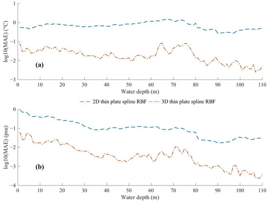
Figure 10.
The log10(MAE) at different depths with 2D and 3D thin plate spline RBF methods, respectively. The blue dash-dot line is the 2D thin plate spline RBF method while the orange dash-dot line is the 3D thin plate spline RBF method. (a) Temperature, (b) Salinity.
4. Application
4.1. Reconstruction and Water Mass Analysis
We reconstructed temperature and salinity at different depths which include −2 m, −5 m, −10 m, −20 m, −40 m, −60 m, −80 m, and −100 m. The boundary between coastal water mass and offshore water mass is obvious. In the southeast corner of the study area, with the increase in depth, the temperature decreases while the salinity increases.
The 3D reconstructed temperature (Figure 11a) and salinity (Figure 11b) in summer 2011 was shown for example. High temperature and low salinity water were observed in the upper layer (above −20 m) near the Yangtze River mouth. Because it is the flood time of the Yangtze River, warm and fresh water is diluted into the ECS and mixed with local ECS water. The results show that the influences of Yangtze diluted water decreased with depth and almost disappeared at −20 m. The cold area in the upper layer near the Zhejiang coast was induced by upwelling that brought the cold and saline water from a lower layer to the surface. High temperature and high salinity water can be resolved at the upper layer of the southeastern part of the ECS, which originated from Kuroshio in the ECS. With the increase in depth, the southeast of the ECS showed low temperature and high salinity that was attributed to the intrusion of the Kuroshio Branch Current to the northeast of Taiwan (KBCNT, [34,35]). The KBCNT originated from Kuroshio Subsurface Water with a temperature ranging from 13 to 25 ℃ and salinity ranging from 34.5 to 35.0 psu [7]. The low temperature water at the northeast of the ECS is considered to be the cyclonic eddy in the northern ECS [36], which is a subsurface cold eddy below −20 m with a low temperature. Overall, our method clearly resolves the water masses in the ECS.
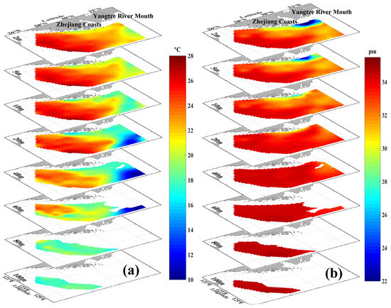
Figure 11.
The 3D reconstruction of the in situ observations in summer 2011. (a) Temperature; (b) Salinity.
To check the reconstruction results, we present T-S diagrams during the four cruises (Figure 12) to show various water masses. Similar to Figure 11, the T-S diagrams can clearly show the high salinity water from Kuroshio, which includes high temperature Kuroshio surface water and lower temperature Kuroshio subsurface water [7]. Coastal water in the north ECS including Yangtze River plume and Zhejiang upwelling water can also be identified in summer (Figure 12a,b). The coastal water cooling in autumn (Figure 12c,d) is significant compared with that in summer due to the air temperature falling and enhanced mixing driven by strong wind. The cold eddy in the north ECS is a phenomenon that can only be observed in summer and can be easily found in our reconstruction results.
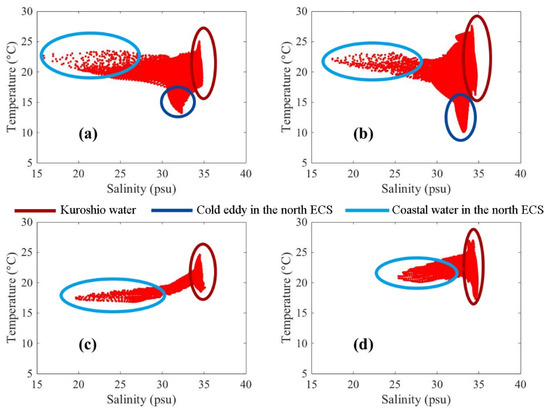
Figure 12.
The T-S diagram of interpolation results. (a) summer 2010; (b) summer 2011; (c) autumn 2010; and (d) autumn 2011.
An important current in the ECS is the intrusion of the KBCNT at the bottom layer, which can affect the water mass near the Yangtze River mouth and southwest of the Yellow Sea [1]. To check the RBF reconstruction results, we showed the distribution of bottom salinity in Figure 13, because the temperature is easily influenced by solar heating at the surface. In summer (Figure 13a), the east wind was prevailing near the Yangtze River mouth, which hindered the north intrusion of the KBCNT on the bottom because the east wind induces northward transport in the surface and thus the southward transport on the bottom. In summer (Figure 13b), the high salinity KBCNT was close to the Zhejiang coast, which may be due to the offshore Ekman transport on the surface by the south wind and onshore transport as a compensation. With the similar mechanisms to that in summer, the bottom KBCNT intrudes offshore in winter (Figure 13c,d). The high salinity tongue can intrude further north to the southwest of the Yellow Sea, because of the barotropic adjustment as described in [1]. Compared with the result in [8], using regular Cressman interpolation, this result can show more details of the intrusion process of the KBCNT and can help further explore the observation data.
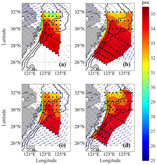
Figure 13.
The salinity distribution in the bottom layer. The black solid lines represent the −30 m, −50 m, and −70 m isobaths. The blue arrows are the wind field and the stations are depicted with the black triangles in the picture. (a) Summer 2010; (b) Summer 2011; (c) Autumn 2010; and (d) Autumn 2011.
4.2. Comparison with Satellite-Derived SST
The 3D RBF methods used in Section 3 perform better than the 2D RBF methods for the surface hydrologic conditions in the ECS shelf (Figure 10), which also shows a very small error in statistical analysis (the correlation coefficients in the 10-fold cross-validation experiments are larger than 0.99 and the MAEs maintain the order of ∼10−2). Considering the lack of in situ observations and the inaccuracy of the 2D interpolation methods, the 3D RBF reconstructions could reflect the SST more precisely and will not be disturbed by the spatial inconsistency. Therefore, the interpolated results are used to compare with satellite-derived SST and present the seasonal variability with analysis of influence factors.
Satellite-derived SST from MODIS could play an important role in the analysis of oceanic phenomena. The accuracy of the satellite was influenced by the platform, time, and the studied area. Previous studies show that the accuracy of MODIS-derived SST ranged from −0.06 °C to 0.8 °C and there was even a 2 °C bias in some areas [37,38]. The monthly MODIS-derived SST during daytime in summer and autumn 2010–2011 is used. As the in situ measurements have been interpolated onto the grids of satellite observations, there is no spatial mismatch between them. The interpolated results at −1 m depth are used to compare with the MODIS-derived SST.
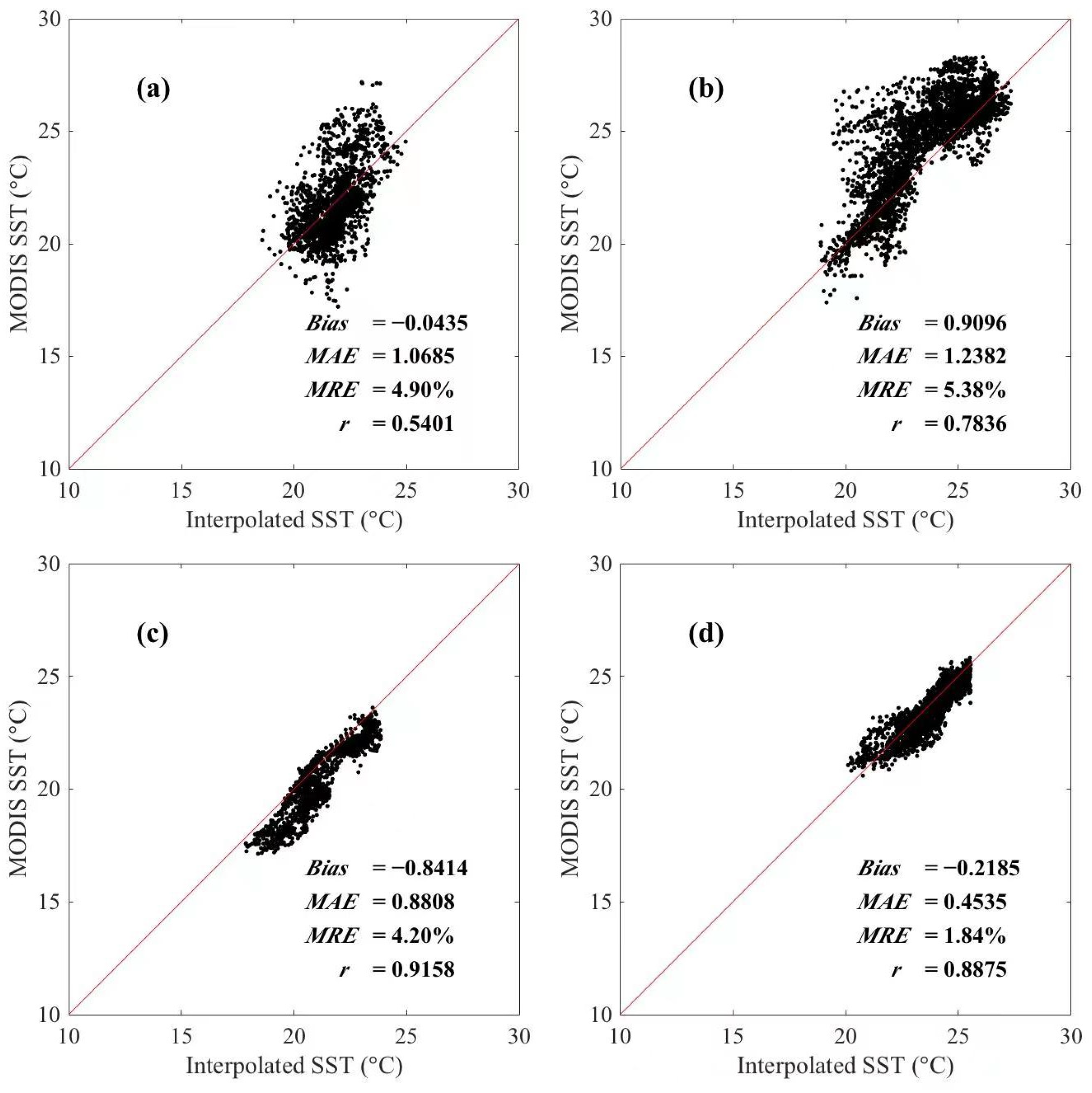
The standard deviation of MODIS-derived data has a seasonal variability. In summer it is in the range of 1.5 to 2.5 °C while in autumn it is in the range of 1 to 1.5 °C, indicating the seasonal variation of the SST in the ECS. The scatter plots presented in Figure 14 shows an obvious seasonal discrepancy. On the one hand, the MAE is 0.4535 °C in autumn 2011 and 0.8808 psu in autumn 2010. But it is larger than 1 °C in summer. Except the MAE, the MRE in summer is higher than that in autumn. Especially in autumn 2011, the MRE could reach the level of 1.84% while in other periods it is larger than 4%. Most points are located in the range of ±2 ℃ to the 1:1 line. At the same time, it can be seen from the scattered diagram that the distribution is more scattered in summer, presenting lower correlation coefficients, while it shows an obvious linear trend in autumn (Figure 14). On the other hand, the bias also presents seasonal variability. In summer 2011, the bias is positive while the bias is negative in autumn 2010 and 2011.
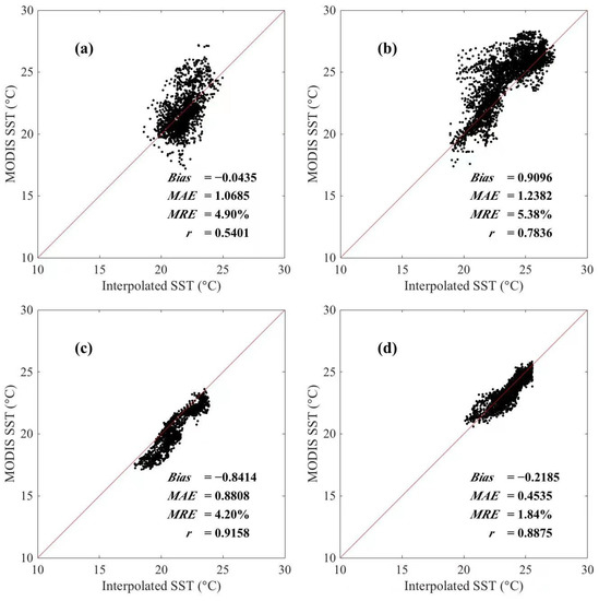
Figure 14.
Scattered plots of the match-up pairs between the interpolated SST and satellite-derived SST. (a) Summer 2010; (b) Summer 2011; (c) Autumn 2010; and (d) Autumn 2011.
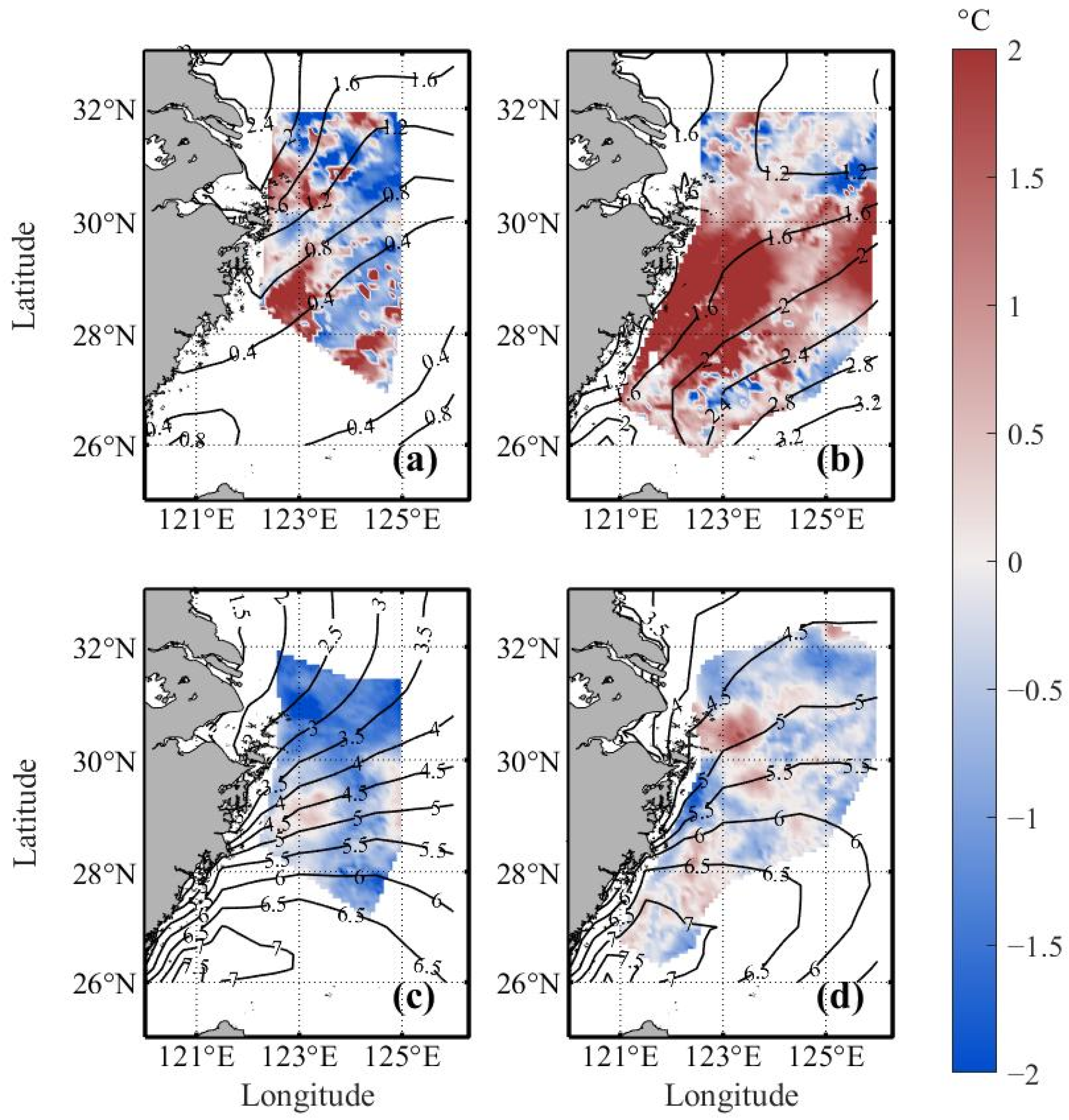
The possible causes of error are simply shown as follows. Firstly, the monthly MODIS SST was used, which introduced a possible large error in temporal consistency. Secondly, the obvious seasonal variability shown in the scatter plots is needed to be explored. Donlon et al. [39] carried out some tests to demonstrate that when the wind speed is greater than 2.5 m/s, the satellite-derived SST during the daytime and the nighttime will have a negative bias, while the wind speed is smaller than 2.5 m/s, the satellite-derived SST during the daytime will have a large positive bias. Therefore, we depict monthly wind speed contour maps and the bias distribution together in one picture (Figure 15). It can be seen that the wind speed in summer is significantly lower than that in autumn, and the wind speed in the area with a large error is largely below 2.5 m/s. The wind speeds in Figure 15c,d are largely higher than 2.5 m/s with small negative biases. At the same time, it can be seen in autumn 2010 that the area with a large error corresponds to the relatively smaller wind speed. The SST obtained from MODIS is the skin-SST while the ships measure the depth-SST. There is a discrepancy between them [40,41] which is possibly influenced by climate factors. Similar conclusions are mentioned in [42], which demonstrated that there would be a large positive bias between the skin-SST and depth-SST when the wind is weak during the daytime.
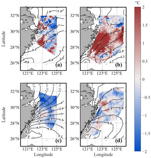
Figure 15.
The pictures of bias between the interpolated SST and the satellite derived SST together with the contour maps of the wind speed. (a) Summer 2010; (b) Summer 2011; (c) Autumn 2010; and (d) Autumn 2011.
Moreover, due to the large diurnal variability of SST in summer (long-time solar radiation), the error of the daytime data may be enlarged. Together with the small wind speed in summer, the vertical convective mixing is weak, which results in a shallow warm layer. The difference between the depth-SST and the skin-SST is greater than that in autumn when vertical mixing is stronger, which contributes to the large bias. At the same time, because of the impact of the fresh water of the Yangtze River in the summer, the hydrologic situation near the estuary is more complicated. Some fronts and vortices generated by the Kuroshio lead to a more complex temporal and spatial distribution of SST. These factors probably make more contribution to the lower correlation coefficients and larger errors in summer.
5. Summary
The 3D RBF interpolation schemes behave well for the data used in our paper. Based on sparse and unevenly distributed in situ observations, it could give complete reconstructed results with small errors. We tested other 3D interpolation methods and 2D methods to demonstrate the priority of the 3D RBF methods. Since the patterns of data play an essential part in choosing the RBFs, we also tested different 3D RBF methods. Our study shows the RBF method combined with the cubic or thin plate spline function is the optimal method for the reconstruction of temperature and salinity in the ECS shelf. Their MAEs could maintain the order of ~10−2 and the correlation coefficients between the observations and the interpolations are all larger than 0.99 in the 10-fold cross-validation experiments. In addition, the consistency of the change rate in different dimensions could contribute to the low MAEs. In fact, it is suggested that the horizontal and vertical change rates of target values in calculation are better to be adjusted to the same order of magnitude as far as possible, which may be beneficial to the small MAEs.
For the coherent 3D distributions of hydrological characters in the ECS, the 3D RBF interpolation could provide a more accurate result to explore the phenomena and related mechanisms. The 3D thin plate spline RBF interpolated results are presented not only for the 3D reconstruction but also for the satellite data evaluation. By comparing the interpolations and satellite-derived SST, we found that the large bias of satellite-derived data corresponds to weak mixing during weak wind. For the evaluation of the SST, the 3D RBF interpolation methods could give a more accurate result and could be applied in other regions with a lack of in situ observations.
Author Contributions
Conceptualization, X.L.; methodology, Y.G.; software, Y.G.; formal analysis, Y.G. and J.W.; investigation, Y.G.; writing—original draft preparation, Y.G.; writing—review and editing, J.W. and J.G.; supervision, X.L.; funding acquisition, X.L. All authors have read and agreed to the published version of the manuscript.
Funding
This work is supported by the Open Fund Project of Key Laboratory of Marine Environmental Information Technology, Ministry of Natural Resources of the People’s Republic of China, the National Natural Science Foundation of China (Grant Nos. 42076011, U1806214 and 41706012), and the Natural Science Foundation of Shandong Province of China (Grant No. ZR2020MD056).
Data Availability Statement
MODIS SST Level 3 product is produced by the NASA Goddard Space Flight Center’ s Ocean Data Processing System at https://oceancolor.gsfc.nasa.gov/, (accessed on 15 April 2022).
Acknowledgments
We would like to thank Zheng Guo and Shengyi Jiao for their friendly help. We deeply thank the reviewers and editor for their constructive suggestions on the earlier version of the manuscript.
Conflicts of Interest
The authors declare no conflict of interest.
References
- Weng, X.C.; Wang, C.M. A Preliminary Study on the T-S Characteristics and the Origin of Taiwan Warm Current Water in Summer. Stud. Mar. Sin. 1984, 21, 113–134. [Google Scholar]
- Guan, B.X. Major Features of the Shallow Water Hydrography in the East China Sea and Huanghai Sea. In Elsevier Oceanography Series; Elsevier: Amsterdam, The Netherlands, 1984; Volume 39, pp. 1–13. [Google Scholar] [CrossRef]
- Su, J.L.; Pan, Y.Q. On the Shelf Circulation North of Taiwan. Acta Oceanol. Sin. 1987, 6, 1–20. [Google Scholar]
- Zhou, F.; Xue, H.; Huang, D.; Xuan, J.; Ni, X.; Xiu, P.; Hao, Q. Cross-shelf exchange in the shelf of the East China Sea. J. Geophys. Res. Ocean. 2015, 120, 1545–1572. [Google Scholar] [CrossRef]
- Lie, H.J.; Cho, C.H.; Lee, J.H.; Lee, S. Structure and Eastward Extension of the Changjiang River Plume in the East China Sea. J. Geophys. Res. Ocean. 2003, 108, 1–14. [Google Scholar] [CrossRef]
- Ichikawa, H.; Chaen, M. Seasonal Variation of Heat and Freshwater Transports by the Kuroshio in the East China Sea. J. Mar. Syst. 2000, 24, 119–129. [Google Scholar] [CrossRef]
- Qi, J.; Yin, B.; Zhang, Q.; Yang, D.; Xu, Z. Analysis of Seasonal Variation of Water Masses in East China Sea. Chin. J. Oceanol. Limnol. 2014, 32, 958–971. [Google Scholar] [CrossRef]
- Wang, J.; Yu, F.; Ren, Q.; Si, G.; Wei, C. The Observed Variations of the North Intrusion of the Bottom Taiwan Warm Current Inshore Branch and Its Response to Wind. Reg. Stud. Mar. Sci. 2019, 30, 100690. [Google Scholar] [CrossRef]
- Qiu, B.; Toda, T.; Imasato, N. On Kuroshio Front Fluctuations in the East China Sea Using Satellite and in Situ Observational Data. J. Geophys. Res. Ocean. 1990, 95, 18191–18204. [Google Scholar] [CrossRef]
- Chang, Y.; Shimada, T.; Lee, M.A.; Lu, H.J.; Sakaida, F.; Kawamura, H. Wintertime Sea Surface Temperature Fronts in the Taiwan Strait. Geophys. Res. Lett. 2006, 33, 5–8. [Google Scholar] [CrossRef]
- Yin, W.; Huang, D. Short-Term Variations in the Surface Upwelling off Northeastern Taiwan Observed via Satellite Data. J. Geophys. Res. Ocean. 2019, 124, 939–954. [Google Scholar] [CrossRef]
- Mandal, S.; Behera, N.; Gangopadhyay, A.; Susanto, R.D.; Pandey, P.C. Evidence of a Chlorophyll “Tongue” in the Malacca Strait from Satellite Observations. J. Mar. Syst. 2021, 223, 103610. [Google Scholar] [CrossRef]
- Mandal, S.; Susanto, R.D.; Ramakrishnan, B. On Investigating the Dynamical Factors Modulating Surface Chlorophyll-a Variability along the South Java Coast. Remote Sens. 2022, 14, 1745. [Google Scholar] [CrossRef]
- Kilpatrick, T.; Xie, S.P.; Miller, A.J.; Schneider, N. Satellite Observations of Enhanced Chlorophyll Variability in the Southern California Bight. J. Geophys. Res. Ocean. 2018, 123, 7550–7563. [Google Scholar] [CrossRef]
- Siswanto, E.; Horii, T.; Iskandar, I.; Gaol, J.L.; Setiawan, R.Y.; Susanto, R.D. Impacts of Climate Changes on the Phytoplankton Biomass of the Indonesian Maritime Continent. J. Mar. Syst. 2020, 212, 103451. [Google Scholar] [CrossRef]
- Yu, Y.; Xing, X.; Liu, H.; Yuan, Y.; Wang, Y.; Chai, F. The Variability of Chlorophyll-a and Its Relationship with Dynamic Factors in the Basin of the South China Sea. J. Mar. Syst. 2019, 200, 103230. [Google Scholar] [CrossRef]
- Isa, N.S.; Akhir, M.F.; Kok, P.H.; Daud, N.R.; Khalil, I.; Roseli, N.H. Spatial and Temporal Variability of Sea Surface Temperature during El-Niño Southern Oscillation and Indian Ocean Dipole in the Strait of Malacca and Andaman Sea. Reg. Stud. Mar. Sci. 2020, 39, 101402. [Google Scholar] [CrossRef]
- Mandal, S.; Sil, S.; Shee, A.; Venkatesan, R. Upper Ocean and Subsurface Variability in the Bay of Bengal During Cyclone ROANU: A Synergistic View Using In Situ and Satellite Observations. Pure Appl. Geophys. 2018, 175, 4605–4624. [Google Scholar] [CrossRef]
- Urquhart, E.A.; Hoffman, M.J.; Murphy, R.R.; Zaitchik, B.F. Geospatial Interpolation of MODIS-Derived Salinity and Temperature in the Chesapeake Bay. Remote Sens. Environ. 2013, 135, 167–177. [Google Scholar] [CrossRef]
- Nie, Y.; Guo, J.; Sun, B.; Lv, X. An Evaluation of Apparent Color of Seawater Based on the In-Situ and Satellite-Derived Forel-Ule Color Scale. Estuar. Coast. Shelf Sci. 2020, 246, 107032. [Google Scholar] [CrossRef]
- Guo, J.; Nie, Y.; Li, S.; Lv, X. Application of Three-Dimensional Interpolation in Estimating Diapycnal Diffusivity in the South China Sea. J. Mar. Sci. Eng. 2020, 8, 832. [Google Scholar] [CrossRef]
- Hosoda, K.; Murakami, H.; Sakaida, F.; Kawamura, H. Algorithm and Validation of Sea Surface Temperature Observation Using MODIS Sensors Aboard Terra and Aqua in the Western North Pacific. J. Oceanogr. 2007, 63, 267–280. [Google Scholar] [CrossRef]
- Qin, H.; Chen, G.; Wang, W.; Wang, D.; Zeng, L. Validation and Application of MODIS-Derived SST in the South China Sea. Int. J. Remote Sens. 2014, 35, 4315–4328. [Google Scholar] [CrossRef]
- Ghanea, M.; Moradi, M.; Kabiri, K.; Mehdinia, A. Investigation and Validation of MODIS SST in the Northern Persian Gulf. Adv. Sp. Res. 2016, 57, 127–136. [Google Scholar] [CrossRef]
- Lam, N.S.N. Spatial Interpolation Methods: A Review. Am. Cartogr. 1983, 10, 129–150. [Google Scholar] [CrossRef]
- Li, B.; Liu, Y.; Wang, X.; Fu, Q.; Lv, X. Application of the Orthogonal Polynomial Fitting Method in Estimating Pm 2.5 Concentrations in Central and Southern Regions of China. Int. J. Environ. Res. Public Health 2019, 16, 1418. [Google Scholar] [CrossRef] [Green Version]
- Rocha, H.; Dias, J.M. Early Prediction of Durum Wheat Yield in Spain Using Radial Basis Functions Interpolation Models Based on Agroclimatic Data. Comput. Electron. Agric. 2019, 157, 427–435. [Google Scholar] [CrossRef]
- Geisser, S. The Predictive Sample Reuse Method with Applications. J. Am. Stat. Assoc. 1975, 70, 320–328. [Google Scholar] [CrossRef]
- Rocha, H. On the Selection of the Most Adequate Radial Basis Function. Appl. Math. Model. 2009, 33, 1573–1583. [Google Scholar] [CrossRef]
- Hubbert, S. Radial Basis Function Interpolation on a Sphere. Ph.D. Thesis, Imperial College London, London, UK, April 2002. [Google Scholar]
- Gutmann, H.M. A Radial Basis Function Method for Global Optimization. J. Glob. Optim. 2001, 19, 201–227. [Google Scholar] [CrossRef]
- Buhmann, M.D. Radial Basis Functions: Theory and Implementations, 1st ed.; Cambridge University Press: Cambridge, UK, 2003; pp. 4–5. [Google Scholar]
- Bartoli, A.; Perriollat, M.; Chambon, S. Generalized Thin-Plate Spline Warps. Int. J. Comput. Vis. 2010, 88, 85–110. [Google Scholar] [CrossRef]
- Yang, D.; Yin, B.; Liu, Z.; Feng, X. Numerical Study of the Ocean Circulation on the East China Sea Shelf and a Kuroshio Bottom Branch Northeast of Taiwan in Summer. J. Geophys. Res. Ocean. 2011, 116, 1–20. [Google Scholar] [CrossRef] [Green Version]
- Lian, E.; Yang, S.; Wu, H.; Yang, C.; Li, C.; Liu, J.T. Kuroshio Subsurface Water Feeds the Wintertime Taiwan Warm Current on the Inner East China Sea Shelf. J. Geophys. Res. Ocean. 2016, 121, 4790–4803. [Google Scholar] [CrossRef]
- Mao, H.L.; Hu, D.X.; Zhao, B.R.; Ding, Z.X. A cyclonic eddy in the northern East China Sea. In Proceedings of the International Symposium on Sedimentation on the Continental Shelf with Special Reference to the East China Sea, Hangzhou, China, 12–16 April 1983. [Google Scholar]
- Narayanan, M.; Thirumalai, D.; Bharadwaj, A.K.; Thanabalan, P.; Dhileeban, N. Comparison and Validation Of “Sea Surface Temperature (SST)” Using MODIS and AVHRR Sensor Data. Int. J. Remote Sens. Geosci. 2013, 2, 2319–3484. [Google Scholar]
- García, M.J.L. SST Comparison of AVHRR and MODIS Time Series in the Western Mediterranean Sea. Remote Sens. 2020, 12, 2241. [Google Scholar] [CrossRef]
- Donlon, C.J.; Minnett, P.J.; Gentemann, C.; Nightingale, T.J.; Barton, I.J.; Ward, B.; Murray, M.J. Toward Improved Validation of Satellite Sea Surface Skin Temperature Measurements for Climate Research. J. Clim. 2002, 15, 353–369. [Google Scholar] [CrossRef] [Green Version]
- Schluessel, P.; Emery, W.J.; Grassl, H.; Mammen, T. On the Bulk-Skin Temperature Difference and Its Impact on Satellite Remote Sensing of Sea Surface Temperature. J. Geophys. Res. 1990, 95, 13341–13356. [Google Scholar] [CrossRef]
- Kawai, Y.; Wada, A. Diurnal Sea Surface Temperature Variation and Its Impact on the Atmosphere and Ocean: A Review. J. Oceanogr. 2007, 63, 721–744. [Google Scholar] [CrossRef]
- Minnett, P.J.; Alvera-Azcárate, A.; Chin, T.M.; Corlett, G.K.; Gentemann, C.L.; Karagali, I.; Li, X.; Masouin, A.; Marullo, S.; Maturi, E. Half a Century of Satellite Remote Sensing of Sea Surface Temperature. Remote Sens. Environ. 2019, 233, 111366. [Google Scholar] [CrossRef]
Publisher’s Note: MDPI stays neutral with regard to jurisdictional claims in published maps and institutional affiliations. |
© 2022 by the authors. Licensee MDPI, Basel, Switzerland. This article is an open access article distributed under the terms and conditions of the Creative Commons Attribution (CC BY) license (https://creativecommons.org/licenses/by/4.0/).

