Article

Numerical Study of Circulation and Seasonal Variability in the Southwestern Yellow Sea

1
Key Laboratory of Marine Hazards Forecasting, Ministry of Natural Resources, Hohai University, Nanjing 210098, China
2
College of Oceanography, Hohai University, Nanjing 210098, China
3
Department of Oceanography, Dalhousie University, Halifax, NS B3H 4R2, Canada
*
Authors to whom correspondence should be addressed.
J. Mar. Sci. Eng. 2022, 10(7), 912; https://doi.org/10.3390/jmse10070912
Submission received: 19 May 2022 / Revised: 19 June 2022 / Accepted: 23 June 2022 / Published: 1 July 2022
(This article belongs to the Special Issue Numerical Modelling of Atmospheres and Oceans)

Abstract

:
A nested-grid ocean circulation modelling system (NGMS-swYS) is used for examining the impact of tides and winds on the three-dimensional (3D) circulation, hydrography and seasonal variability over the southwestern Yellow Sea (swYS). The modelling system is based on the Princeton Ocean Model (POM) and uses a nested-grid setup, with a fine-resolution (~2.7 km) inner model nested inside a coarse-resolution (~9.0 km) outer model. The domain of the outer model covers the China Seas and adjacent deep ocean waters. The domain of the fine-resolution inner model covers the swYS and adjacent waters. The NGMS-swYS is driven by a suite of external forcings, including the atmospheric forcing, tides, freshwater discharge and currents specified at the lateral open boundaries. A comparison of model results with observations and previous numerical studies demonstrates the satisfactory performance of the NGMS-swYS in simulating tides, seasonal mean circulation and distribution of temperature and salinity. Five additional numerical experiments were conducted using NGMS-swYS with different combinations of external forcing. Analysis of model results demonstrates that the monthly mean circulation over the swYS is affected significantly by tides and winds, with large seasonal variability. The northward Subei Shoal Current occurred in both winter and summer months in 2015, with persistent strong southeastward mean currents induced by tides along the 50 m isobath. Model results also demonstrated that strong wind-induced currents occurred with large sea surface cooling during Typhoon Chan-Hom.

1. Introduction

The southwestern Yellow Sea (swYS, see 
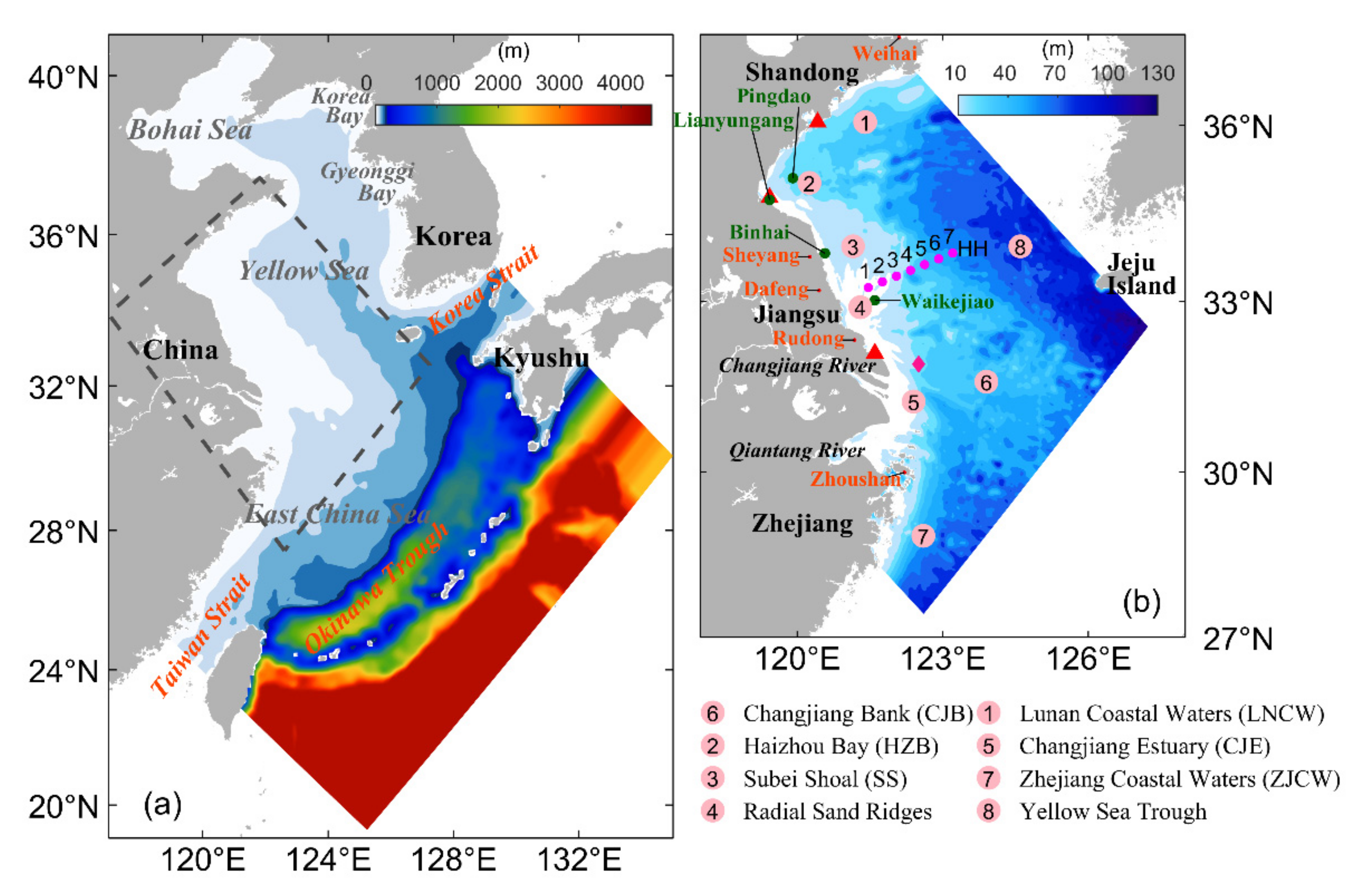
Appendix A for all abbreviations and symbols used in this paper) is a semi-enclosed marginal sea in the northwest Pacific Ocean, with an average water depth of about 44 m (Figure 1). The topography in the swYS is characterised by rugged coastlines and highly variable sea bottoms, with the Radial Sand Ridges (RSR) in the inner shelf region and the Yellow Sea Trough in the offshore region. Another important geographic feature in the swYS is the Changjiang Bank (CJB), which is a flat and broad shallow area located at the junction of the Yellow Sea and the East China Sea [1].
The hydrodynamics in the swYS was found to have significant seasonal variability [2,3,4]. The monthly mean oceanographic conditions in February and August are used in this paper to represent the winter and summer conditions. The February mean sea surface temperatures (SSTs) over the swYS (Figure 2a), inferred from the MURSST satellite remote sensing data over a 3-year period from 2014 to 16, vary from about 4 °C over the coastal waters off Shandong to about 14 °C in the deep waters around Jeju Island, with isotherms following approximately isobaths. The August mean SSTs during these 3 years are warm and in a range of 25–27 °C in the swYS (Figure 2b), with several patches of cold waters over the Subei Shoal (SS), HZB and Zhoushan Island [5,6]. The salinity over the swYS is affected by the spreading of low-salinity waters from the Changjiang (or Yangtze) River in both winter and summer months [7,8]. The Changjiang River is the largest river in China, which has an annual mean discharge of about 3.01 × 10 4   m 3 s−1, with significant seasonal and synoptic variability [9]. Over the swYS, the low-salinity (<31 psu) water in February is mainly confined to the Subei Shoal, Changjiang Estuary (CJE) and Zhejiang Coastal Water (ZJCW), with the 31 psu isohaline reaching 123°E to the east [8]. In August, with the increased Changjiang River discharge (CRD) and the intensified southerly monsoon, the Changjiang plume spreads mainly to the northeast and almost the entire swYS is covered with low-salinity waters. In comparison with the February condition, the freshwater tongue extending along the Zhejiang coast is greatly restricted in August [7].
The general circulation in the swYS includes the Yellow Sea Coastal Current (YSCC), Taiwan Warm Current (TWC), Yellow Sea Warm Current (YSWC) and Changjiang Plume (CJP). The circulation in the region is affected by the seasonally varying atmospheric forcing associated with monsoons [8,9,10,11], with the strong northeast monsoon in winter and the rain-bearing southwest monsoon in summer [4]. In winter, the shelf circulation system in the swYS normally features two major currents: a southeastward coastal current (known as the YSCC) flowing approximately along the 50 m isobath from the Lunan Coast Water (LNCW) to the CJB and a northwestward current (known as the YSWC). The latter separates from the Kuroshio Current and runs from the southwest of Jeju Island to the northern YS [10,11,12]. The circulation in the northern ECS features the weakly seaward CJP and northward TWC [9]. In summer, the YSCC in the swYS and the northward Korea Coastal Current (KCC) form the cyclonic circulation over the southern YS, while the YSWC disappears due to the adjustment of the circulation in the ECS. The CJP and TWC are enhanced in summer due mainly to the increase of the CRD and the effect of the southwest monsoon, respectively [13,14,15,16].
The general circulation and hydrography in the swYS (and also in the CJE) are significantly modulated by tides. The tidal residual currents were found to contribute more than 50% to the time–mean flow over the Changjiang Bank [1]. Over the RSR, the maximum tidal range reaches up to 9.4 m, and the tidal currents reach up to 2.5 m s−1 [17]. Over the SS, the tidally induced residual currents compensate for the wind-driven currents, leading to the counter-wind transport in winter months [1,8,13]. An upwelling branch over the swYS is caused by the large baroclinic gradient across the strong tidal mixing fronts (TMF), which is induced by tidal mixing over sloping topography in the swYS [18]. As a result, several cold water patches were observed in summer in this region [19].
The general circulation, hydrography and seasonal variability in the swYS were studied previously based on observations and numerical results [5,13,20,21,22,23,24,25]. The unfavourable natural and political conditions, however, have posed a great challenge to making successive and synchronous in situ observations over this region. With the advent of computer resources and advanced numerical methods, numerical ocean circulation models have increasingly been used in understanding the roles of tides and winds in the temporal and spatial variability of hydrography and circulation over the region. Naimie et al. [25] simulated the seasonal mean circulation in the YS and analyzed their dominant dynamics. Xia et al. [24] studied the three-dimensional (3D) structure of the summertime circulation of the Yellow Sea using the Princeton Ocean Model (POM). Wu et al. [26] examined the tidal effects on the CJP using the Estuarine, Coastal and Ocean Model (ECOM). Xuan et al. (2016) investigated the effect of tidal residual current on the mean flow over the CJB using the Finite Volume Coastal Ocean Model (FVCOM) [1]. Most of the previous studies focused on the hydrography and circulation in summer. Very limited studies, however, were made on wintertime hydrodynamics over the region. In this study, a nested-grid ocean circulation model was used to examine the impacts of tides and wind forcing on the hydrography, circulation and seasonal variability in the swYS. Our results will be useful in improving our knowledge of temporal and spatial variability of circulation and the main processes affecting the macroalgal blooms of Ulva prolifera in this region [27,28]. As suggested by Zhou et al. [20] and Wang et al. [21], the hydrographical structure, horizontal advection and vertical mixing play substantial roles in the phytoplankton bloom in the swYS.
This paper is arranged as follows. Observational and reanalysis data used in this study are introduced in Section 2. The nested-grid ocean circulation modelling system, external forcing and design of experiments are presented in Section 3. Assessment of the model performance is given in Section 4. The impacts of tides and winds on seasonal variations of hydrography and circulation are studied in Section 5. A conclusion is provided in Section 6.

2. Observational and Reanalysis Data

Four types of data are used in this study to drive the circulation model and to assess the model’s performance. These four types of data include satellite remote sensing data, in situ oceanographic observations, atmospheric reanalysis and hydrographic climatology. The satellite remote sensing data include the Multi-scale Ultra-high Resolution (MUR) SST data generated by the Jet Propulsion Laboratory of National Aeronautics and Space Administration [29]. The MURSST data are based upon the nighttime GHRSST L2P skin and subskin SST observations and in situ SST observations. The gridded MURSST data have a spatial resolution of 0.01° in longitude and latitude and at a daily frequency.
The in situ oceanographic data used to assess the model performance included the time series of sea surface temperature (SST) and sea surface salinity (SSS) observed at three stations (Figure 1b) over the Chinese coastal waters of the YS, namely the Xiaomaidao station (XMD), Lianyungang station (LYG) and Lvsi station (LVS). There were six hourly observations at 08:00, 14:00 and 20:00 (UTC + 8 h) at locations XMD and LYG and hourly observations at LVS in 2015. It should be noted that only the observed SSS at site XMD in 2015 were available for this study. These in situ data were provided by the National Marine Data Center (NMDC). The observed hourly surface elevations at Pingdao, Sheyang, Waikejiao and Lianyungang stations in July 2016 provided by the State Oceanic Administration were also used. The observed vertical profiles of temperature and salinity along transect HH (Figure 1b) were also used, which were conducted by Hohai University on 21 July 2016 using conductivity–temperature–depth (CTD) [5]. The observed vertical profiles of horizontal currents at station DD (its position is shown in Figure 1b) were also used, which were also conducted by Hohai University from 06:00 on 23 July to 08:00 on 24 July 2016 using the ADCP, with the sampling interval being 1 s. The ADCP data were averaged over 60 s time windows.
The monthly climatology of temperature and salinity digitised from the Marine Atlas of Bohai Sea, Yellow Sea and East China Sea (Hydrology) was also used to assess the model performance. This Marine Atlas was published by the Editorial Board for Marine Atlas based on the collection of historical observations between 1970 and 1992 [7].
The hourly CFSv2 atmospheric reanalysis data produced by the National Centers for Environmental Prediction (NCEP) of the United States [30] from 1 January 2014 to 31 December 2016 were used to force the ocean circulation model. The horizontal resolution of the CFSv2 data was ~0.2° × ~0.2°.

3. Nested-Grid Modelling System and Forcing

The ocean circulation model used in this study is the nested-grid modelling system for the southwestern Yellow Sea (hereafter NGMS-swYS) based on the POM [31]. The modelling system uses the nested-grid configuration similar to a triply-nested coastal circulation forecast system for the Pearl River Estuary developed by Sheng et al. [32]. The NGMS-swYS has two components (Figure 1): a coarse-resolution outer model and a fine-resolution inner model. The domain of the outer model covers the region between 117° E and 135° E and between 19° N and 41° N, including the Bohai Sea (BS), Yellow Sea (YS), East China Sea (ECS) and part of the Northwestern Pacific Ocean (NWPO), with a horizontal resolution about 9.0 km (Figure 1a). The 2-min Gridded Global Relief Data (ETOPO2) is used for the bathymetry in the outer model. The domain of the inner model covers the swYS and northern part of the ECS (Figure 1b), with a horizontal resolution of about 2.7 km. The 30 arcsec General Bathymetric Chart of the Oceans (GEBCO) bathymetry data are used in the inner model, except for the SS and CJE. Over areas of the SS and CJE, the fine-resolution topography in the model is based on the Marine Atlas published by the Ministry of Transport of the People’s Republic of China. Both the outer and inner models are 3D circulation models with 41 sigma levels for the vertical coordinates. The horizontal viscosity and diffusivity coefficients (Am and Ah) are calculated in the model using the scheme suggested by Smagorinsky [33], with the ratio of Ah to Am for the scheme being 0.1. The vertical viscosity and diffusivity coefficients Km and Kh are calculated using the modified Mellor-Yamada 2.5 turbulence closure scheme [34,35].
The initial conditions for temperature, salinity and velocity in the outer and inner models are taken from the daily mean products produced by an East Asian Marginal Seas model, with a horizontal resolution of 1/12° × 1/15° [36]. The external forcing for driving the outer and inner models of the NGMS-swYS in the control run (CR) includes the atmospheric forcing, tides, freshwater discharge and boundary forcing specified at the model lateral open boundaries. The atmospheric forcing includes the wind field taken from hourly NCEP atmospheric reanalysis. The bulk formula of Kondo [37] is used to convert the wind speed to wind stress. The net heat flux at the sea surface is calculated using shortwave radiation, long-wave radiation and sensible and latent heat fluxes in the model. All these components are calculated using the empirical formulas of Hirose et al. [38]. The net freshwater flux at the sea surface is calculated based on differences between precipitation and evaporation. The CRD is specified based on the monthly mean data published in the Chinese River Sediment Bulletin [39].
The tidal forcing at open boundaries of the outer model is specified using the radiation conditions for the depth-averaged currents and tidal surface elevations using the boundary condition suggested by Davies and Flather [40]. Four major tidal constituents (M2, S2, K1 and O1) are used based on the dataset produced by the TPXO ocean tidal circulation model [41]. The non-tidal components of the open boundary conditions are taken from the monthly mean reanalysis of the 1/2° × 1/2° surface elevations, currents, temperature and salinity produced by the Geophysical Fluid Dynamics Laboratory CM2.5 coupled circulation-ice model with a simple ocean data assimilation [42]. The GFDL CM2.5 coupled model has 1440 × 1070 eddy-permitting quasi-isotropic horizontal grid cells. The observed temperature and salinity assimilated into the GFDL CM2.5 model include the World Ocean Database of historical hydrographic profiles, in situ observations and satellite remotely sensed SST. More details of the model are reported by Carton et al. [42].
The surface elevations and depth–mean currents of tidal forcing at open boundaries of the inner model are specified using the same open boundary condition as in the outer model [40]. For the 3D currents, temperature and salinity, the adaptive open boundary condition is used at the open boundaries of the inner model based on the direction of currents (or waves) through the open boundary [43]. If the open boundary is active (i.e., outward propagations of waves through the open boundary), the state variables at the open boundary of the inner model are advected outward as freely as possible. If the open boundary is passive (i.e., inward propagations of waves through the open boundary), the state variables at the open boundary of the inner model are restored to the results produced by the outer model with a restoring time scale of one day.
Model results in five numerical experiments (Control Run, NoTide, NoWind, NT_CH, and NT_CH, see Table 1) are analyzed to examine the effects of tides and winds on seasonal variability in circulation and hydrography over the swYS. In the Control Run (CR), the NGMS-swYS is driven by the full suite of external forcing discussed above. In the case of NoTide (NT), the model setup and external forcing are the same in the CR, except for the exclusion of tidal forcing at the open boundaries of the outer model. In the case of NoWind (NW), the model setup and external forcing are the same in the CR, except that the wind forcing in the momentum equation and vertical turbulent kinetic energy equation is set to zero in the model. The NGMS-swYS in these three cases is integrated for three years from 1 January 2014 to 31 December 2016 (UTC). The model results of the last two years are used in this study. Two additional numerical experiments (cases NT_CH and NW_CH, Table 1) were conducted to examine the effects of tides and winds in circulation and hydrography over the swYS during Typhoon Chan-Hom. In the cases of NT_CH and NW_CH, the external forcing is the same in the CR, except for the exclusion of tidal forcing and wind forcing between 9 July and 12 July 2015. The model in cases NT_CH and NW_CH are integrated from 1 January to 31 December 2015.
For convenience, the swYS is divided into the coastal region with water depths shallower than 50 m and the offshore region with water depths deeper than 50 m. The coastal region includes the LNCW, SS, CJE and CJB. The offshore region consists of the YS Trough and adjacent deep water regions. Circulation and hydrography have significantly different features in these two regions.

4. Model Performance

We first assess the performance of the NGMS-swYS in simulating the tide elevations over the coastal and shelf regions of the NWPO. Figure 3 presents co-amplitudes and co-phases of M2, S2, K1 and O1 tidal elevations produced by the outer model of the NGMS-swYS in the case of CR. The simulated M2 tidal waves propagate into the ECS, the YS and the BS from the deep waters of the NWPO outside of the Ryukyu Islands (Figure 3a). The simulated M2 amplitudes increase from about 0.6 m in the deep ocean waters around the Ryukyu Islands to relatively large values over northern Taiwan Strait, Korea Strait and coastal waters off the western Korean Peninsula. The M2 amplitudes produced by the outer model are about 1.8 m over northern Taiwan Strait, 1.9 m in Korea Strait and greater than 2.2 m in Gyeonggi Bay. There are four M2 amphidromic points over the outer model domain, which are located in coastal waters off northwestern SS, Weihai of China and BS, respectively (Figure 3a). The general features of co-amplitudes and co-phases for M2 tidal elevations produced by the outer model agree with the previous model results made by Kang et al. [44], Guo and Yanagi [45] and Zhang and Sheng [46], and also tidal charts included in the Marine Atlas for the Bohai Sea, Yellow Sea and East China Sea [7].
The co-amplitudes and co-phases of M2 tidal elevations produced by the outer model in the case of CR (Figure 3a) are also compared to the counterparts from the TPXO ocean tidal model (Figure A1a in Appendix B). Both the outer model of the NGMS-swYS and the TPXO model generate very similar distributions of M2 tidal elevations, with differences in M2 amplitudes smaller than 0.1 m over most areas of the swYS. Over the northern Taiwan Strait and Korea Bay, however, the M2 amplitudes produced by the outer model in case CR are about 0.3 m smaller than the TPXO results, due most likely to the poor representation of the local bathymetry over these areas in the outer model. The locations of four M2 amphidromic points off northwestern Subei Shoal, Weihai of China and Bohai Sea produced by the outer model in case CR are consistent with the TPXO results (Appendix B).
The horizontal distribution of simulated S2 tidal waves is very similar to the M2 tidal waves, except for relatively smaller amplitudes of S2 tidal elevations than M2 tidal elevations. The simulated S2 amplitudes are about 0.5 m over coastal waters of southeastern China, about 0.2 m over the SS and larger than 0.6 m in Gyeonggi Bay. The simulated S2 tidal elevations also have four amphidromic points at locations very similar to the M2 tidal elevations. The general features of co-amplitudes and co-phases for S2 tidal elevations produced by the outer model agree very well with the previous model studies [7,45]. The S2 tidal wave propagations and locations of four amphidromic points produced by the outer model (Figure 3b) are also in very good agreement with the TPXO results (Figure A1b). The simulated S2 amplitudes produced by the outer model are slightly smaller than the TPXO results, with a maximum difference of about 0.2 m over Korea Bay.
The simulated K1 tidal waves produced by the outer model propagate northward from the deep ocean waters to the south of western Ryukyu Islands into the ECS, the YS and the BS (Figure 3c). The simulated K1 amplitudes are relatively large over the coastal waters of the western Korean Peninsula, with the largest amplitude of about 0.4 m over the coastal waters of Korea Bay. The K1 amplitudes are about 0.3 m and 0.1 m at the northern Taiwan Strait and SS, respectively. The simulated K1 tidal elevations have three amphidromic points located in the BS, the swYS and Korea Strait, respectively (Figure 3c). The general features of simulated K1 tidal elevations produced by the outer model agree well with the previous numerical results [44,45,46] and are also in good agreement with the TPXO results (Figure A1c in Appendix B). Some small differences occur over the Taiwan Strait and NWPO, where the simulated K1 amplitudes produced by the outer model are about 0.02 m smaller than the TPXO results.
Propagations of simulated O1 tidal waves produced by the outer model are very similar to the K1 tidal waves over the outer model domain, except for relatively smaller amplitudes for O1 tidal elevations than K1 tidal elevations. The simulated O1 amplitudes are about 0.3 m and 0.1 m over the coastal waters of Korea Bay and SS. The simulated O1 tidal elevations have two amphidromic points in the BS and the swYS, which are very similar to the locations of amphidromic points of K1 tidal elevations. The general features of simulated O1 tidal elevations produced by the outer model agree with the TPXO results (Figure A1d) and previous numerical studies [44,45,46].
We next assess the model performance by comparing the simulated surface elevations produced by the inner model in the case of CR (Figure 4) with the observations made at four tidal gauge stations of Pingdao, Sheyang, Waikejiao and Lianyungang in July 2016 (their positions are marked in Figure 1b). Three statistical metrics: Correlation coefficient (Corr), RMSE and γ 2 values [47] (Appendix C), are used to quantify the model performance. The correlation coefficients are about 0.98, 0.97, 0.95 and 0.98 at stations Pingdao, Sheyang, Waikejiao and Lianyungang, respectively. The RMSE values are about 0.22, 0.34, 0.48 and 0.36 m at these four stations, respectively. All these four RMSE values are smaller than 10 percent of the tidal range at these four stations, respectively. The γ 2 values are about 0.04, 0.16, 0.16 and 0.06 at these four stations, respectively. This indicates that the inner model of the NGMS-swYS has satisfactory skill in simulating surface elevations over the swYS.
We next examine the model performance in simulating the hydrography over the swYS. Figure 5 shows the monthly mean SSTs in February and August 2015 produced by the inner model in the case of CR (right panels) and derived from the satellite remote sensing data (left panels). In February (Figure 5b), the simulated monthly mean SSTs are cool and about 2 °C over the SS and LNCW; they are warm and about 16 °C or higher near the southwestern and southeastern areas of the inner model domain. The simulated February mean SSTs shown in Figure 5b indicate the influence of two warm currents, namely the TWC and the YSWC, which transport the high temperature (about 18 °C) and high salinity (about 34 psu) waters to the swYS in wintertime.
In August 2015, the surface water is significantly warmer than in February over the whole inner model domain (Figure 5d). The simulated August mean SSTs are about 26 °C over most areas of the swYS, except for a cold water patch of about 24 °C located off the SS [18]. This cold water patch indicates an upwelling off the SS in the summer months, as discussed in Lü et al. [18] and Wang et al. [23].
A comparison of the monthly mean SSTs produced by the inner model and satellite data (MURSST) demonstrates that the inner model reproduces well the SSTs over the inner model domain. The differences in the monthly mean SST between the inner model results and MURSST are less than 1.0 °C in both February and August over most areas of the swYS but relatively large and up to about 2.5 °C over the inner shelf of the SS in August (Figure 5c,d). The simulated August mean SSTs produced by the inner model (Figure 5d) are significantly warmer than the MURSST (Figure 5c) over the inner shelf due mainly to the fact of less reliable SSTs inferred from the satellite remote sensing data over coastal areas. In comparison, the simulated August mean SSTs produced by the inner model agree well with the previous numerical results produced by Huang et al. [19] over the inner shelf of the swYS. Furthermore, a comparison of the in situ hydrographic observations and simulated SSTs produced by the inner model at three Chinese coastal stations (to be shown later) also demonstrates that the NGMS-swYS reproduce well the SSTs over the inner shelf of the swYS.
Figure 6 presents the monthly mean sea bottom temperatures (SBT) in February and August produced by the inner model in the case of CR (right panels) and derived from the Marine Atlas for the Bohai Sea, Yellow Sea and East China Sea (Hydrology) [7] (left panels). In February, the distribution of the SBT produced by the inner model (Figure 6b) is very similar to the SST, as discussed above. This indicated that, in February 2015, the high-temperature TWC and YSWC flowed northward into the swYS in the whole water columns. The general features of the SBT produced by the inner model agree with the Marine Atlas (Figure 6a). However, the simulated SBT produced by the inner model implies that the TWC flows more northward to the eastern CJE and that the YSWC is weaker than the counterparts in the Marine Atlas.
In August 2015, the bottom layer of the YS Trough in the inner model was occupied by the relatively cool water lower than 8 °C (Figure 6d), known as the Yellow Sea Cold Water Mass (YSCWM) [48] extending from the central YS to the ECS. The August mean SBT produced by the inner model reaches up to 28 °C over the inner shelf, with sharp temperature gradients between the coastal warm water and YSCWM. The distribution of the simulated YSCWM in the YS Trough produced by the inner model agrees with the Marine Atlas (Figure 6c), except that the fringe of the YSCWM is significantly affected by the topography in the model results. Furthermore, the simulated SBT produced by the inner model is higher than the Marine Atlas over the coastal region.
The vertical distribution of observed temperature and salinity on 21 July 2016 along transect HH made by Hohai University is presented in Figure 7a,c. This transect extends from SS to YS Trough (marked in Figure 1b). Over the inner section of the transect (on the SS), the vertical stratification of observed temperature and salinity were vertically uniform and weakly stratified horizontally with vertically well-mixed temperature (salinity) varying from 26.2 °C (28.6 psu) at site HH1 near the coast to about 22.5 °C (31.3 psu) at site HH3. The observed low-salinity (<30 psu) water over the coastal area of transect HH (Figure 7c) originated from the CRD [13]. Over the central section of the transect, the vertical stratification of observed temperatures on 21 July 2016 was very strong in the top 15 m and vertically uniform below 20 m (Figure 7a). The observed salinity was vertically uniform in the top 10 m and below 20 m and slightly stratified vertically between 10 m and 20 m over the central section of transect HH (Figure 7c). Over the outer section of the transect close to the YS Trough, the observed temperature and salinity were nearly uniform vertically and horizontally and about 24.5 °C and 31.2 psu, respectively, in the upper mixed layer (at depths less than 10 m), with a strong thermohaline gradient at depths between 10 m and 20 m. Below 20 m, the observed hydrography over the outer section of the transect was vertically uniform and about 11.5 °C and 33.3 psu, respectively. The observed hydrographic profiles along transect HH (Figure 7a) also feature a well-defined upward climbing of bottom cold waters over the central section of the transect [19,23]. The observed temperature and salinity shown in Figure 7a,c represent the typical distribution of hydrography in the summer months over the swYS.
The simulated daily mean temperature and salinity on 21 July 2016 along transect HH produced by the inner model in the case of CR are compared with the hydrographic observations in Figure 7. The inner model reproduces very well the vertical distribution of observed temperature and salinity over the inner section of the transect (Figure 7b,d), with the simulated temperature (salinity) varying from 27.5 °C (29.2 psu) at HH1 to 23.2 °C (31.5 psu) at HH3 over the inner section of transect HH. The inner model also satisfactorily reproduces the observed upward climbing of bottom cold waters and the observed vertically uniform and horizontally stratified temperature and salinity below 20 m over the central section of the transect. Over the outer section of transect HH, the inner model reproduces reasonably well the uniform temperature and salinity in the surface layer of fewer than 5 m and the subsurface layer below 30 m. It should be noted that the thermocline in the model is too diffusive in comparison with observations, due mainly to a model deficiency [49].
Figure 8 presents the east-westward (U) and north-southward (V) currents at 5 m and 15 m depths at station DD derived from in situ observations (lines) on 23 and 24 July 2016. The CJB is dominated by strong reciprocating tidal currents, with the maximum current of about 1.89 m/s at 10:15 on 23 July. The maximum observed current occurs at the top layer of the water column. The observed currents decreased towards the bottom layer of the water columns. The simulated velocities produced by the inner model in the case of CR are in good agreement with the in situ observations horizontally and vertically. The RMSE values are about 0.09, 0.24, 0.07 and 0.19 m/s, and the γ 2 values are about 0.04, 0.09, 0.03 and 0.11 respectively for east-westward and north-southward velocities at 5 m and 15 m depths.
To assess the performance of the NGMS-swYS in simulating the seasonal cycle and synoptic variability of temperature and salinity, the simulated temperature and salinity produced by the inner model in the case of CR were compared with the hydrographic observations at three sites (XMD, LYG and LVS marked in Figure 1) over the Chinese coastal waters of western YS in 2015 provided by the NMDC (Figure 9). The observed SSTs at these three sites had large seasonal cycles, which increased from about 5 °C in the winter to about 30 °C in the summer in 2015 (Figure 9a,c,d). The observed SSTs at the three sites also had significant synoptic variability associated mainly with wind-driven upwelling and downwelling and other dynamic processes.
The simulated SSTs at three sites (XMD, LYG and LVS) produced by the inner model agree in general with the in situ observations, particularly the seasonal cycle (Figure 9a,c,d). It should be noted that the simulated SST at site XMD in the period between May and September 2015 was warmer than the observations, with differences reaching up to 3.5 °C on 6 August during Typhoon Soudelor. The RMSE and the γ 2 values are calculated using the time series of observed and simulated SSTs. The RMSE values are about 1.57 °C, 1.44 °C and 1.24 °C, and the γ 2 values are about 0.04, 0.03 and 0.02, respectively, for SSTs at sites XMD, LYG and LVS.
The observed SSS at site XMD does not have a large seasonal cycle but has significant synoptic variability (Figure 9b) associated mainly with wind-driven transport and precipitations. The observed SSS varied between 31.0 psu and 31.5 psu during the first six months of 2015 and decreased from 31.2 psu at day 197 to 29.7 psu at day 202 after Typhoon Chan-Hom on 12 July 2015 [50]. The observed SSS increased to 31.7 psu a few days after the storm. The inner model performs less well in simulating the SSS at site XMD (Figure 9b) with a relatively large γ 2 value of about 0.76, in comparison with the model performance in simulating the SST at the same site (Figure 9a). The RMSE value is about 0.42 psu for the SSS at site XMD. The main reason for the large model deficiency in simulating the SSS is that freshwater discharges from inlets along the Jiangsu coast are not included in the model simulation [51].

5. Physical Processes Affecting Seasonal Circulation and Hydrography

The three-dimensional (3D) circulation and hydrography in the swYS have significant seasonal variability, as shown above. The model results in 2015 in cases CR, NT and NW are examined in this section to investigate the main physical processes affecting the circulation and hydrography, with a special emphasis on the roles of wind and tidal forcing on the monthly mean fields.
We follow Wang et al. [52] and quantify the impacts of tides (and winds) on the seasonal circulation using the impact index ( P i ) defined as
P i = U C R U N T U C R + U N T
where U C R and U N T represent the monthly mean horizontal velocity vectors produced by the inner model in cases CR and NT, respectively, and A is the amplitude of the vector. It should be noted that ( U C R U N T ) includes the currents driven directly by tidal forcing and the nonlinear interactions of tidal currents with wind-driven currents and density-driven currents. The above-mentioned nonlinear interactions could not be produced by the circulation model with the tidal forcing only. The impact index for wind forcing can be calculated in the same way as in Equation (1) by replacing U N T with U N W .

5.1. Impacts of Tides and Winds on Seasonal Circulation

Figure 10a presents the February mean simulated currents in 2015 in the upper layer computed by vertically averaging the monthly mean currents produced by the inner model in the case of CR from the sea surface to 25 m. The monthly mean simulated circulation in the upper layer in this month features a strong northeastward jet (up to 0.17 m/s) known as the TWC, which flows from the southwestern area of the inner model domain (i.e., the inner shelf region off the Zhejiang coast) to the offshore waters. As reaching the southwestern flank of the CJB, this northeastward jet separates into two branches: an offshore branch turning anticyclonic and flowing southeastward to the south of the CJB, and an inshore branch flowing northward along the submarine canyon and then eastward to flow onto the central CJB (Figure 10a). The upper-layer simulated circulation in this month also has strong seaward currents (known as the CJP, up to 0.07 m/s) in the CJE and moderate seaward currents (up to 0.04 m/s) in the Qiantang Bay (QTB). A small branch of the seaward currents in the upper layer from both the CJE and QTB joins the inshore branch of the TWC to flow onto the central CJB, with most of the currents turning southwestward to form the Zhe-Min Coastal Current (ZMCC, up to 0.11 m/s). The February mean simulated Subei Coastal Currents (SCC, up to 0.06 m/s) over the SS flow northward along the Jiangsu coast, then turn southeastward at coastal water off Sheyang of China to flow offshore. The upper-layer simulated circulation in this month also features a strong southeastward circulation known as the YSCC (up to 0.11 m/s) over the southwestern YS Trough, which turns eastward at about 33.5°N to the north of Jeju Island (Figure 10a).
Figure 10d presents the February mean simulated currents in 2015 in the lower layer computed by vertically averaging the monthly mean currents produced by the inner model in the case of CR from the depth of 25 m to the sea bottom. The TWC also occurs in the lower layer in this month and flows northeastward from the southwestern corner of the inner model domain to the western CJB, with a maximum speed of about 0.18 m/s. A small offshore branch of the TWC turns anticyclonic to flow nearly eastward to the south of the CJB in the lower layer. The lower-layer circulation in this month has a weak cyclonic circulation (up to 0.03 m/s) over the central YS Trough (Figure 10d).
The effect of tidal forcing on the February mean circulation in terms of the tidal impact index (TII) is shown in Figure 10b for the upper layer and Figure 10e for the lower layer. In the upper layer, the effect of tidal forcing on the February mean circulation is significantly large, with the TII values greater than 0.6 over the inner shelf of the swYS, the YS Trough and the ZJCW. The tidal effect is also large for the February mean circulation in the upper layer, with the TII values between 0.2 and 0.6 over the eastern CJE. The TII values are relatively small for the main pathway of the TWC in the upper layer (Figure 10b).
The tidally induced monthly mean currents (TIMMCs, i.e., the monthly mean tidal residual currents) in the upper layer can be approximated by the differences ( Δ U U L t i d e ) in the monthly mean currents between cases CR and NT. The Δ U U L t i d e distribution in February 2015 (arrows in Figure 10b) was significantly affected by the complex topography in the swYS and reached up to about 0.03 m/s, 0.05 m/s and 0.07 m/s over the LNCW, SS and ZJCW, respectively. Over the YS Trough, the upper-layer TIMMCs in this month mainly flow southeastward along the 50 m isobaths, with a maximum value of about 0.12 m/s. Over the CJB, the Δ U U L t i d e distribution in this month shows several meso-scale tidal eddies (up to 0.10 m/s) flowing along the isobaths.
In the lower layer, the effect of tidal forcing on the February mean circulation is significantly large over the central YS Trough and eastern CJB, with the TII values greater than 0.6 (Figure 10e). The effect of tidal forcing on the TWC in the lower layer is relatively weak, which is similar to that in the upper layer. The TIMMCs in the lower layer in this month ( Δ U L L t i d e , arrows in Figure 10d) flow mainly along the YS Trough, with a maximum value of about 0.06 m/s. Similar to the Δ U U L t i d e over the CJB in this month, the lower-layer TIMMCs flow westward and turn southward to join the ZMCC, with a maximum value of about 0.05 m/s.
Figure 10c presents the effect of wind forcing on the February mean circulation in the upper layer (<25 m) in terms of the wind impact index (WII, image). In the upper layer, the effect of wind forcing on the February mean circulation is significantly large, with the WII values greater than 0.6 over the LNCW, the northwestern YS Trough and the southeast part of the inner model domain. Over other areas, the wind effects in the upper layer are relatively weak for the February mean circulation, with the WII values smaller than 0.4.
The wind-induced monthly mean currents (WIMMCs) in the upper layer are represented by the velocity differences ( Δ U U L w i n d ) in the monthly mean currents between cases CR and NW. The Δ U U L w i n d values in February 2015 (arrows in Figure 10c) are very weak over the HZB, SS and CJE. The northward WIMMCs (about 0.05 m/s) in the upper layer flow along the YS Trough from the southwest of Jeju Island to the central YS.
The effect of wind forcing on the February mean currents in the lower layer (>25 m) is shown in Figure 10f in terms of the WII (image). The wind effect is significantly large for the February mean circulation in the lower layer, with the WII values greater than 0.6 over the northwestern YS Trough and relatively weak over other areas. The lower-layer WIMMCs are represented by the velocity differences ( Δ U L L w i n d , arrows in Figure 10f) in this month between cases CR and NW. The lower-layer WIMMCs in this month flow northward along the YS Trough (up to 0.05 m/s) and are very weak over other areas.
Figure 11a presents the simulated August mean currents in 2015 in the upper layer (<25 m) computed using the same method as in Figure 10a. In the upper layer, the pathway of the TWC is very similar in February and August, except that it is stronger in August (up to 0.5 m/s) than in February. In the upper layer, the monthly mean CJP is significantly stronger in August (up to 0.12 m/s) than in February 2015 since the CRD is significantly larger in summer months than in winter months. Most of the CJP turns northeastward to flow onto the swYS after leaving the CJE. The monthly mean northward SCC in the upper layer also becomes stronger in August (up to 0.08 m/s) than in February 2015 over the SS. Over the YS Trough, the upper layer circulation in August features a strong cyclonic circulation, with a strong southeastward circulation (up to 0.3 m/s) flowing along the 50 m isobath and turning eastward at about 33°N to the northwest of the Jeju Island.
Figure 11d presents the August mean simulated currents in the lower layer (>25 m) computed using the same method as in Figure 10d. In comparison with the counterpart in February, the TWC in the lower layer is relatively stronger in this month, with a maximum speed of about 0.2 m/s. Most of the TWC in the lower layer flows northward along the submarine canyon to the CJB. The lower layer circulation in this month also has a weak cyclonic circulation (up to 0.05 m/s) over the central YS Trough.
The effect of tidal forcing on the August mean circulation in terms of the TII is shown in Figure 11b for the upper layer and in Figure 11e for the lower layer. In the upper layer, the effect of tidal forcing on the August mean circulation is significantly large, with the TII values greater than 0.6 over the northern and western YS Trough, the CJE, the QTB and the ZJCW. The tidal effect is also large for the August mean circulation in the upper layer, with the TII values between 0.2 and 0.6 over the HZB and the inner shelf of the SS. TII values are relatively small for the central CJB and the pathway of the TWC.
The strong TIMMCs in the upper layer in August ( Δ U U L t i d e , arrows in Figure 11b) are cyclonic and run along approximately the 50 m isobaths over the YS Trough and feature a southwestward flow over the ZJCW from the CJE to the southwestern of the model domain. The Δ U U L t i d e values in this month reach up to about 0.3 m/s, 0.3 m/s and 0.2 m/s over the northern and western YS Trough and the ZJCW.
In the lower layer, the effect of tidal forcing on the August mean circulation is significantly large, with the TII values greater than 0.6 over the LNCW and the YS Trough (Figure 11e). Over other areas, the tidal effect for the August mean circulation in the lower layer is relatively weak. The Δ U L L t i d e distribution in August (arrows in Figure 11e) demonstrates that the lower-layer TIMMCs mainly move along the YS Trough (up to 0.18 m/s) and have a mesoscale eddy (up to 0.07 m/s) off the CJE in the lower layer.
The TIMMCs in August have flow directions similar to the February condition in both upper and lower layers. However, the magnitudes of the southeastward TIMMCs along the western slope of the YS Trough in August are larger than that in February in both upper and lower layers, due to the interaction between tidal currents and baroclinicity, since the temperature and salinity are highly-stratified in summer months in the swYS.
Figure 11c presents the effect of wind forcing on the August mean currents in the upper layer (<25 m) in terms of the WII (image). In the upper layer, the effect of wind forcing on the August mean circulation is significantly large, with the WII values greater than 0.6 over the LNCW, the main pathway of TWC and the southwest area of Jeju Island. The wind effect is also large for the August mean circulation, with the WII values between 0.2 and 0.6 over most areas of the SS. The WII values are relatively small in this month over the main pathway of the YSCC and eastern CJB. The Δ U U L w i n d distribution (arrows in Figure 11c) in August demonstrates that the upper-layer WIMMCs are strong, with maximum values respectively reaching up to about 0.31 m/s, 0.08 m/s, 0.05 m/s and 0.22 m/s over the ZJCW, the CJB, the LNCW and the west area of Jeju Island. In the upper layer, the WIMMCs flow northward over the ZJCW, the CJE, the SS and the LNCW to the northern YS. The upper-layer WIMMCs in this month feature an anticyclonic circulation over the northwest Jeju Island and a cyclonic circulation over the southwest Jeju Island.
The effect of wind forcing on the August mean currents in the lower layer (>25 m) is shown in Figure 11f in terms of the WII (image). In the lower layer, the wind effect is significantly large for the circulation in this month, with the WII values greater than 0.6 over the west areas of Jeju Island. The effect of wind forcing on the August mean circulation is large, with the WII values between 0.2 and 0.6 over the western areas of the model domain. WII values are relatively small for the central YS Trough and eastern CJB in the lower layer. The Δ U L L w i n d distribution in this month (arrows in Figure 11f) features a northeastward WIMMCs over the ZJCW (up to 0.11 m/s) and a southward WIMMCs over the west area of Jeju Island (up to 0.07 m/s). The WIMMCs are relatively weak in the lower layer over other areas.
The above analyses demonstrate that, in February 2015, the WIMMCs flow against the northward SCC over the SS, and the northward YSWC along the YS Trough in the lower layer was enhanced by the wind-induced barotropic pressure gradient. By comparison, in August 2015, the southwesterly summer monsoon was generally weak and had minor impacts on the circulation in the lower layer. The TIMMCs were the dominant currents over the coastal region of the swYS and YS Trough in both February and August 2015.

5.2. Impacts of Tides and Winds on Seasonal Hydrography

The differences in the monthly mean SST ( Δ T S t i d e ) and SSS Δ S S t i d e between cases CR and NT were used to quantify the effects of tidal mixing and advection on the monthly mean hydrography over the swYS. In February 2015, the Δ T S t i d e values (Figure 12a) were relatively large and up to 2.2 °C over the deep waters off the SS and along the 50 m isobaths, due mainly to the transport of cold water by the TIMMCs from the northern YS to the swYS. In comparison, the Δ T S t i d e values are very small over the SS in this month. The Δ S S t i d e values in this month (Figure 12c) are significantly negative over the CJE and the coastal water off Sheyang of China, with maximum negative values of about −7.8 psu over the CJE and about −6.5 psu over the coastal water off Sheyang of China, which are mainly due to the effect of the unique tidal wave system over the swYS [8], which means that the northward TIMMCs from the CJE and the southward TIMMCs from the LNCW merge over the coastal water off Sheyang of China, then turn eastward to flow offshore, and the TIMMCs over the RSR spread seaward [51]. The tidal residual currents transport high salinity water from the offshore area to the RSR; thus, positive Δ S S t i d e values (up to 6.5 psu) occur in this region.
The differences ( Δ T S w i n d ,   Δ S S w i n d ) in the monthly mean SST and SSS between cases CR and NW are used to quantify the effect of wind forcing on the monthly mean hydrography at the sea surface. It should be noted that the simulated SSTs in the case of NW have similar seasonal cycles as the counterparts in the case of CR since wind forcing is used in calculating the net surface heat flux in case NW. If the wind forcing is set to zero in the calculation of the net surface heat flux, the model does not generate the seasonal cycles in the SST. Therefore, only the role of advection and vertical mixing generated by wind forcing on the hydrographic distribution over the swYS is considered based on differences in simulated hydrography between cases CR and NW.
The Δ T S w i n d values in February 2015 (Figure 12b) are negative and up to −3.0 °C over the CJB, due mainly to the advection of cold water from the northern YS to the CJB by WIMMCs. The Δ T S w i n d values are positive and up to 2.8 °C over the main pathway of the TWC in this month, due mainly to the wind-induced vertical mixing between the cool surface water and warm TWC water. The Δ S S w i n d values in this month (Figure 12d) are positive and up to 6.5 psu over the CJE and the coastal water off Rudong of China and positive and up to 4.8 psu over the coastal water off Sheyang of China. The Δ S S w i n d values in this month are negative and up to −2.0 psu over the coastal water off Dafeng of China. The northerly winter monsoon blocks the northward transport of the CRD induced by TIMMCs; thus, the distribution and values of Δ S S w i n d are opposite with the Δ S S t i d e (Figure 12c,d).
Similarly, the differences ( Δ T B t i d e ,   Δ S B t i d e ) in the monthly mean SBT and SBS between cases CR and NT are used to quantify the effect of tidal forcing on the monthly mean hydrography at the sea bottom. The Δ T B t i d e values in February (Figure 13a) are negative and up to −3.0 °C over the western of CJB in this month, due mainly to the strong tidal mixing. Similar to the Δ T S t i d e , the Δ T B t i d e are negative and up to −2.0 °C over the deep water along the 50 m isobaths due to the transport of cold water from northern YS to the swYS by southeastward TIMMCs along the western slope of the YS Trough. The distribution of Δ S B t i d e in this month (Figure 13c) is very similar to Δ S S t i d e , with the Δ S B t i d e being negative and up to −8.2 psu over the CJE, negative and up to −5.3 psu over the coastal water off Sheyang of China and positive and up to 6.5 psu over the RSR. The dynamical factors for the specific distribution of Δ S B t i d e are the same as Δ S S t i d e , as discussed above.
Figure 13b,d presents differences ( Δ T B w i n d ,   Δ S B w i n d ) in the February mean SBT and SBS between cases CR and NW. The large Δ T B w i n d are negative and up to −3.5 °C over the CJB and the submarine canyon off the CJE (Figure 11b), due to the advection of cold water from northern YS to this region by WIMMCs and wind-induced mixing. The distribution of Δ S B w i n d in this month is similar to Δ S S w i n d over the SS, with positive values (up to 6.5 psu) over the coastal water off Rudong, positive values (up to 4.2 psu) over the coastal water off Sheyang and negative values (up to −2.0 psu) over the coastal water off Dafeng. The monthly mean SBS is weakly decreased (by up to 1.5 psu) over the main pathway of the TWC in this month due to the wind mixing between the subsurface high-salinity TWC water and surface low-salinity CRD.
In August 2015, the Δ T S t i d e values (Figure 14a) are positive and up to 3.0 °C over the shallow side of 30 m isobaths due to the transport of coastal warm water by the TIMMCs. The strong tidal mixing over the deep side of 30 m isobaths plays an important role in reducing the SST in this month. Over the western slope of the YS Trough, the southeastward TIMMCs transport cold and high-salinity water from the northern YS to the swYS. As a result, the Δ T S t i d e values are negative (up to −1.8 °C) and the Δ S S t i d e values (Figure 14c) are positive (up to 5.0 psu) over the northern part of the swYS and the western slope of the YS Trough in this month. The Δ S S t i d e values in the same month are negative and up to −9.8 psu over the inner shelf of the SS and the QTB due to the tidal transport of the CRD.
Distribution of negative values of Δ T S w i n d in August (Figure 14b) demonstrates that the monthly mean SSTs are reduced by wind-induced vertical mixing over the entire swYS, except for the HZB and SS since the water temperatures are relatively warm and uniform over these regions. The large and negative values of Δ T S w i n d over the LNCW (up to −1.0 °C), ZJCW (up to −3.0 °C) and waters off the SS (up to −2.3 °C) are associated with the wind-driven upwelling [6,10]. The Δ S S w i n d values in this month (Figure 14d) are negative (up to −9.0 psu) over the northern and eastern part of the inner model domain and positive (up to 8.6 psu) over the CJE and ZJCW since the southwesterly winds block the southward transport of the CJP and push the CJP to extend northward.
Figure 15 presents the effects of tides and winds on the August mean SBT and SBS. The Δ T B t i d e values in this month (Figure 15a) are positive and up to 7.2 °C over the CJB, and up to 4.5 °C over the LNCW, the HZB and the ZJCW. The positive Δ T B t i d e over the CJB are mainly due to the strong tidal mixing. Over the shallow side of the 30 m isobaths in this month, the Δ T B t i d e values are positive and highly similar to the positive Δ T S t i d e values, which are generated by the tidal transport of warm coastal water. Very similar to the Δ S S t i d e values, the Δ S B t i d e values in August 2015 (Figure 15c) are negative and up to −10.0 psu over the CJE and the QTB and positive (up to 3.5 psu) over the north of the model domain. The dynamical factors for the distribution of Δ S B t i d e are the same as Δ S S t i d e in this month, as discussed above. The Δ S B t i d e values in this month are very small over the central YS Trough due to the blocking effects of the strong TMF in summer months.
The Δ T B w i n d values in August (Figure 15b) are positive and up to 5.2 °C over the CJB, and up to 5.0 °C over the southern LNCW, due mainly to the advection of warm water from the southern part of the inner model domain by WIMMCs and wind-induced vertical mixing. The southwesterly summer monsoon contributes to the northward transport of the CRD and depresses the southward moving of the CRD; as a result, the Δ S B w i n d values are negative and up to −9.5 psu over the inner shelf of the SS, and positive and up to 7.2 psu over the QTB and inner shelf of the ZJCW in this month (Figure 15d).
Based on differences in SST, SBT, SSS and SBS between cases CR and NT in February and August 2015, tidal residual currents are found to play an important role in the northward movement of the CRD over the coastal region and southeastward movement of waters from northern YS to the swYS, which have significant effects on the water exchange between different regions in both seasons. The strong tidal stirring also enhances the mixing of the surface and subsurface waters over the regions between 30 m and 50 m isobaths in February and August. The northerly winter monsoon transports cold water from the northern YS to the swYS and blocks the northward advection of CRD, while the upwelling-favourable southwesterly wind in summer enhances the northward advection of CRD and inshore transport of bottom waters in the swYS. The wind-induced mixing also contributes to the exchange of surface and subsurface waters in both seasons.
We next examine the effects of tides and winds on the vertical distribution of monthly mean temperature and salinity along transect HP (shown in Figure 5a) based on the inner model results in the case of CR. In February 2015 (Figure 16a,b), the vertically uniform cold (about 5.7 °C) and low-salinity (about 29.3 psu) waters occurred in the inner section of transect HP, while vertically uniform warm (about 9.3 °C) and high salinity (about 34.1 psu) water covered the YS trough of transect HP.
The differences in the February mean temperature and salinity between CR and NT ( Δ T H P t i d e ,   Δ S H P t i d e ) along transect HP are presented in Figure 16c,d. Over the inner section of transect HP in this month, the Δ S H P t i d e values are vertically uniform and vary in the offshore direction from positive values (up to 4.0 psu) over the western inner section of transect HP to negative values (up to −2.0 psu) over the eastern inner section (Figure 16d), due mainly to the northward transport of the CRD under the unique wave system mentioned earlier. By comparison, the Δ T H P t i d e values are near zero (<0.4 °C) over the inner section of transect HP in the same month (Figure 16c) since the water temperatures are relatively cool (about 5.7 °C) and nearly uniform vertically and horizontally over the inner shelf of the SS in winter months. These relatively cool waters over the inner shelf in winter months are generated by winter convection. Over the central section of transect HP, the Δ T H P t i d e values are relatively large and negative (up to −2.0 °C) and the Δ S H P t i d e values are vertically uniform and vary from about −1.2 psu on the west side to 1.5 psu on the east side (Figure 16c,d), due mainly to the TIMMCs over the SS. Over the outer section of transect HP, the Δ T H P t i d e values are negative (up to −1.2 °C) and Δ S H P t i d e values are relatively small and positive (up to 1.5 psu) due to the tide-induced transport of high salinity water from northern YS to the central swYS.
The differences in the February mean temperature and salinity between CR and NW ( Δ T H P w i n d ,   Δ S H P w i n d ) along transect HP are presented in Figure 16e,f. Over the inner section of the transect, the Δ T H P w i n d values in this month are also small and less than 0.4 °C (Figure 16e), due mainly to the uniform temperatures vertically and horizontally over the inner shelf of the SS in this month. It should be noted that wind forcing plays a very important role in the net heat flux at the sea surface, as mentioned earlier. The Δ S H P w i n d values in this month are vertically uniform and vary from a positive value of about 1.5 psu near the coast to negative values of about −1.3 psu over the offshore waters over the inner section of the transect (Figure 16f) due to the transport of the CRD generated by wind forcing. Over the central section of transect HP in this month, the Δ T H P w i n d values are nearly vertically uniform varying from about −1.2 °C on the west side to about 1.0 °C on the east side (Figure 16e), and the Δ S H P w i n d are positive and up to 1.2 psu at the east side of this section (Figure 16f), due mainly to the wind-induced transport of cold and high salinity water from the northern YS. The Δ T H P w i n d values in this month are positive and up to 1.2 °C in the top 10 m at about 122.7°E over the outer section due to the wind-induced transport of warm waters from the southwest of Jeju Island (Figure 16e). The Δ S H P w i n d are negative and very small (up to −0.5 psu) over the outer section of transect HP in this month, due mainly to the transport of CRD and wind-induced vertical mixing.
The vertical distribution of the August mean temperature and salinity produced by the inner model in case CR is presented in Figure 17a,b. The monthly mean temperature and salinity in this month are vertically uniform and weakly stratified horizontally over the inner section of transect HP. The vertically well-mixed temperature and salinity in this month vary from 28.2 °C and 27.7 psu over the western side near the coast to about 26.5 °C and 32.6 psu over the eastern side of the inner section. Over the central section of transect HP, the vertical stratification of the August mean temperature is strong in the top 15 m and vertically uniform below 20 m (Figure 17a). The August mean salinity is vertically uniform and weakly stratified horizontally in the top 10 m and vertically uniform below 20 m over the central section of transect HP. Over the outer section of transect HP close to the YS Trough, the August mean temperature is uniform (24.9 °C) vertically and horizontally, while the August mean salinity is nearly uniform (34.8 psu) vertically and weakly stratified horizontally in the upper mixed layer. The monthly mean temperature shows a strong thermocline at depths between 15 m and 23 m over the outer section of transect HP in this month. Below 23 m, the August mean hydrography over the outer section of transect HP is vertically uniform and about 11.7 °C and 34.3 psu, respectively.
The Δ T H P t i d e values along transect HP (Figure 17c) in August 2015 are positive and up to 2.8 °C over the eastern side of the inner section due mainly to the tidal transport of warm water from the inner shelf of the SS to the break of the continental slope. Over the central section of the transect, the Δ T H P t i d e values in this month are negative and up to −2.0 °C in the upper layer and positive and up to 2.2 °C in the bottom layer, which is generated by the secondary vertical circulation induced by the strong baroclinic pressure gradients in the TMF [18]. Over the swYS, the tidal forcing generates strong vertical eddy viscosity in the near-bottom layer. The strong eddy viscosity mixes the warm water close to the thermocline and the cold water in the bottom layer; as a result, the lower mixed layer below the strong thermocline is maintained. Therefore, the significant negative values of the Δ T H P t i d e for the August mean temperature (up to −3.5 °C) in the intermediate layer between 20 m and 50 m are generated by the tidal mixing over the outer section. The positive values of Δ S H P t i d e in Figure 15d demonstrates that the tidal forcing increases the salinity over the entire transect HP in this month. The maximum value of Δ S H P t i d e occurs in the upper layer of the central section and up to 2.6 psu since the tidal residual currents transport high-salinity water from the northern YS to this region.
Figure 17e demonstrates that the Δ T H P w i n d values are very small over the inner section of transect HP in August since the water temperature is relatively warm (about 28.2 °C) and nearly uniform vertically and horizontally over the inner shelf of the SS in summer months. Over the central section, the Δ T H P w i n d values are negative and up to −2.0 °C due mainly to the wind-induced transport of cold water. In summer months, the vertical eddy viscosity induced by wind forcing mixes the warm surface water and cool subsurface water to generate the upper mixed layer. As a result, large and positive values of Δ T H P w i n d (up to 5.2 °C) occur in the intermediate layer at depths between 5 m and 30 m over the outer section of transect HP. The Δ S H P w i n d in this month (Figure 17f) are negative and −3.2 psu over the inner section and up to −1.4 psu over the outer section of transect HP since the southwesterly monsoon in summer months contributes to the northward and northeastward transport of the CRD. Over the central section of transect HP (Figure 17f), the monthly mean salinity in this month is slightly increased by up to 0.7 psu due to the wind-induced transport of high salinity water. The cool and high salinity water over the central section of transect HP originates from the subsurface water in the YS Trough, which needs further study.

5.3. Circulation and Hydrography during a Storm

The 3D circulation and hydrography over the swYS are also affected by typhoons [53,54]. In this section, we examine the model results in three different experiments (CR, NT_CH and NW_CH) over the swYS during Typhoon Chan-Hom [50]. Chan-Hom was formed in the western Pacific Ocean on 30 June 2015 and passed the Miyako Strait on 10 July 2015. The storm swept Zhejiang Province of China on 11 July 2015 and then moved into the YS on 12 July with a maximum wind speed of about 40 m/s [54]. Chan-Hom passed through the YS and caused economic losses exceeding 8.5 billion Chinese Yuan.
Figure 18 presents the simulated SST, SSS and surface currents produced by the inner model in the case of CR and the daily mean wind vectors at 10 m derived from the NCEP atmospheric reanalysis data before, during and after the passage of Typhoon Chan-Hom. Before the arrival of Chan-Hom on 3 July 2015, the daily mean surface currents (DMSCs) produced the inner model (arrows in Figure 18d) flow northward along the Jiangsu and Lunan Coast over the SS, HZB and LNCW and southwestward along the Zhejiang Coast over the ZJCW under the influence of the easterly and northeasterly winds (arrows in Figure 18a). On the same day, the simulated temperature and salinity (Figure 18a,d) have typical hydrographic features in summer months, with relatively warm and low-salinity waters over coastal waters and relatively cool and high-salinity waters in the middle and outer shelf regions of the swYS. The simulated daily mean SSTs on 3 July vary between 18 °C and 27 °C, with several cold water patches occurring between the 30 m and 50 m isobaths, western area of Jeju Island and southern area of the Shandong peninsula. Previous studies suggest that these cold water patches are induced by strong tidal mixing and wind-induced upwelling [5,18,46]. The CJP on this day mainly flowed northward with the 31 psu isohaline extending northward to 36°N and eastward to 123°E.
During the passage of Typhoon Chan-Hom on 12 July 2015, the simulated surface circulation and hydrography over the swYS were significantly affected by the storm (Figure 18b,e). The simulated DMSCs on this day (Figure 18e) feature strong typhoon-induced cyclonic circulation centered over the central swYS, with a maximum speed of the DMSCs being about 1.35 m/s over the ZJCW. The DMSCs turned to flow southward over the coastal region, including the LNCW, HZB and SS, under the direct impact of Typhoon Chan-Hom. The DMSCs are strong and up to 0.96 m/s and flow southeastward and eastward over the central swYS. The simulated daily mean SSTs on this day were significantly reduced and low to 16.9 °C over the middle and outer shelf regions of the swYS, especially over areas with water depths deeper than 50 m. The differences in the daily mean SST between coastal waters of the SS and YS Trough are very large and greater than 8 °C. The daily mean SSS on 12 July 2015 was confined to the inner shelf of the SS, the CJE and the ZJCW (Figure 18e) in comparison with the typical SSS distribution in summer months [26], due mainly to the strong southward currents induced by Typhoon Chan-Hom.
After the passage of Typhoon Chan-Hom on 27 July 2015, the simulated surface circulation and hydrography over the swYS returned gradually to the typical summertime patterns (Figure 18c,f). On this day, the daily mean southwesterly winds over the swYS were weak and less than 5 m/s. The strong TWC flowed northeastward over the ZJCW on this day, with speeds up to 1.1 m/s. The CJP (up to 0.4 m/s) mainly flows eastward over the CJE, and the DMSCs (up to 0.6 m/s) flow southeastward over the central swYS. The daily mean SSTs on this day were warm and up to 30 °C over the coastal region of the swYS and about 24.5 °C over the offshore regions of the swYS. The eastward CJP transports the low-salinity water to the offshore area with the 31 psu isohaline extending eastward to 124° E.
The differences in the simulated SST ( Δ T s C H ), SSS ( Δ S s C H ) and surface currents ( Δ U s C H ) between cases CR and NW_CH and cases CR and NT_CH on 12 July 2015 (Figure 19) were used to examine the impacts of tides and winds on the hydrography and circulation over the swYS during Typhoon Chan-Hom. The Δ T s C H values (Figure 19b) induced by wind forcing associated with Typhoon Chan-Hom on this day were large and negative (surface cooling) along the storm track and relatively small far from the storm track, particularly over the coastal region of the swYS. The maximum negative values of Δ T s C H are about −8.2 °C over the ZJCW and about −6.0 °C over the YS Trough. The Δ U s C H values on this day (Figure 19h) featured strong cyclonic currents (up to 0.92 m/s) over the central swYS and strong inshore currents (up to 1.42 m/s) over the ZJCW. The wind-induced southward DMSCs over the SS and CJE block the northward and eastward transport of the CRD and push the CRD to move southward. As a result, the wind-induced values of Δ S s C H are positive and up to 13.5 psu over the CJE and negative and up to −12.5 psu over the QTB. This indicates that the storm-induced strong currents and vertical mixing play an important role in reducing SST and spreading low-salinity water in the swYS during Typhoon Chan-Hom.
The tide-induced changes of Δ T s C H (Figure 19c) were relatively weak over the inner model domain in comparison with the wind-induced Δ T s C H on 12 July 2015. The relatively large values of Δ T s C H occur in the central southern YS and the main pathway of TWC, with a maximum negative value of about −2.8 °C. The tide-induced values of Δ T s C H are very weak and smaller than 0.5 °C over the coastal region. The tide-induced DMSCs on this day (Figure 19i) featured a cyclonic circulation (up to 0.53 m/s) over the swYS and seaward currents (up to 0.41 m/s) over the offshore region of the CJE and QTB. Similar to previous studies, the spread of low-salinity water over the inner shelf of the SS was controlled by tidal residual current [8,54], the tide-induced Δ S s C H were positive and up to 6.5 psu over the inner shelf of the SS on this day. The tide-induced Δ S s C H are negative and up to −10.8 psu over the eastern CJE and positive and up to 10.5 psu over the eastern QTB, due mainly to the strong tidal mixing and tidal residual currents, respectively.

6. Discussion and Conclusions

A nested-grid ocean circulation modelling system was used to examine the impacts of tides and winds on the circulation, hydrography and associated seasonal variability over the southwestern Yellow Sea (swYS). The nested-grid modelling system (NGMS-swYS) is based on the Princeton Ocean Model (POM) and has two components, with a fine-resolution inner model embedded inside a coarse-resolution outer model. The domain of the outer model with a horizontal resolution of about 9.0 km covers the China Seas and adjacent deep ocean waters of the northwestern Pacific Ocean. The domain of the inner model with a horizontal resolution of about 2.7 km covers the swYS and adjacent shelf waters. Five numerical experiments, namely the control run (CR), NoTide (NT), NoWind (NW), NoTide_Chan-Hom (NT_CH) and NoWind_Chan-Hom (NW_CH), were conducted using the NGMS-swYS with different combinations of external forcing. The model performance in the case of CR was assessed using the MURSST data, Marine Atlas and in situ oceanographic data over the study region. It was found that the NGMS-swYS has satisfactory skills in reproducing the four major tides (M2, S2, K1 and O1), three-dimensional (3D) circulation and hydrography over the swYS.
The monthly mean model results in cases CR, NT and NW produced by the inner model in February and August 2015 were analyzed to examine the 3D circulation and hydrography and the roles of tidal and wind forcings in the winter and summer months over the swYS. The monthly mean circulation in case CR featured a northward Subei Coastal Current and persistent southeastward mean currents along the 50 m isobaths in both February and August. These currents were stronger in August than in February of the same year.
The roles of tidal forcing on the 3D circulation and hydrography over the swYS were quantified based on differences in monthly mean results produced by the inner model between cases CR and NT. It was found that the tidally induced monthly mean currents (TIMMCs) are similar over the SS and western slope of the YS Trough in both February and August, indicating the barotropic characteristics of the tidal residual currents over these areas. By comparison, the TIMMCs differ significantly over the LNCW, HZB and CJB in February and August, and the southeastward TIMMCs along the 50 m isobaths are stronger in August than in February, indicating the role of baroclinic tides over these areas.
The tidal residual currents also play an important role in the northward transport of the Changjiang River Discharge (CRD) over the coastal region and the southeastward moving of waters along the western slope of the YS Trough from northern YS to the swYS, which have significant effects on the water horizontal exchange between different regions in both February and August. The southeastward TIMMCs bring the cool and high-salinity water from the northern YS to the swYS, while the northward TIMMCs transport warm and low-salinity CRD from the CJE to the SS in both February and August. The strong tidal mixing enhances the vertical mixing in the subsurface layer contributing to the maintenance of the bottom mixed layer below the strong thermocline over the YS Trough in the summertime and the maintenance of the vertically uniform water in the wintertime.
The wind-induced monthly mean currents (WIMMCs) feature a classical two-layer circulation in the vertical direction with southward currents in the surface layer and northward compensating currents flowing along the YS trough in the deep layer in February. In August, the weak wind forcing enhances mainly the coastal currents over the SS and HZB to move northward in both upper and lower layers and has a weak influence on the circulation over the YS Trough.
The southward WIMMCs transport cold water from the northern YS to the swYS over the coastal region and block the northward advection of the CRD in February, while the upwelling-favourable southwesterly wind in August enhances the northward advection of the CRD and inshore transport of bottom waters in the swYS. The wind-induced vertical mixing plays an important role in forming the vertically uniform temperature and salinity in February and maintaining the highly stratified vertical pattern in August over the swYS.
It was demonstrated that strong winds significantly changed the circulation and hydrography over the swYS during Typhoon Chan-Hom. The coastal currents over the HZB and SS turn to flow southward, and the surface currents feature a strong cyclonic circulation over the swYS during Typhoon Chan-Hom. The SST is significantly reduced in the offshore region, and the SSS is confined to the inner shelf of the coastal region during the same time.
The main focus of this study was on the impact of tides and winds on the 3D circulation, hydrography and associated seasonal variability over the swYS. Hydrodynamics of the swYS are also affected by other dynamical factors, however, including the Changjiang River Discharge, the Taiwan Warm Current and other basin-scale oceanic circulation. The 3D hydrodynamics of the swYS are also affected by the surface waves. Further research on the influences of these dynamic factors on the seasonal variability of circulation and hydrography over the swYS is needed. Furthermore, comprehensive oceanographic observations of temperature, salinity and currents, especially during extreme weather conditions, are needed to validate further the performance of the NGMS-swYS.

Author Contributions

Conceptualization, Z.H.; formal analysis, S.Z. and J.S; methodology, Z.H. and J.S.; software, Z.H.; supervision, S.Z. and J.S.; visualization, Z.H.; writing—original draft, Z.H. and S.Z.; writing—review & editing, J.S.; funding acquisition, S.Z. and J.S. All authors have read and agreed to the published version of the manuscript.

Funding

This research was funded by the National Natural Science Foundation of China (NSFC, Grants 41076048, 41376012, 41206163) and the Fundamental Research Funds for the Central Universities (Grant 2011B05714). Jinyu Sheng was also funded by the Natural Sciences and Engineering Research Council of Canada (NSERC, Grant 217081) and Ocean Frontier Institute (OFI).

Data Availability Statement

Publicly archived datasets were analyzed in this study. This data can be found here: https://rda.ucar.edu/; https://coastwatch.pfeg.noaa.gov/ (accessed on 18 May 2022).

Acknowledgments

We thank the national science and technology infrastructure—National Marine Data Center for providing data support. The MURSST was provided by JPL under the support of NASA MEaSUREs program.

Conflicts of Interest

The authors declare no conflict of interest.

Appendix A. List of Abbreviations and Symbols Used

AbbreviationDefinition
3DThree-dimensional
BSBohai Sea
ECSEast China Sea
YSYellow Sea
swYSSouthwestern Yellow Sea
NWPONorthwestern Pacific Ocean
NGMSNested-grid ocean circulation modelling system
RSRRadial Sand Ridges
CJBChangjiang Bank
CJEChangjiang Estuary
CJPChangjiang Plume
CRDChangjiang River Discharge
YSCCYellow Sea Coastal Current
TWCTaiwan Warm Current
YSWCYellow Sea Warm Current
KCCKorea Coastal Current
ZMCCZhe-Min Coastal Current
XMDXiaomaidao station
LYGLianyungang station
LVSLvsi station
SSTSea surface temperature
SBTSea bottom temperature
SSSSea surface salinity
SBSSea bottom salinity
SSSubei Shoal
QTBQiantang Bay
HZBHaizhou Bay
ZJCWZhejiang Coastal Water
LNCWLunan Coast Water
TMFTidal mixing fronts
GFDLGeophysical Fluid Dynamics Laboratory
MURSSTMulti-scale Ultra-high Resolution Sea Surface Temperature
NMDCNational Marine Data Center
CTDConductivity-temperature-depth
NCEPNational Centers for Environmental Prediction
CFSv2Climate Forecast System reanalysis version 2
ETOPO22-min Gridded Global Relief Data
GEBCOGeneral Bathymetric Chart of the Oceans
CRControl run
NTNoTide run
NWNoWind run
NT_CHNoTide during Chan-Hom period
NW_CHNoWind during Chan-Hom period
RMSERoot mean square error
γ 2 Normalized variance of model errors
YSCWMYellow Sea Cold Water Mass
TIITidal impact index
WIIWind impact index
TIMMCsTidally induced monthly mean currents
WIMMCsWind-induced monthly mean currents
DMSCsDaily mean surface currents
Δ U U L t i d e , Δ U U L w i n d The TIMMCs, WIMMCs in the upper layer
Δ U L L t i d e , Δ U L L w i n d The TIMMCs, WIMMCs in the lower layer
Δ T S t i d e , Δ T S w i n d Differences in SST induced by tide, wind
Δ S S t i d e ,   Δ S S w i n d Differences in SSS induced by tide, wind
Δ T B t i d e ,   Δ T B w i n d Differences in SBT induced by tide, wind
Δ S B t i d e ,   Δ S B w i n d Differences in SBS induced by tide, wind
Δ T H P t i d e , Δ T H P w i n d Differences in temperature along transect HP induced by tide, wind
Δ S H P t i d e , Δ S H P w i n d Differences in salinity along transect HP induced by tide, wind
Δ T s C H , Δ S s C H , Δ U s C H Differences in SST, SSS and surface currents induced by Chan-Hom

Appendix B. Tidal Elevations from OSU TPXO Ocean Models

The TPXO model is calculated using the two-dimensional barotropic fluid equations, and assimilated by the satellite altimetry and in situ observation data [46]. The four major tide constituents (M2, S2, K1, O1) in the China Seas and adjacent deep waters are extracted from the 1/6° × 1/6° global TPXO models.
Figure A1. Co-amplitudes and co-phases of (a) M2, (b) S2, (c) K1, and (d) O1 over the China Seas and adjacent deep ocean waters of the northwestern Pacific based on results produced by the Oregon State University (OSU) TPXO ocean tidal model. The phases are in degrees relative to the GMT.
Jmse 10 00912 g0a1

Appendix C. Metrics for Model-Data Comparisons

Three statistical metrics are used in this study to quantify the performances of NGMS-swYS, including the correlation coefficient (Corr), root mean square error (RMSE) and the normalised variance of model errors γ 2 :
c o r r = i = 1 n M i M ¯ O i O ¯ v a r M · v a r O 1 / 2
R M S E = 1 n i = 1 n M i O i 2 1 2
γ 2 = v a r M O v a r O
where n is the total number of observations, M and O are the simulated and observed values, and var stands for the variance, the overbar indicates the temporal mean. The smaller the values of RMSE and γ 2 are, the better the model performance is.

References

  1. Xuan, J.; Yang, Z.; Huang, D.; Wang, T.; Zhou, F. Tidal residual current and its role in the mean flow on the Changjiang Bank. J. Mar. Syst. 2016, 154, 66–81. [Google Scholar] [CrossRef]
  2. Chen, C.-T.A.; Guo, X. Changing Asia-Pacific Marginal Seas; Atmosphere, Earth, Ocean & Space; Springer: Singapore, 2020; ISBN 9789811548857. [Google Scholar] [CrossRef]
  3. Li, J.; Li, G.; Xu, J.; Dong, P.; Qiao, L.; Liu, S.; Sun, P.; Fan, Z. Seasonal evolution of the Yellow Sea Cold Water Mass and its interactions with ambient hydrodynamic system: The YSCWM and hydrodynamic system. J. Geophys. Res. Oceans 2016, 121, 6779–6792. [Google Scholar] [CrossRef] [Green Version]
  4. Chen, C.-T.A. Chemical and physical fronts in the Bohai, Yellow and East China Seas. J. Mar. Syst. 2009, 78, 394–410. [Google Scholar] [CrossRef]
  5. Zhu, S.; He, Z.; Zhang, W.; Xie, S.; Xu, Y. Characteristics analysis for cold water patches off the Jiangsu Coast in the last 35 a. Acta Oceanol. Sin. 2018, 37, 19–25. [Google Scholar] [CrossRef]
  6. Liu, Z.; Gan, J. Modeling study of variable upwelling circulation in the East China Sea: Response to a coastal promontory. J. Phys. Oceanogr. 2014, 44, 1078–1094. [Google Scholar] [CrossRef]
  7. Chen, D.X. Marine Atlas of Bohai Sea, Yellow Sea, and East China Sea: Hydrology; Ocean Press: Beijing, China, 1992; p. 524. [Google Scholar]
  8. Wu, H.; Gu, J.; Zhu, P. Winter counter-wind transport in the inner southwestern Yellow Sea: Up-shelf coastal current in Yellow Sea. J. Geophys. Res. Oceans 2018, 123, 411–436. [Google Scholar] [CrossRef]
  9. Chang, P.-H.; Isobe, A. A numerical study on the Changjiang diluted water in the Yellow and East China Seas. J. Geophys. Res. Oceans 2003, 108, 3299. [Google Scholar] [CrossRef]
  10. Yuan, D.; Li, Y.; Wang, B.; He, L.; Hirose, N. Coastal circulation in the southwestern Yellow Sea in the summers of 2008 and 2009. Cont. Shelf Res. 2017, 143, 101–117. [Google Scholar] [CrossRef]
  11. Lie, H.-J.; Cho, C.-H. Seasonal circulation patterns of the Yellow and East China Seas derived from satellite-tracked drifter trajectories and hydrographic observations. Prog. Oceanogr. 2016, 146, 121–141. [Google Scholar] [CrossRef]
  12. Lin, X.; Yang, J.; Guo, J.; Zhang, Z.; Yin, Y.; Song, X.; Zhang, X. An asymmetric upwind flow, Yellow Sea Warm Current: 1. New observations in the western Yellow Sea. J. Geophys. Res. 2011, 116, C04026. [Google Scholar] [CrossRef] [Green Version]
  13. Wu, H.; Shen, J.; Zhu, J.; Zhang, J.; Li, L. Characteristics of the Changjiang plume and its extension along the Jiangsu Coast. Cont. Shelf Res. 2014, 76, 108–123. [Google Scholar] [CrossRef]
  14. Ichikawa, H.; Beardsley, R.C. The current system in the Yellow and East China Seas. J. Oceanogr. 2002, 58, 77–92. [Google Scholar] [CrossRef]
  15. Wang, J.; Yu, F.; Ren, Q.; Si, G.; Wei, C. The observed variations of the north intrusion of the bottom Taiwan Warm Current inshore branch and its response to wind. Reg. Stud. Mar. Sci. 2019, 30, 100690. [Google Scholar] [CrossRef]
  16. Wu, T.; Wu, H. Tidal mixing sustains a bottom-trapped river plume and buoyant coastal current on an energetic continental shelf. J. Geophys. Res. Oceans 2018, 123, 8026–8051. [Google Scholar] [CrossRef]
  17. Kang, Y.; Ding, X.; Xu, F.; Zhang, C.; Ge, X. Topographic mapping on large-scale tidal flats with an iterative approach on the waterline method. Estuar. Coast. Shelf Sci. 2017, 190, 11–22. [Google Scholar] [CrossRef]
  18. Lü, X.; Qiao, F.; Xia, C.; Wang, G.; Yuan, Y. Upwelling and surface cold patches in the Yellow Sea in summer: Effects of tidal mixing on the vertical circulation. Cont. Shelf Res. 2010, 30, 620–632. [Google Scholar] [CrossRef]
  19. Huang, M.; Liang, X.; Wu, H.; Wang, Y. Different generating mechanisms for the summer surface cold patches in the Yellow Sea. Atmos.-Ocean 2018, 56, 199–211. [Google Scholar] [CrossRef]
  20. Zhou, F.; Xuan, J.; Huang, D.; Liu, C.; Sun, J. The timing and the magnitude of spring phytoplankton blooms and their relationship with physical forcing in the central Yellow Sea in 2009. Deep Sea Res. Part II Top. Stud. Oceanogr. 2013, 97, 4–15. [Google Scholar] [CrossRef]
  21. Wang, Y.; Wu, H.; Gao, L.; Shen, F.; Liang, X.S. Spatial distribution and physical controls of the spring algal blooming off the Changjiang River Estuary. Estuaries Coasts 2019, 42, 1066–1083. [Google Scholar] [CrossRef]
  22. Wang, B.; Hirose, N.; Kang, B.; Takayama, K. Seasonal migration of the Yellow Sea Bottom Cold Water. J. Geophys. Res. Oceans 2014, 119, 4430–4443. [Google Scholar] [CrossRef]
  23. Wang, B.; Wu, L.; Zhao, N.; Liu, T.; Hirose, N. Summer wind effects on coastal upwelling in the southwestern Yellow Sea. J. Mar. Sci. Eng. 2021, 9, 1021. [Google Scholar] [CrossRef]
  24. Xia, C.; Qiao, F.; Yang, Y.; Ma, J.; Yuan, Y. Three-dimensional structure of the summertime circulation in the Yellow Sea from a wave-tide-circulation coupled model. J. Geophys. Res. 2006, 111, C11S03. [Google Scholar] [CrossRef]
  25. Naimie, C.E.; Ann Blain, C.; Lynch, D.R. Seasonal mean circulation in the Yellow Sea—A model-generated climatology. Cont. Shelf Res. 2001, 21, 667–695. [Google Scholar] [CrossRef]
  26. Wu, H.; Zhu, J.; Shen, J.; Wang, H. Tidal modulation on the Changjiang River plume in summer. J. Geophys. Res. 2011, 116, C08017. [Google Scholar] [CrossRef] [Green Version]
  27. Ye, N.; Zhang, X.; Mao, Y.; Liang, C.; Xu, D.; Zou, J.; Zhuang, Z.; Wang, Q. “Green tides” are overwhelming the coastline of our blue planet: Taking the world’s largest example. Ecol. Res. 2011, 26, 477–485. [Google Scholar] [CrossRef]
  28. Hu, L.; Hu, C.; He, M. Remote estimation of biomass of Ulva prolifera macroalgae in the Yellow Sea. Remote Sens. Environ. 2017, 192, 217–227. [Google Scholar] [CrossRef]
  29. Chin, T.M.; Vazquez, C.J.; Armstrong, E.M. A multi-scale high-resolution analysis of global sea surface temperature. Remote Sens. Environ. 2017, 200, 154–169. [Google Scholar] [CrossRef]
  30. Saha, S.; Moorthi, S.; Wu, X.; Wang, J.; Nadiga, S.; Tripp, P.; Behringer, D.; Hou, Y.-T.; Chuang, H.; Iredell, M.; et al. The NCEP Climate Forecast System version 2. J. Clim. 2014, 27, 2185–2208. [Google Scholar] [CrossRef]
  31. Mellor, G.L.; Häkkinen, S.M.; Ezer, T.; Patchen, R.C. A generalization of a sigma coordinate ocean model and an intercomparison of model vertical grids. In Ocean Forecasting; Pinardi, N., Woods, J., Eds.; Springer: Berlin/Heidelberg, Germany, 2002; pp. 55–72. ISBN 978-3-642-08754-7. [Google Scholar]
  32. Ji, X.; Sheng, J.; Tang, L.; Liu, D.; Yang, X. Process study of circulation in the Pearl River Estuary and adjacent coastal waters in the wet season using a triply-nested circulation model. Ocean Model. 2011, 38, 138–160. [Google Scholar] [CrossRef]
  33. Smagorinsky, J. General circulation experiments with the primitive equations: I The basic experiment. Mon. Weather Rev. 1962, 91, 99–164. [Google Scholar] [CrossRef]
  34. Mellor, G.L.; Yamada, T. Development of a turbulence closure model for geophysical fluid problems. Rev. Geophys. 1982, 20, 851–875. [Google Scholar] [CrossRef] [Green Version]
  35. Deleersnijder, E.; Hanert, E.; Burchard, H.; Dijkstra, H.A. On the Mathematical stability of stratified flow models with local turbulence closure schemes. Ocean Dyn. 2008, 58, 237–246. [Google Scholar] [CrossRef]
  36. Hirose, N.; Takayama, K.; Moon, J.H.; Watanabe, T.; Nishida, Y. Regional data assimilation system extended to the East Asian marginal seas. Umi Sora Sea Sky 2013, 89, 43–51. [Google Scholar]
  37. Kondo, J. Air-sea bulk transfer coefficients in diabatic conditions. Bound.-Layer Meteorol. 1975, 9, 91–112. [Google Scholar] [CrossRef]
  38. Hirose, N.; Lee, H.-C.; Yoon, J.-H. Surface heat flux in the East China Sea and the Yellow Sea. J. Phys. Oceanogr. 1999, 29, 401–417. [Google Scholar] [CrossRef]
  39. Sheng, J.; Wang, L.; Andrefouet, S.; Hu, C.; Hatcher, G.; Muller-Karger, F.E.; Kjerfve, B.; Heyman, W.D.; Yang, B. Upper ocean response of the Mesoamerican Barrier Reef System to Hurricane Mitch and coastal freshwater inputs: A study using Sea-viewing Wide Field-of view Sensor (SeaWiFS) ocean color data and a triply-nested ocean circulation model. J. Geophys. Res. 2007, 112, C07016. [Google Scholar] [CrossRef] [Green Version]
  40. Davies, A.M.; Flather, R.A. Computing extreme meteorologically induced currents, with application to the Northwest European continental shelf. Cont. Shelf Res. 1987, 7, 643–683. [Google Scholar] [CrossRef]
  41. Egbert, G.D.; Erofeeva, S.Y. Efficient inverse modeling of barotropic ocean tides. J. Atmos. Ocean. Technol. 2002, 19, 183–204. [Google Scholar] [CrossRef] [Green Version]
  42. Carton, J.A.; Chepurin, G.A.; Chen, L. SODA3: A new ocean climate reanalysis. J. Clim. 2018, 31, 6967–6983. [Google Scholar] [CrossRef]
  43. Marchesiello, P.; McWilliams, J.C.; Shchepetkin, A. Open boundary conditions for long-term integration of regional oceanic models. Ocean Model. 2001, 3, 1–20. [Google Scholar] [CrossRef]
  44. Kang, S.K.; Lee, S.-R.; Lie, H.-J. Fine grid tidal modeling of the Yellow and East China Seas. Cont. Shelf Res. 1998, 18, 739–772. [Google Scholar] [CrossRef]
  45. Guo, X.; Yanagi, T. Three-dimensional structure of tidal current in the East China Sea and the Yellow Sea. J. Oceanogr. 1998, 54, 651–668. [Google Scholar] [CrossRef]
  46. Zhang, H.; Sheng, J. Examination of extreme sea levels due to storm surges and tides over the northwest Pacific. Cont. Shelf Res. 2015, 93, 81–97. [Google Scholar] [CrossRef]
  47. Thompson, K.R.; Sheng, J. Subtidal circulation on the Scotian Shelf: Assessing the hindcast skill of a linear, barotropic model. J. Geophys. Res. 1997, 102, 24987–25003. [Google Scholar] [CrossRef] [Green Version]
  48. Yu, F.; Zhang, Z.X.; Diao, X.Y. Analysis of evolution of the Huanghai Sea Cold Water Mass and its relationship with adjacent water masses. Acta Oceanol. Sin. 2006, 28, 26–34. [Google Scholar] [CrossRef]
  49. Warner, J.C.; Sherwood, C.R.; Arango, H.G.; Signell, R.P. Performance of four turbulence closure models implemented using a generic length scale method. Ocean Model. 2005, 8, 81–113. [Google Scholar] [CrossRef]
  50. Cao, H.; Han, L. Drift path of green tide and the impact of typhoon “Chan-Hom” in the Chinese Yellow Sea based on GOCI images in 2015. Ecol. Inform. 2020, 60, 101156. [Google Scholar] [CrossRef]
  51. Zhu, P.; Wu, H. Origins and transports of the low-salinity coastal water in the southwestern Yellow Sea. Acta Oceanol. Sin. 2018, 37, 1–11. [Google Scholar] [CrossRef]
  52. Wang, Y.; Sheng, J.; Lu, Y. Examining tidal impacts on seasonal circulation and hydrography variability over the Eastern Canadian shelf using a coupled circulation-ice regional model. Prog. Oceanogr. 2020, 189, 102448. [Google Scholar] [CrossRef]
  53. Oh, K.-H.; Lee, J.-H.; Lee, S.; Pang, I.-C. Intrusion of low-salinity water into the Yellow Sea interior in 2012. Ocean Sci. J. 2014, 49, 343–356. [Google Scholar] [CrossRef]
  54. Zhang, Z.; Wu, H.; Yin, X.; Qiao, F. Dynamical response of Changjiang River plume to a severe typhoon with the surface wave-induced mixing. J. Geophys. Res. Oceans 2018, 123, 9369–9388. [Google Scholar] [CrossRef]
Figure 1. Major bathymetric features over domains of (a) the outer model for the China Seas and adjacent deep ocean waters of the northwestern Pacific and (b) the inner model for the swYS and adjacent shelf waters of the nested-grid ocean circulation modelling system (NGMS-swYS). Red triangles in (b) indicate positions of three in situ observation stations: Xiaomaidao (XMD), Lianyungang (LYG) and Lvsi (LVS). Dark green dots indicate positions of four coastal tidal stations: Pingdao, Lianyungang, Sheyang and Waikejiao. The red diamond indicates the in situ current observation station (DD). Pink dots represent seven observation stations along transect HH conducted by Hohai University.
Jmse 10 00912 g001
Figure 2. Monthly mean sea surface temperatures (image) and wind velocity vectors (open arrows) at 10 m above the mean sea level in (a) February and (b) August averaged over the 3-year period 2014–2016, based on the satellite remote sensing SST data (MURSST) and hourly atmospheric reanalysis produced by the NCEP, respectively.
Jmse 10 00912 g002
Figure 3. Co-amplitudes (image with grey contour lines) and co-phases (black contour lines) of four major tidal elevations of (a) M2, (b) S2, (c) K1 and (d) O1 over the China Sea and adjacent deep ocean waters of the northwestern Pacific Ocean computed from sea levels produced by the outer model. The tidal phases are in degrees relative to the GMT.
Jmse 10 00912 g003
Figure 4. Time series of observed and simulated surface elevations at four coastal tidal gauge stations (a) Pingdao, (b) Sheyang, (c) Waikejiao and (d) Lianyungang in July 2016.
Jmse 10 00912 g004
Figure 5. Monthly mean SST in February (a,b) and August (c,d) 2015 computed from (a,c) MURSST and (b,d) the inner model results in the case of CR. The black line in (a) represents transect HP used in examining model results.
Jmse 10 00912 g005
Figure 6. Monthly mean sea bottom temperature (SBT) in February (a,b) and August (c,d) computed from (a,c) the Marine Atlas and (b,d) the inner model results in 2015 in the case of CR.
Jmse 10 00912 g006
Figure 7. Vertical distribution of temperature (a,b) and salinity (c,d) along transect HH (locations shown in Figure 1) derived from (a,c) in situ observations made by scientists from Hohai University and (b,d) simulations produced by the inner model in the case of CR on 21 July 2016.
Jmse 10 00912 g007
Figure 8. Time series of (a,c) east-westward and (b,d) north-southward currents at 5 m and 15 m depths at station DD based on in situ observations (lines) made by scientists of Hohai University and simulated currents (black dots) produced by the inner model in case CR on 23 and 24 July 2016 (UTC+8 h). Positive values indicate eastward and northward directions, respectively.
Jmse 10 00912 g008
Figure 9. Time series of temperature (a,c,d) and salinity (b) at XMD, LYG and LVS stations based on observations provided by the NMDC and simulations produced by the inner model in the case of CR in 2015.
Jmse 10 00912 g009
Figure 10. Distribution of monthly mean currents averaged in (a) the upper layer from the sea surface to 25 m and (d) the lower layer from 25 m to sea bottom in February 2015 calculated from the inner model results in the case of CR. The blue and red contours in (a,d) are isobaths of 30 m and 50 m, respectively. Distribution of impact index ( P i , color image) and current differences (arrows) in (b,c) the upper layer and (e,f) the lower layer (b,e) between cases CR and NT and (c,f) between cases CR and NW. Vectors are plotted at every 9th grid point.
Jmse 10 00912 g010
Figure 11. Same as Figure 10 except for in August 2015. Distribution of monthly mean currents averaged in (a) the upper layer from the sea surface to 25 m and (d) the lower layer from 25 m to sea bottom in August 2015 calculated from the inner model results in the case of CR. The blue and red contours in (a,d) are isobaths of 30 m and 50 m, respectively. Distribution of impact index ( P i , color image) and current differences (arrows) in (b,c) the upper layer and (e,f) the lower layer (b,e) between cases CR and NT and (c,f) between cases CR and NW. Vectors are plotted at every 9th grid point.
Jmse 10 00912 g011
Figure 12. Differences in the simulated monthly mean SST (a,b) and SSS (c,d) between cases CR and NT (a,c) and between cases CR and NW (b,d) in February 2015. The light grey and dark grey contours are isobaths of 30 m and 50 m respectively.
Jmse 10 00912 g012
Figure 13. Same as Figure 12 except for the near bottom temperature (a,b) and near bottom salinity (c,d) in February 2015.
Jmse 10 00912 g013
Figure 14. Differences in the simulated monthly mean SST (a,b) and SSS (c,d) between cases CR and NT (a,c) and between cases CR and NW (b,d) in August 2015. The light grey and dark grey contours are isobaths of 30 m and 50 m, respectively.
Jmse 10 00912 g014
Figure 15. Same as Figure 14 except for near bottom temperature (a,b) and near bottom salinity (c,d) in August 2015.
Jmse 10 00912 g015
Figure 16. Vertical distribution of the simulated monthly mean temperature (a) and salinity (b) at transect HP (shown in Figure 5) based on the inner model results in the case of CR in February 2015, and differences in the simulated monthly mean temperature (c,e) and salinity (d,f) at transect HP between cases CR and NT and between cases CR and NW in February 2015, respectively.
Jmse 10 00912 g016
Figure 17. Same as Figure 16 except for in August 2015. Vertical distribution of the simulated monthly mean temperature (a) and salinity (b) at transect HP (shown in Figure 5) based on the inner model results in the case of CR in August 2015, and differences in the simulated monthly mean temperature (c,e) and salinity (d,f) at transect HP between cases CR and NT and between cases CR and NW in August 2015, respectively.
Jmse 10 00912 g017
Figure 18. Distribution of daily mean wind vectors at 10 m (grey arrows in ac) derived from NCEP atmospheric reanalysis data, and simulated SST (image in ac), SSS (image in df) and sea surface currents (black arrows in df) produced by the inner model in CR, respectively, before (3 July), during (12 July) and after (27 July) the passage of Typhoon Chan-Hom. White contour lines in lower panels represent 31 psu isohaline.
Jmse 10 00912 g018
Figure 19. Distribution of simulated daily mean (a) SST, (d) SSS and (g) sea surface currents produced by the inner model in the case of CR on 12 July 2015, and differences in SST (b,c), SSS (e,f) and sea surface currents (h,i) between cases CR and NT_CH and cases CR and NW_CH. Grey arrows in (a) represent daily mean wind vectors at 10 m on 12 July 2015. The black line in (d) represents the storm track of Typhoon Chan-Hom.
Jmse 10 00912 g019
Table 1. Model configurations for the five numerical experiments using the NGMS-swYS.
Numerical ExperimentTidal Forcing during Time Except Chan-Hom Wind Forcing during Time Except Chan-HomTidal Forcing during Chan-Hom (9–12 July 2015)Wind Forcing during Chan-Hom (9–12 July 2015)Other Forcing
CRYesYesYesYesYes
NTNoYesNoYesYes
NWYesNoYesNoYes
NT_CHYesYesNoYesYes
NW_CHYesYesYesNoYes
Publisher’s Note: MDPI stays neutral with regard to jurisdictional claims in published maps and institutional affiliations.

