Numerical Investigation of the Sediment Hyperpycnal Flow in the Yellow River Estuary

Abstract

Sediment hyperpycnal flow is one of the most important processes for mass transport, which is essential to coastal morphodynamics. Herein, we studied the generation and maintenance of the sediment hyperpycnal flow in the Yellow River Estuary (YRE) using a three-dimensional finite volume coastal ocean model (FVCOM). The model considered the effect of sediment-laden water on density stratification, and was validated by field hydrodynamic and sediment data. Numerical results revealed that the hyperpycnal flow shows periodic characteristics with tidal cycles where the flow is weakened during flood tides and enhanced during ebb tides. A high suspended sediment concentration (SSC) of about 30–40 kg/m³ constitutes an important factor in the formation of hyperpycnal flows. High river discharge with high SSC is essential for maintaining the hyperpycnal flow in the YRE. The Simpson potential energy theory was applied to study the processes of estuarine circulation, tidal straining, and tidal stirring in the YRE. The tidal straining is the main control factor of the periodic stratification-mixing process of hyperpycnal flows in the YRE. Along the axis of the river mouth, the momentum balance is mainly dominated by the pressure gradient and advection.

1. Introduction

The hyperpycnal flow is a characteristically sediment-laden flow in the high-turbidity environment of coastal and estuarine regions, such as the Mississippi River Delta [1], Amazon River Delta [2], Columbia River Estuary [3], and Yellow River Estuary [4]. When river flow with a high suspended sediment concentration (SSC) enters the sea, the density of sediment-laden freshwater may exceed that of the ambient saltwater, generating sediment-laden hyperpycnal flows [5,6,7,8,9]. Hyperpycnal flow is one of the most important pathways for terrestrial-oceanic mass transport with a significant influence on coastal land stability and geomorphology evolution [8]. It develops mainly when the SSC of the river water reaches at least 36–43 kg/m³, depending upon the density of the ambient water [10]. Understanding how hyperpycnal flows are formed and developed is key to linking fluvial sediments to marine depositional basins. By transporting and depositing a large amount of sediments, hyperpycnal flows in estuaries play an important role in estuarine morphology and the coastal biogeochemical cycle in the marine environment.

Most prior observations of hyperpycnal flows in the field were made in freshwater lakes [11,12,13,14,15], reservoirs [16], and oceans [17,18]. Within the Yellow River System, Wright et al. [19] studied the marine silt dispersion and deposition in the Yellow River using gravity-driven underflows, whereas Wang et al. [20] described the hyperpycnal flows off the Yellow River mouth in relation to tidal cycles and the driving mechanisms. Since estuarine density flows have a short generation time, in situ field observations are still limited.

Due to the challenging nature of in situ field observations in estuaries, laboratory research and numerical simulations of sediment hyperpycnal flow become necessary. On a small scale, laboratory experiments can provide valuable information on the estuarine hyperpycnal flow phenomenon [21,22,23,24,25,26]. Previous numerical experiments simulated the dynamics of large-scale estuarine hyperpycnal flows, and several factors were discussed in detail for the studies of hyperpycnal flows. Factors contributing to the formation and the maintenance of the sediment hyperpycnal flow include oceanographic factors [6,27], meteorological factors [21], and other external factors [28,29,30,31]. For instance, Khan et al. [6] numerically modeled hyperpycnal events and their interaction with the alongshore current. They indicated that the alongshore current has a significant impact on the spreading and deposition pattern of hyperpycnal flow. Lamb and Mohrig [21] studied the conditions necessary for normal river flow to transform into a turbidity current and found that the density above the ambient water density is necessary but insufficient for the transformation. Tseng et al. [31] used a 3-D, nonhydrostatic coastal model SUNTANS to study hyperpycnal plumes on sloping continental shelves, examining the nonhydrostatic effect of the plunging hyperpycnal plume and the associated flow structures on different shelf slopes.

The Yellow River Estuary (YRE) has high river sediment loads and is regarded as the world’s largest contributor of fluvial sediment loads to the ocean [32]. With a sediment load of nearly 100 million tons per year [33], the sediment content of the river water could reach 220 kg/m³ in flood season with an annual average of 25 kg/m³ [34]. Wang and Wang [27] studied the tidal straining effect on sediment transport in the YRE using numerical simulations and field observations. They concluded that the tidal straining effect is an important but poorly understood mechanism that enhances the transport of cohesive sediments in turbid estuaries and coastal seas. Several other studies have addressed the influential factors responsible for the maintenance of hyperpycnal flows in an idealized estuary [7,31,35] and sediment dispersals in the YRE [36,37,38,39].

Although these studies have clearly shown the formation and maintenance of hyperpycnal flows, the role of river sediment load and river discharge in the formation, maintenance, and dynamics of the hyperpycnal flow are not fully understood. This paper developed and validated a three-dimensional hydrosediment model to study the formation and maintenance of hyperpycnal flows in the Yellow River Estuary (YRE). The impact of river discharge and sediment load on hyperpycnal flows is numerically examined, and the mechanism of hyperpycnal flow is also investigated. This paper is organized as follows. Section 2 describes the numerical model. The model is validated by in situ observational data in Section 3. Section 4 provides the temporal-spatial characteristics of the hyperpycnal flows under different conditions and analyzes the controlling factors for the formation and maintenance of hyperpycnal flows. The discussion and conclusions are given in Section 5 and Section 6, respectively.

2. Methodology

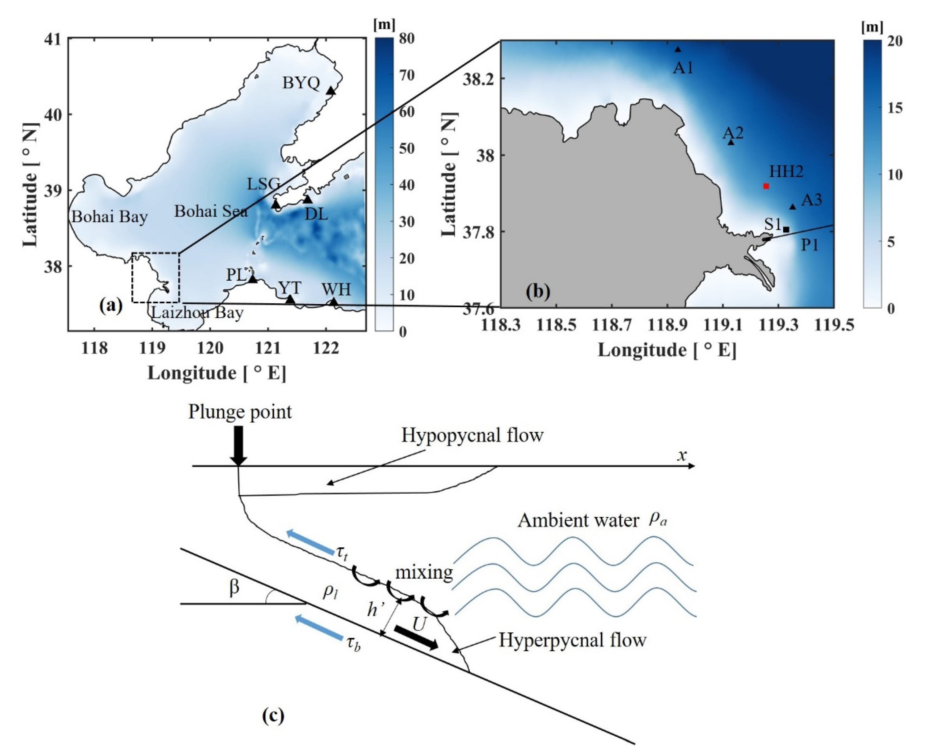
2.1. Hydrodynamic Model

The FVCOM is a three-dimensional hydrodynamic model that uses an unstructured, finite-element grid [40]. Compared to structured-grid models, the FVCOM’s unstructured grid is better for the YRE, which has a complex shoreline geometry and changes in its coastline. The model solves the three-dimensional momentum and conservation equations in integral form by computing fluxes between non-overlapping horizontal triangular control volumes. A σ-stretched coordinate system is applied in the vertical direction to improve the representation of the complicated bathymetry and obtain a smooth image of the irregular and variable bottom topography. Considering the high turbid nature of the YRE, the bottom boundary layer model (i.e., the BBL sediment model) was applied to the FVCOM because it considers sediment concentration, which influences the water density.

The suspended sediment model uses a concentration-based approach subject for the following evolution equation [41,42]:

$$\frac{\partial C}{\partial t}+\frac{\partial \left(uC\right)}{\partial x}+\frac{\partial \left(vC\right)}{\partial y}+\frac{\partial \left[\left(w-w_s\right)C\right]}{\partial z}=\frac{\partial }{\partial x}\left(A_H\frac{\partial C}{\partial x}\right)+\frac{\partial }{\partial y}\left(A_H\frac{\partial C}{\partial y}\right)+\frac{\partial }{\partial z}\left(K_h\frac{\partial C}{\partial z}\right)$$

(1)

where x, y, and z are the east, north, and vertical coordinates, respectively, whereas u, v, and w are the corresponding velocity components. C and w_s represent the sediment concentration and settling velocity, respectively, A_H is the horizontal eddy viscosity, and K_H is the vertical eddy viscosity. The Smagorinsky turbulence model was applied to the horizontal turbulence closure scheme [43], whereas the Mellor and Yamada level 2.5 turbulence closure scheme was adopted as the default for vertical viscosity [44]. Since Wright et al. [19] confirmed that the sediment concentration increases the density of the hyperpycnal flow above the ambient seawater, thus initiating plunging, the hyperpycnal flow density calculation should consider the effects of SSC. When the SSC is considered, the density of seawater ρ is calculated by a volumetric relationship developed by Winterwerp [45]:

$$\rho ={\rho }_w+\left(1-\frac{{\rho }_w}{{\rho }_s}\right)C$$

(2)

where ρ_w is the clear seawater density and ρ_s is the sediment density.

Sediment-induced stratification in the bottom boundary layer (BBL) reduces the vertical eddy viscosity [23] and the bottom shear stress compared to the model predictions in a neutrally stratified BBL [46]. Since this reduction in the vertical eddy viscosity and the bottom shear stress can significantly affect vertical sediment transport, we introduced the bottom drag coefficient (C_d) in a sediment-laden bottom boundary layer to consider the effects of water stratification [46,47]:

$$C_d=\frac{k^2}{{\left(1+A_1{R}_f\right)}^2{\left[\ln \left(\frac{h}{z_0}+1\right)-1\right]}^2}$$

(3)

where k = 0.4 is the von Karman constant, h is the water depth, and Z₀ is the bottom roughness parameter. A stability function considers the impact of stratification 1 + A₁R_f where A₁ is an empirical constant and R_f is the Richardson number. Following previous studies, A₁ = 5.5 was used for the sediment-laden oceanic bottom boundary layer [48].

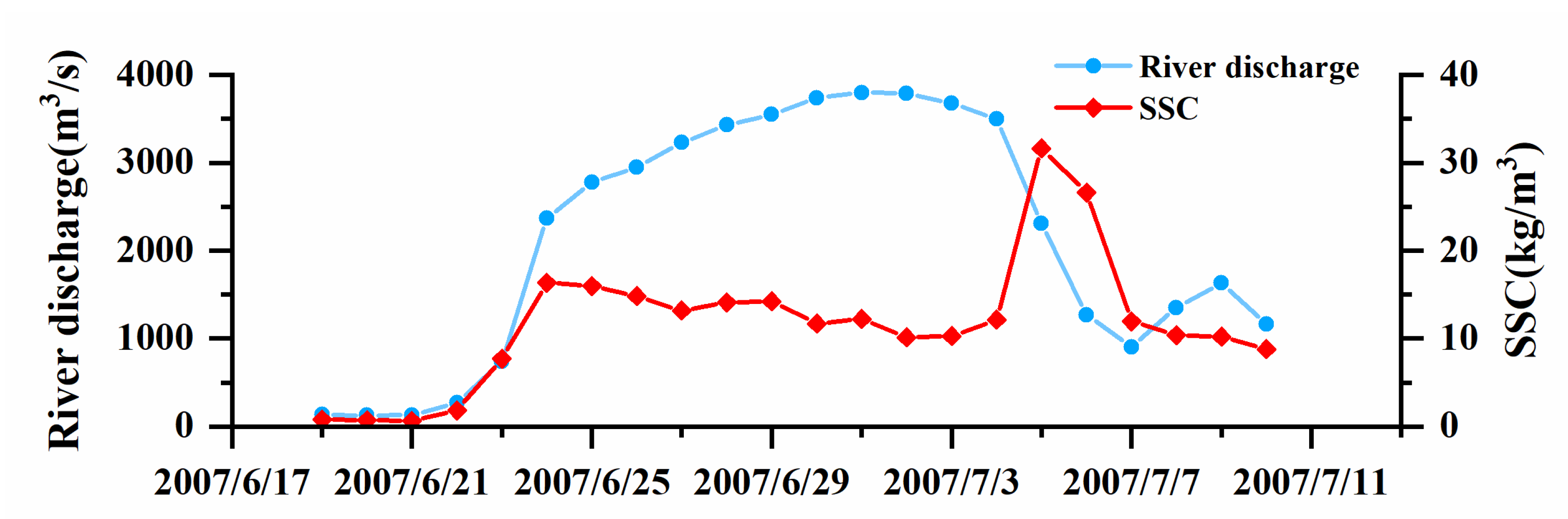
2.2. Model Configuration

The computation range of the model was 117.55° E–122.80° E, 37.14° N–41.02° N, spanning the whole Bohai Sea (Figure 1a). The unstructured triangular grids of the model domain consisted of 99,385 elements and 51,540 nodes, with the cell sizes of the elements ranging from 100 m on the nearshore of the YRE to 5 km at the open ocean boundary. Eleven sigma layers were specified in the vertical directions (σ = 0.0, −0.02, −0.08, −0.18, −0.32, −0.5, −0.68, −0.82, −0.92, −0.98, −1.0), with dense layers at the surface and the bottom levels to simulate the surface SSC and the SSC in the BBL.

The upstream inlet boundary used the water and sediment discharge at Lijin Station in 2007, and the model was driven by the tide forcing along the open boundary, consisting of 13 main tidal constituents M2, S2, N2, K2, K1, O1, P1, Q1, M4, MS4, MN4, MF, and MM. The model was initialized with a constant temperature and a salinity of 20 °C and 31.5 PSU, respectively, for the entire domain. The wind input data were obtained from the National Centers for Environmental Prediction’s (NCEP) Climate Forecast System version 2 (CFSv2). The model was launched with a cold start and ran from 25 June 2007 to 30 July 2007, forced with river discharges and tides. The vital parameters of the model are summarized in

Table 1. Key parameters of the model.

Parameters	Values
Sediment diameter	0.02 mm
Setting velocity	0.1 mm/s
Model time steps	3 s for the outer mode, 0.3 s for the internal mode
Bottom friction coefficient	Sediment-laden BBL
Horizontal diffusion	Smagorinsky scheme
Vertical eddy viscosity	M–Y 2.5 turbulent closure
Node, element, vertical layers	99,385 elements and 51,540 nodes (reference experiment 1), 11 vertical layers
Open boundary condition	Sea surface elevation time series from TPXO 7.2

.

2.3. Numerical Tests

The Water-Sediment Regulation Scheme (WSRS) lasted from 19 June to 3 July 2007. During this period, the maximum river discharge at Lijin Station was 3800 m³/s, with an average of about 2314 m³/s. The full sediment load was about 31.6 kg/m³, with an average of approximately 9.6 kg/m³, as shown in Figure 2. For easy calculation, the normal river discharge was taken as 4000 m³/s. The extreme river discharge was taken as 6000 m³/s to explore the influence of river discharges on the development process of sediment-laden hyperpycnal flows. Suspended sediment concentrations were taken as 15 kg/m³, 35 kg/m^3, and 85 kg/m³, to explore the influence of SSC on the formation and maintenance of sediment-laden hyperpycnal flows. It is noteworthy that although Cases 2 and 3 examined the influence of SSC on the formation and maintenance of hyperpycnal flows, Case 4 assessed the influence of high river discharge. Case 1 was used as the reference model in

Table 2. Details of the numerical experiments.

Experiments	Q (m3/s)	SSC (kg/m3)	Descriptions
Case 1	4000	85	Reference experiment
Case 2	4000	15	Analyze the influence of sediment concentration
Case 3	4000	35	Analyze the influence of sediment concentration
Case 4	6000	85	Analyze the influence of river discharge

below.

2.4. Definition of Important Parameters of Hyperpycnal Flow

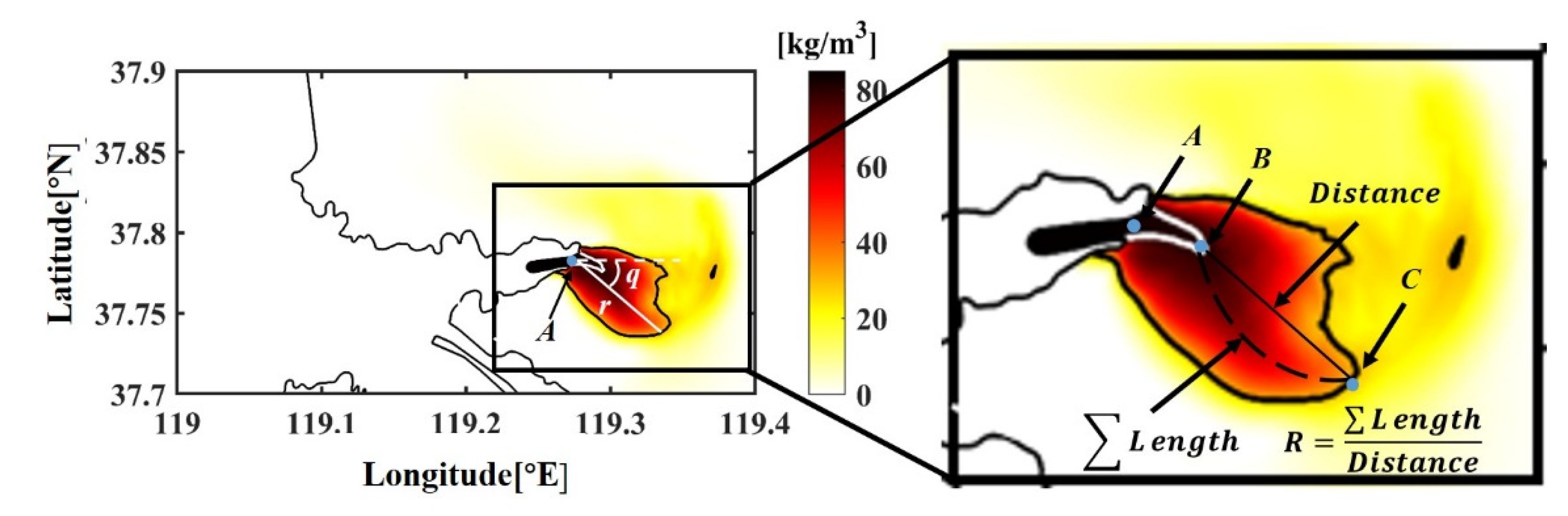
2.4.1. Path Index

To study the sediment hyperpycnal flow in the Yellow River Estuary, we defined the hyperpycnal flow path index (r, q) according to the distribution of the bottom SSC. As shown in Figure 3, the index r is the maximum distance between the river mouth and the SSC = 30 kg/m³ isoline; q is the runoff direction denoted by the angle between an eastward direction and the line linking the river mouth and the point corresponding to index r [49]. Furthermore, we used the curvature (R) to characterize the bending degree of the axis of the hyperpycnal flow. R is mathematically expressed as follows:

$$R=\frac{\sum Length}{Distance}$$

(4)

where $\sum Length$ is the curved distance between Points B and C, whereas Distance represents the straight distance between Points B and C (Figure 3). It should be noted that the curved line between Points B and C is the line linking all points on the isoline where the sediment concentration varies from 30 to 80 kg/m³ at the farthest from the river mouth, Point A.

2.4.2. Density

The basic condition for initiating sediment hyperpycnal flow is the plunging of high sediment-laden river waters into the estuary, which are driven downward by gravity (Figure 1c). The gravity difference enhances the downward flow of the fluid along the slope. Mathematically, gravity difference is expressed as:

$$g^{\prime }=g\left({\rho }_l-{\rho }_a\right)/{\rho }_a$$

(5)

where g is the acceleration of gravity, ${\rho }_l$ is the density of sediment density current, and ${\rho }_a$ is the density of the ambient water. In order to illustrate the density profiles, the excess bulk density ${\sigma }_{\mathrm{t}}$ is defined as follows:

$${\sigma }_{\mathrm{t}}=\rho -1000$$

(6)

where ρ is turbid seawater density.

2.4.3. Potential Energy

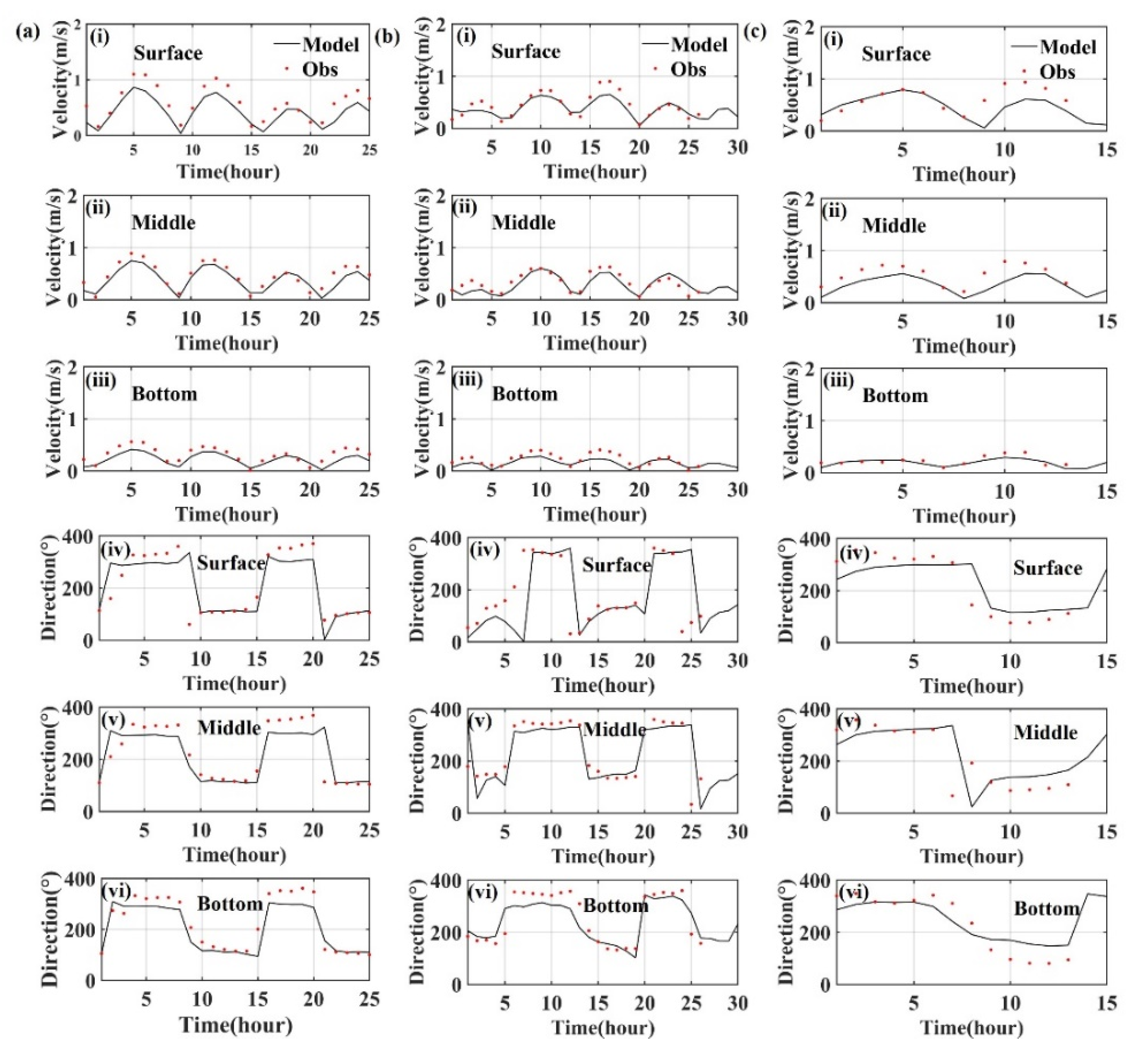
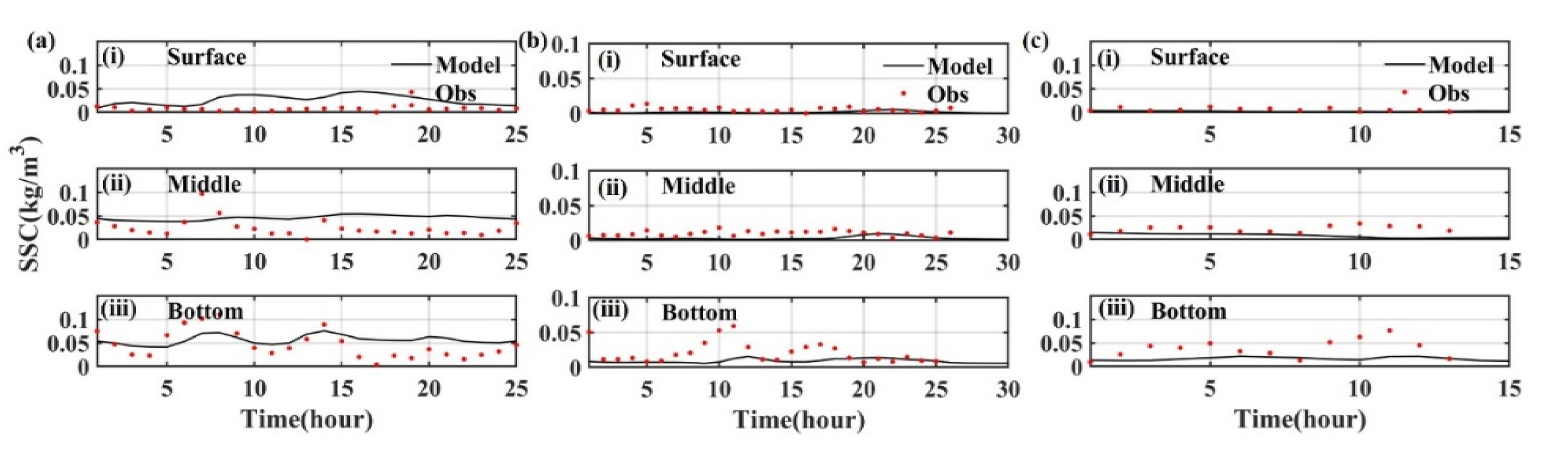
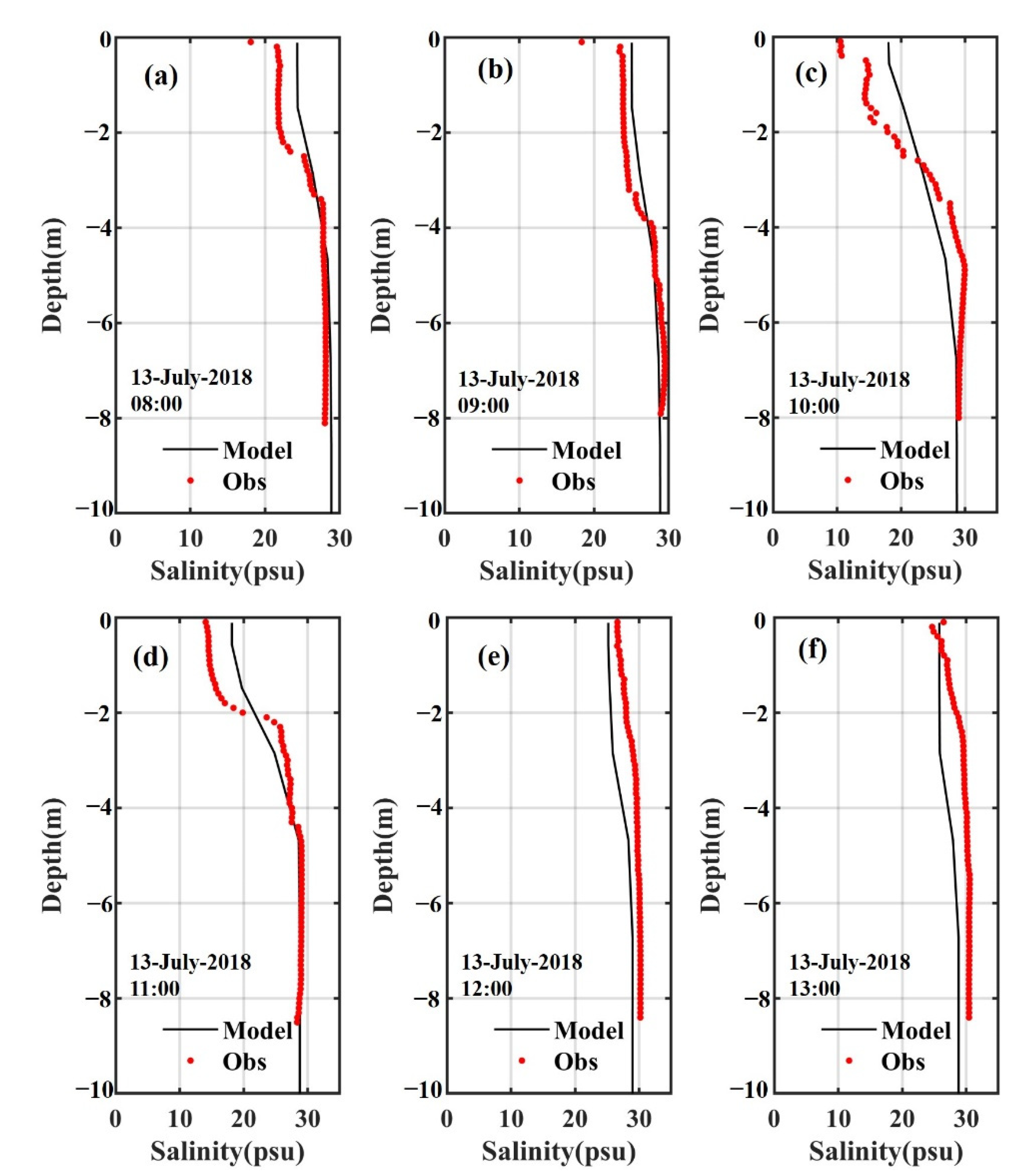
The alternation between vertical density mixing and stratification in water results from the transformation of kinetic energy and potential energy. The potential energy anomaly (ϕ), which is a very useful parameter in scaling the development and breakdown of stratification, has the following form [50,51]:

$$\phi =\frac{1}{h}{\int }_{-h}^0\left(\overline{\rho }-\rho \right)gzdz.$$

(7)

$$\overline{\rho }=\frac{1}{h}{\int }_{-h}^0\rho dz$$

(8)

Simpson et al. [52] hypothesized and proposed that four main mechanisms would affect $\varphi .$ tidal strain effect, gravity circulation effect, tidal stirring effect, and wind mixing effect. Thus, the time derivative of ϕ can be described by the following formula:

$$\begin{array}{l}\frac{\partial \varphi }{\partial t}={\left(\frac{\partial \varphi }{\partial t}\right)}_{\mathrm{strain} }+{\left(\frac{\partial \varphi }{\partial t}\right)}_{\mathrm{cir}}-{\left(\frac{\partial \varphi }{\partial t}\right)}_{\mathrm{stir}}-{\left(\frac{\partial \varphi }{\partial t}\right)}_{\mathrm{wind}}\\ =0.031gh{\overline{u}}_t\frac{\partial \rho }{\partial x}+0.0031\frac{g^2{h}^4}{A\rho }{\left(\frac{\partial \rho }{\partial x}\right)}^2-\epsilon k\rho \frac{|\overline{u}{|}^3}{h}-\delta k_s{\rho }_a\frac{{\overline{W}}^3}{h}\end{array}$$

(9)

In the above equation, the terms on the right-hand side represent the effects of tidal straining, gravitational circulation, tidal stirring, and wind stirring. $\overline{W}$ refers to wind speed, ρ_a is the density of air, and ${\overline{u}}_t$ denotes the depth-mean tidal current speed. The parameters $\epsilon$ = 0.0037 and $\delta$ = 0.023 are the mixing efficiencies. The effective drag coefficients for the bottom and surface stresses are denoted as $k$ and $k_s$, where typically $k$ = 2.5 × 10⁻³ and $k_s$ = 6.4 × 10⁻⁵ [51,52]. A is the vertical eddy diffusivity of turbulent momentum mixing.

3. Model Validation

The model was run with the water and sediment discharge at Lijin Station for two periods: from 25 June to 30 July 2007 and from 1 June to 15 July 2018. The simulation between 25 June and 30 July 2007 was used to validate the water levels, current velocities, directions, and SSC, whereas the simulation between 1 June and 15 July 2018 was used to validate the salinity near the YRE. To evaluate the model, two parameters, including correlation coefficients (CC) and skill scores (Skill), were calculated to quantify the differences between the field results and the simulation results. Equations for CC and Skill are presented as follows:

$$CC=\frac{1}{N}{\displaystyle \sum }_{i=1}^N\frac{\left(X_{\mathit{mod}}-{\overline{X}}_{\mathit{mod}}\right)\left(X_{obs}-{\overline{X}}_{obs}\right)}{S_m{S}_o}$$

(10)

$$\mathit{Skill}=1-\frac{{\displaystyle \sum _{i=1}^N}|X_{\mathit{mod}}-X_{obs}{|}^2}{{\displaystyle \sum _{i=1}^N}{(\left|X_{\mathit{mod}}-{\overline{X}}_{obs}|+|X_{obs}-{\overline{X}}_{obs}\right|)}^2}$$

(11)

where $X_{\mathit{mod}}$ and $X_{obs}$ are the model and observed values, with mean values ${\overline{X}}_{\mathit{mod}}$ and ${\overline{X}}_{obs}$, and standard deviations S_m and S_o, respectively. A value of CC or Skill near 1 indicates a close match between the observed and the model values.

The water level comparisons between model-generated results and tide gauge data are shown in Figure 4. Regarding the water levels at six tidal gauges, the difference between field observation data and model computations was calculated to be 9.0 cm, indicating the model reliably simulates the tide dynamics.

Figure 5a–c compare the velocity magnitude and flow directions between in situ observations and model computations at stations A1, A2, and A3, respectively. The results presented in

Table 3. Correlation coefficient and skill score of each measured site.

Stations	Velocity		Direction
	CC	Skill	CC	Skill
A1-sur	0.913	0.825	0.748	0.874
A1-mid	0.890	0.906	0.821	0.915
A1-bed	0.842	0.757	0.915	0.959
Ave	0.881	0.829	0.828	0.916
A2-sur	0.861	0.785	0.487	0.653
A2-mid	0.886	0.885	0.686	0.725
A2-bed	0.839	0.750	0.802	0.817
Ave	0.862	0.807	0.658	0.731
A3-sur	0.591	0.569	0.864	0.931
A3-mid	0.879	0.877	0.799	0.906
A3-bed	0.734	0.814	0.814	0.922
Ave	0.735	0.753	0.825	0.920

show that except for station A3, the average velocity values of CC and Skill reached 0.8. The table also revealed that except for group A2, the average direction values for Skill reached 0.9. Interestingly, the modeled velocity magnitude and the flow direction results significantly agree with the field observation data.

Figure 6a–c show that the verification results of SSC in each layer of the stations A1, A2, and A3 had the same order of magnitude as the measurements. The average skills of A1, A2, and A3 were 0.42, 0.56, and 0.44, respectively; thus, the efficiency of the sediment model is good. It is noteworthy that the modeled SSC values appear to be lower than the observed values because the input of the sediment from the oceanic boundary was not considered. Figure 7 displays modeled salinity profiles and cruise observations at HH2, indicating good agreements between modeled salinity profiles and cruise data.

4. Results

The dynamic characteristics of the hyperpycnal flow, as well as the influences of river discharge and sediment load on the formation and maintenance of the hyperpycnal flow, are illustrated using the parameters described in Section 2.4. Simulation results for maximum runoff distance (r), runoff direction (q), and curvature (R) are presented in

Table 4. Simulation results for maximum runoff distance (r), runoff direction (q), and curvature (R) in different cases. Note that parameters of Case 2 are not available because of its low sediment load. Since the SSC in Case 3 was less than 80 kg/m³, curvature (R) values are not available for Case 3.

Tidal Cycles	Parameters	Case 1	Case 3	Case 4
Peak Flood	Maximum Runoff Distance (r)	8.2 km	4.2 km	12.4 km
	Runoff Direction (q)	−18.5°	−31.6°	−3.4°
	Curvature (R)	1.17	-	1.19
Flood Slack	Maximum Runoff Distance (r)	8.1 km	3.7 km	11.1 km
	Runoff Direction (q)	4.6°	21.3°	7.0°
	Curvature (R)	2.23	-	2.03
Peak Ebb	Maximum Runoff Distance (r)	9.3 km	4.2 km	11.8 km
	Runoff Direction (q)	28.6°	59.8°	11.5°
	Curvature (R)	1.82	-	1.62
Ebb Slack	Maximum Runoff Distance (r)	9.3 km	4.7 km	11.8 km
	Runoff Direction (q)	55.5°	30.6°	46.8°
	Curvature (R)	1.35	-	1.37

.

In Table 4, runoff distance (r) and runoff direction (q) are used to characterize the runoff distance and direction of the hyperpycnal flow, respectively. The curvature (R) is used to characterize the bending degree of the runoff path such that the greater the R, the higher the curvature of the hyperpycnal flow runoff path.

It could be recalled from Table 2 that Case 1 had a river discharge of 4000 m³/s and a sediment load of 85 kg/m³, and Case 3 had a river discharge of 4000 m³/s and a sediment load of 35 kg/m³, whereas Case 4 had a river discharge of 6000 m³/s and a sediment load of 85 kg/m³. Based on the individual runoff distances stated above, the average runoff distance of hyperpycnal flows is about 8.7 km; the runoff ranged between −18.5° and 55.5°, whereas the average curvature R was approximately 1.64 for Case 1. For Case 4, the average runoff distance of hyperpycnal flow was about 11.8 km; the runoff ranged between −3.4° and 46.8°, whereas the average curvature was approximately 1.55 for Case 4.

Figure 8 presents the bottom suspended sediment concentrations at different times, which include peak flood, flood slack, peak ebb, and ebb slack in Cases 1 to 4. It can be observed that Cases 1 and 4 have white dash lines, which is the bending degree of the runoff path. The white dash line is a result of high sediment concentrations in these two cases. Conversely, it can be observed that Cases 2 and 3 do not have white dash lines due to low suspended concentrations, which were 15 kg/m³ and 35 kg/m³, respectively.

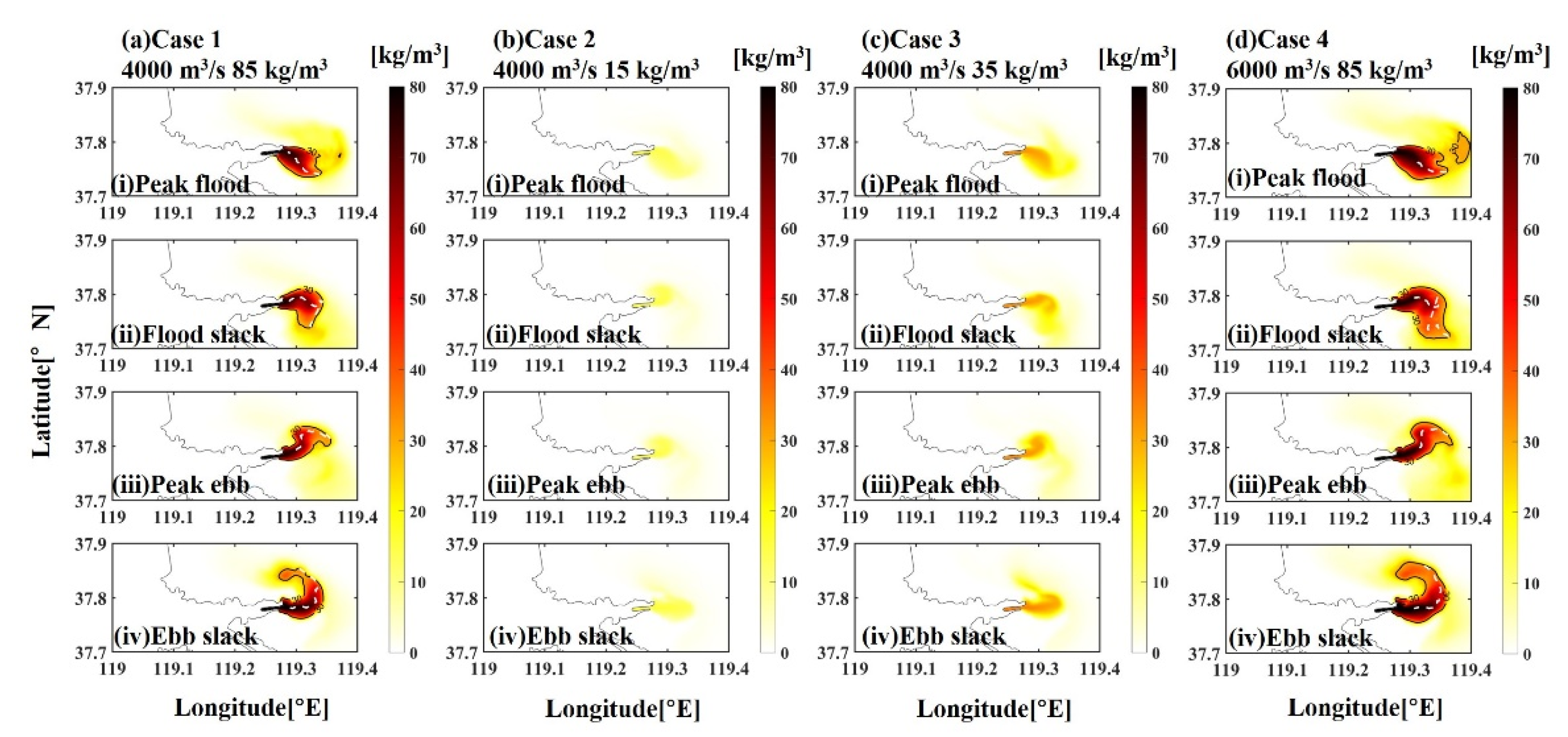
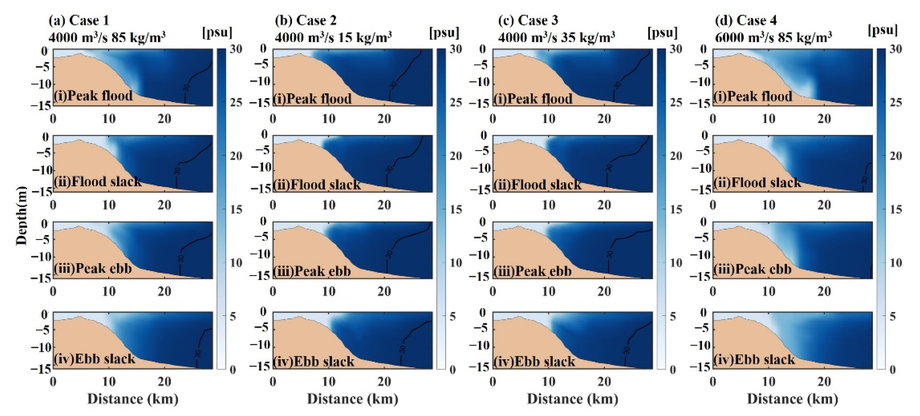
4.1. Variations of the Hyperpycnal Flow with Tides

In order to comprehensively explore the temporal and spatial characteristics of the development process of estuarine hyperpycnal flow, site S1 was chosen as the investigating site (see Figure 1b). On 2 July 2007, nine representative times were selected to study the development process. The vertical profiles of excess bulk density, SSC, salinity, and velocity are shown in Figure 9.

Figure 9a shows that the hyperpycnal layer (excess bulk density >20 kg/m³, SSC > 25 kg/m³) had a thickness of approximately 2.1 m at t = 0:00. The hyperpycnal layer had a salinity of less than 14 PSU, and the velocity of the hyperpycnal layer varied between 0.3 and 0.7 m/s. Later on, during the flood period from t = 1:00 to 2:00, as shown in Figure 9b,c, the thickness of the hyperpycnal layer gradually decreased to 1.5 m. The velocity of the hyperpycnal layer reduced, varying from 0.2–0.7 m/s, whereas the velocity above the hyperpycnal layer varied from 0.2–0.6 m/s.

At t = 4:00 (Figure 9d), the hyperpycnal layer thickness slightly decreased to approximately 1.4 m. The hyperpycnal layer had a salinity of approximately 8 PSU. During the ebb period from t = 5:00 to 6:00, as shown in Figure 9e,f, the thickness of the hyperpycnal layer increased back to ~2.1 m. The velocity above the hyperpycnal layer varied from −0.2–0.6 m/s, attributable to the ebb tidal current.

At t = 9:00 (Figure 9g), the hyperpycnal layer had a thickness of about 2.0 m, and its salinity was around 7 PSU. The maximum velocity was about 0.3 m/s, whereas the outflow velocity was approximately 0.1–0.25 m/s. At t = 10:00 (Figure 9h), the thickness of the hyperpycnal layer increased to about 2.4 m, and the salinity in the layer was about 6 PSU. The velocity in the layer was about 0.3–0.6 m/s. At t = 11:00 (Figure 9i), the thickness of the hyperpycnal layer continued to increase to about 3.0 m. At this time, the hyperpycnal flow was fully developed, and the salinity in the layer was about 6 PSU. The vertical distribution of salinity was relatively uniform, the current velocity in the layer was about 0.3–0.7 m/s, and the outflow velocity in the layer was about 0.4 m/s.

In summary, according to the results of the S1 station, the development process of the hyperpycnal flow was periodical with tidal cycles. As shown in

Table 5. Details of the numerical experiments.

Time	Tidal Cycles	Development Process
0:00	low slack water	fully developed
1:00	flood tide	thickness decreases
2:00	flood tide	thickness decreases
4:00	high slack water	thickness becomes thinnest
5:00	ebb tide	start to develop, thickness increases
6:00	ebb tide	thickness increases
9:00	peak ebb	thickness increases
10:00	ebb tide	thickness increases
11:00	low slack water	fully developed

, during the flood tide, the development of the hyperpycnal flow was limited, and the hyperpycnal layer gradually became thinner. At high slack water, the hyperpycnal layer became thinnest. During the ebb tidal stage, the hyperpycnal layer became thicker. At low slack water, the thickness of the hyperpycnal layer became thickest [5]. During the development process of the hyperpycnal flow, the bottom salinity decreased, and the SSC increased significantly when the hyperpycnal layer gradually became thicker. When the hyperpycnal layer gradually became thinner, the bottom salinity increased rapidly, and the SSC decreased.

4.2. Effects of River Sediment Load on Hyperpycnal Flows

In Case 2, the initial condition of the sediment load at the open boundary of the river side was set to 15 kg/m³ (see Table 2), which is lower than the critical concentration for hyperpycnal flow formation [6]. As shown in Figure 10b, the sediment load was insufficient to offset the density contrast induced by the salinity difference between the river water and ambient seawater in the YRE [7,10]. Therefore, the 15 kg/m³ sediment load cannot initiate the hyperpycnal flows. Figure 10b shows that the excess bulk density (σt) of the surface layer was roughly less than 10 kg/m³, and that of the near-bottom layer was approximately 20 kg/m³. The SSC varied with the interaction between tidal current and river discharge at different tidal moments, but the vertical profile was relatively uniform, measuring about 5–8 kg/m³, as shown in Figure 11b. Due to the similarity of excess density and salinity distributions, Figure 10b and Figure 12b demonstrate that the water column was nearly stratified by salinity. In contrast, the surface salinity was apparently lower than the bottom salinity.

In Case 3, the initial condition of the sediment load at the open boundary of the river side was set to 35 kg/m³ (see Table 2). As observed in Figure 10c, the excess bulk density (σt) was about 15–20 kg/m³, and there was only a weak density anomaly in the thin layer at the surface and bottom, with a slight trend of low-density density flow. Therefore, it can be reasonably inferred that 35 kg/m³ is near the critical concentration for hyperpycnal flow formation. Figure 11c and Figure 12c show that neither “saline wedge” nor “inverted saline wedge” was obvious, and the isolines of salinity and suspended sediment concentrations were slightly inclined.

In summary, when the sediment load is 15 kg/m³, the transport pathway of river sediment into the sea is mainly through the hypopycnal plume. Most of the sediment carried by freshwater floats above the seawater as a surface plume because its density is lower than the seawater density, making it difficult for the sediment-laden current to plunge into the estuary to form hyperpycnal flows [6,7,9]. However, when the river sediment load is 35 kg/m³, this concentration is high enough to overcome the increasing effect of salinity on density [10]. Therefore, hyperpycnal flows are formed.

4.3. Effects of River Discharge on Hyperpycnal Flows

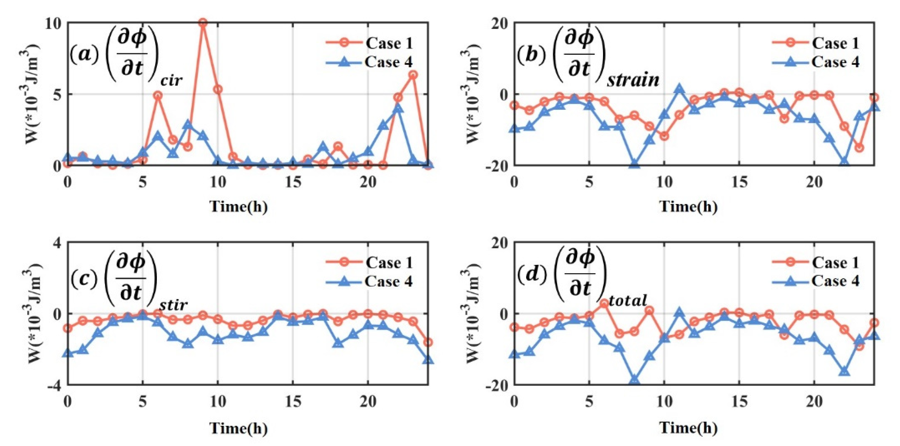
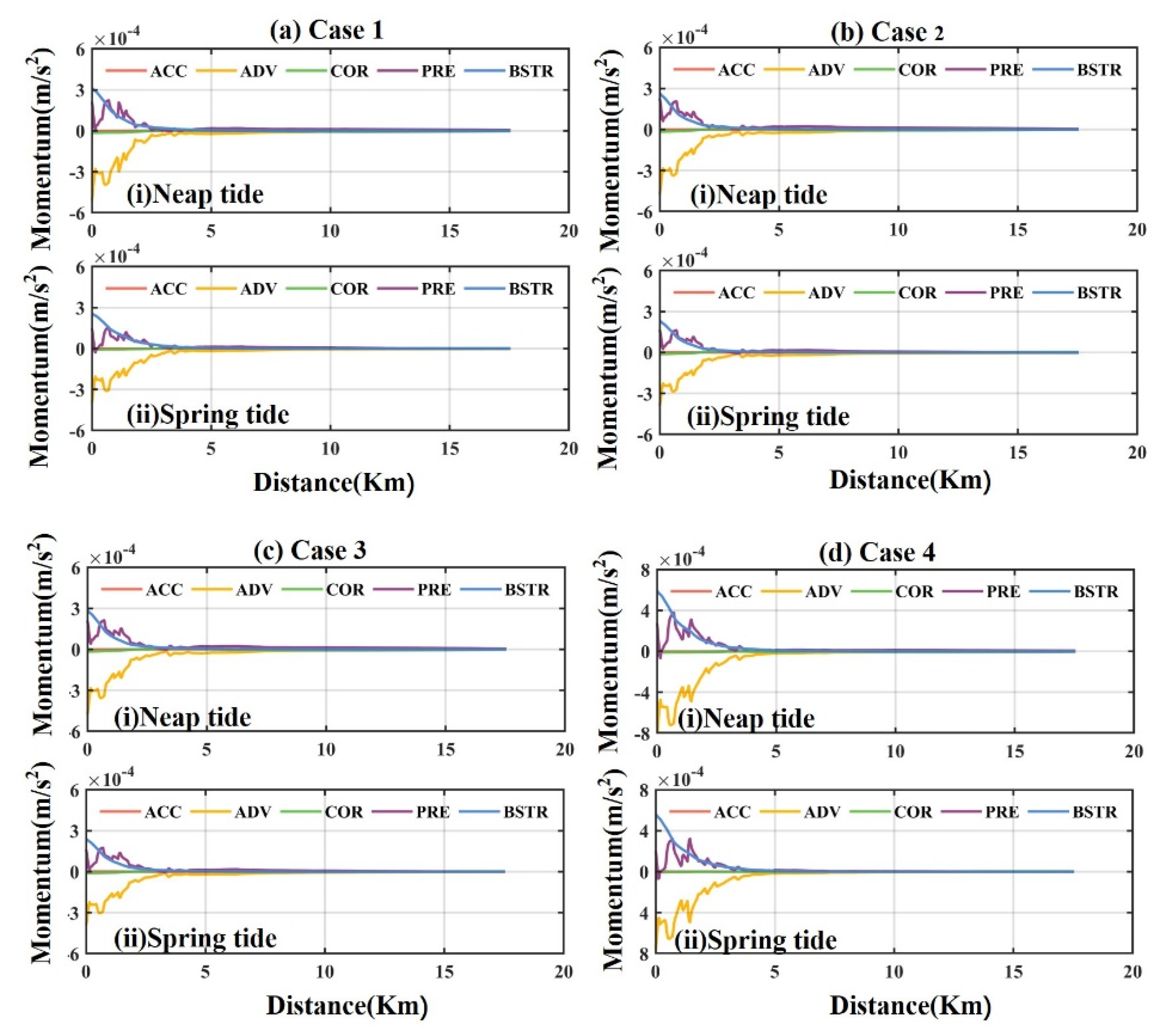
From the above average values in Table 4, it could be inferred that when the amount of river discharge increases, the runoff distance of hyperpycnal flow increases, the range of runoff direction decreases, and the bending degree of runoff path decreases.

Although Case 1 had a similar SSC as Case 4 (see Table 2), there was a significant difference in the river discharge where Case 1 had a river discharge of 4000 m³/s and Case 4 had a river discharge of 6000 m³/s. Comparing Figure 10a(iv),d(iv), which represent Cases 1 and 4, respectively, it can be inferred that the hypopycnal plume in Case 4 spread farther into the sea than in Case 1. This could be attributed to the higher river discharge in Case 4, which transported more freshwater to the open sea. Comparing Figure 12a,d, evidence of freshwater can be seen close to the bottom of the estuary in Case 4. This could be attributed to the higher river discharge and high sediment load. Interestingly, sediment loads in Cases 1 and 4 were similar. This established that high river discharge plays a significant role in hyperpycnal flow development. The above numerical experiments demonstrate that high river discharge plays an essential role in the formation and development of hyperpycnal flow. The larger the river discharge, the farther the hyperpycnal flow propagates to the open sea.

It was established that the development of hyperpycnal flow is closely related to the stratified mixing state of water volume [7]. To assess the stratification and mixing of the hyperpycnal flow during a tidal period, we chose station S1, which has a 3.6 m water depth (see Figure 1b), to study the stratification mechanism using Equation (9). Figure 13 presents the time-varying parameters of the water potential energy function at the S1 station. Figure 13a shows that the potential energy change rate, (∂ϕ/∂t)cir, was caused by gravitational circulation in Cases 1 and 4. It can be seen that in both cases, the (∂ϕ/∂t)cir is always greater than 0, meaning that river discharge promotes the stratification of the water column [48,49]. Figure 13b shows that the time derivative of ϕ induced by the tidal straining, (∂ϕ/∂t)strain, reached an average of −3.6× 10⁻³ W/m³ in Case 1 and an average of −6.6 × 10⁻³ W/m³ in Case 4. Figure 13c shows that the time derivative of ϕ induced by the tidal stirring, (∂ϕ/∂t)stir, had an average of −0.3 × 10⁻³ in Case 1, and an average of −1.1 × 10⁻³ in Case 4, which implies that (∂ϕ/∂t)stir promotes the mixing of the water column [50]. It is noteworthy that the total potential energy of gravitational circulation (Figure 13a), tidal straining (Figure 13b), and stirring (Figure 13c) are summed up and presented in Figure 13d. Under the combined effects of the above mechanisms, the average total time derivative of ϕ was −2.4 × 10⁻³ W/m³ for Case 1 and −6.8 × 10⁻³ W/m³ for Case 4 during the tidal period (see Figure 13d).

In summary, factors influencing the water structure mainly include gravitational circulation, tidal strain, and stirring [53]. The tidal strain is the main control factor of the periodic stratification-mixing process of hyperpycnal flows in the YRE.

5. Discussion

To evaluate the forcing mechanism of sediment transport when Yellow River runoff enters the sea, this study selected the axis section P1 of the estuary (see Figure 1b) and examined the variations in its momentum balance items along its course. According to Zu et al. [54], the momentum conservation equations can be written as follows:

$$\stackrel{1}{\overbrace{\frac{\partial U}{\partial t}}}=\stackrel{2}{\overbrace{U\frac{\partial U}{\partial x}+V\frac{\partial U}{\partial y}}}+\stackrel{3}{\overbrace{fV}}-\stackrel{4}{\overbrace{\frac{1}{{\rho }_0}\frac{\partial P}{\partial x}}}+\stackrel{5}{\overbrace{\frac{1}{{\rho }_{0}D}{\tau }_s^x}}-\stackrel{6}{\overbrace{\frac{1}{{\rho }_{0}D}{\tau }_b^x}}+\widetilde{F_x}$$

(12)

$$\frac{\partial V}{\partial t}=U\frac{\partial V}{\partial x}+V\frac{\partial V}{\partial y}-fU-\frac{1}{{\rho }_0}\frac{\partial P}{\partial y}+\frac{1}{{\rho }_{0}D}{\tau }_s^y-\frac{1}{{\rho }_{0}D}{\tau }_b^y+\widetilde{F_y}$$

(13)

where (U,V) are depth-averaged barotropic velocities in (x,y), f is the Coriolis parameter; ρ₀ is the reference density; P is depth-averaged pressure, D is the total water depth, (${\tau }_s^x$, ${\tau }_s^x$) are the surface wind stress components, (${\tau }_b^x$,${\tau }_b^y$) are the bottom stress components, and ($\widetilde{F_x}$,$\widetilde{F_y}$) represent horizontal viscosity terms. In the above equation, term 1 is the acceleration (ACC); term 2 is the nonlinear horizontal advection (ADV); term 3 is the Coriolis force (COR); term 4 is the pressure gradient force (PRE); term 5 is the surface wind stress (SSTR); and term 6 is the bottom stress (BSTR). The surface wind stress term and horizontal viscosity term were neglected in this study because of their small magnitudes.

It is worth mentioning that Figure 14b,c, as well as Figure 15b,c, showed when high-density hyperpycnal flow was not generated. Figure 15b,c present the mean-depth-averaged momentums in the alongshore section represented by the P1 location for 72 h. We observed that when high-density hyperpycnal flow was not developed in Case 2 and Case 3, the momentum terms at the initial location (i.e., distance = 0 km) in section P1 revealed the important role of the advection and bottom friction in the momentum balance in alongshore section P1. As the distance increased to 5 km, the momentum balance was dominated by the pressure gradient and advection. The effects of the tides may also influence the surrounding dynamics. Accordingly, the flow rate can be changed during spring-neap tidal circles [55,56]. When the distance was further extended to 10 km during the neap tide, the momentum balance was dominated by the pressure gradient, advection, and Coriolis force. Conversely, when the distance was further extended to 10 km during spring tide, the momentum balance was dominated by the pressure gradient and advection.

Figure 14a,d, as well as Figure 15a,d, show that high-density hyperpycnal flow was generated. When high-density hyperpycnal flow was developed in Case 1 and Case 4, the momentum terms at the initial location (distance = 0 km) in section P1 revealed that the advection and bottom friction play the most important role in the momentum balance. As the distance increased to 5 km, the momentum balance was dominated by the pressure gradient and advection. When the distance was further extended to 10 km, the results were still similar to Case 1 and 2. Basically, the present model result is reliable because the scale of the current in the YRE is not very large. Hence, the rotational effect induced by the Coriolis force is not very obvious [57]. The increasing river discharge mainly influenced the numerical value of the momentum balance term but does not evidently affect the dominant term of the momentum balance [58].

Our results from numerical experiments provide a reference on how the sediment dispersal system has been altered in the estuary of a large river (e.g., the Amazon River) and build a linkage between the drainage process and sediment dynamics in the estuary [3].

6. Conclusions

A 3-D, hydrodynamic and sediment transport numerical model was developed and calibrated to study the formation and development of hyperpycnal flows in the YRE. The main conclusions are as follows:

The SSC transported by the river discharge is of primary importance to the formation of hyperpycnal flows. The sediment hyperpycnal flow in the YRE is formed when the fine sediment load in the river discharge is high enough (>30~40 kg/m³) to overcome the seawater salinity. If the fine sediment load is low (i.e., less than ~15 kg/m³), the surface hypopycnal flow occurs to transport sediment into the YRE. The hyperpycnal flow periodically varies with the tidal cycles in the bottom layer. The hyperpycnal flow evolves rapidly at the ebb tide and develops sufficiently at low slack waters before its gradual decay. During the flood tide, the hyperpycnal flow and its thickness continue to decrease. The main control factors of momentum balance differ with the transport positions of the sediment hyperpycnal flow. The nonlinear advection term and pressure gradient term are the main control items in the whole transport process, which significantly impact the dynamic characteristics.

The study also revealed that river discharge is important in maintaining the hyperpycnal flow in the estuary. With the increase in the river discharge, the propagating distance increased, and the propagating range of the hyperpycnal flow was reduced. The Simpson potential energy theory analysis shows that gravitational circulation intensifies the stratification, whereas tidal stirring promotes the mixing in the YRE. Tidal straining promotes the mixing during the flood tide and enhances the stratification during the ebb tide. The tidal straining is the main control factor of the periodic stratification-mixing process of hyperpycnal flows in the YRE. This study provides valuable information on the hyperpycnal flow variations with tides, river discharges, and sediment loads for future research in the YRE. Furthermore, the findings from this study can provide scientific explanations for the mechanism of suspended sediment dynamics in the YRE.

References

1. Shanmugam, G. Global significance of wind forcing on deflecting sediment plumes at river mouths: Implications for hyperpycnal flows, sediment transport, and provenance. J. Indian Assoc. Sedimentol. 2019, 36, 1–37. [Google Scholar]
2. Wright, L.D.; Friedrichs, C.T. Gravity-driven sediment transport on continental shelves: A status report. Cont. Shelf Res. 2006, 26, 2092–2107. [Google Scholar] [CrossRef]
3. Shi, F.; Chickadel, C.C.; Hsu, T.J.; Kirby, J.T.; Farquharson, G.; Ma, G. High-resolution non-hydrostatic modeling of frontal features in the mouth of the Columbia River. Estuar Coast. 2017, 40, 296–309. [Google Scholar] [CrossRef]
4. Wang, H.; Bi, N.; Wang, Y.; Saito, Y.; Yang, Z. Tide-modulated hyperpycnal flows off the Huanghe (Yellow River) mouth, China. Earth Surf. Process. Landf. 2010, 35, 1315–1329. [Google Scholar] [CrossRef]
5. Bates, C.C. Rational theory of delta formation. Aapg Bull. 1953, 37, 2119–2162. [Google Scholar]
6. Khan, S.M.; Imran, J.; Bradford, S.; Syvitski, J. Numerical modeling of hyperpycnal plume. Mar. Geol. 2005, 222, 193–211. [Google Scholar] [CrossRef]
7. Wang, Y.; Wang, H.; Bi, N.; Yang, Z. Numerical modeling of hyperpycnal flows in an idealized river mouth. Estuar. Coast. Shelf Sci. 2011, 93, 228–238. [Google Scholar] [CrossRef]
8. Zhao, L.; Ouillon, R.; Vowinckel, B.; Meiburg, E.; Kneller, B.; He, Z. Transition of a Hyperpycnal Flow Into a Saline Turbidity Current Due to Differential Diffusivities. Geophys. Res. Lett. 2018, 45, 11875–11884. [Google Scholar] [CrossRef] [Green Version]
9. Shanmugam, G. Mass Transport, Gravity Flows, and Bottom Currents: Downslope and Alongslope Processes and Deposits; Elsevier: Amsterdam, The Netherlands, 2020. [Google Scholar]
10. Mulder, T.; Syvitski, J.P.M. Turbidity currents generated at river mouths during exceptional discharges to the world oceans. J. Geol. 1995, 103, 285–299. [Google Scholar] [CrossRef]
11. Forel, F.A. Le Léman: Monographie Limnologique; F. Rouge: Dearborn, MI, USA, 1892. [Google Scholar]
12. Bhattacharya, J.P.; MacEachern, J.A. Hyperpycnal rivers and prodeltaic shelves in the Cretaceous seaway of North America. J. Sediment. Res. 2009, 79, 184–209. [Google Scholar] [CrossRef]
13. Gihm, Y.S.; Hwang, I.G. Lacustrine hyperpycnal flow deposits after explosive volcanic eruptions, Cretaceous Beolkeum Member, Wido Island, Korea. Geosci. J. 2016, 20, 157–166. [Google Scholar] [CrossRef]
14. Collins, D.S.; Johnson, H.D.; Allison, P.A.; Guilpain, P.; Damit, A.R. Coupled ‘storm-flood’depositional model: Application to the Miocene–Modern Baram Delta Province, north-west Borneo. Sedimentology 2017, 64, 1203–1235. [Google Scholar] [CrossRef] [Green Version]
15. Pan, S.; Liu, H.; Zavala, C.; Liu, C.; Liang, S.; Zhang, Q.; Bai, Z. Sublacustrine hyperpycnal channel-fan system in a large depression basin: A case study of Nen 1 Member, Cretaceous Nenjiang Formation in the Songliao Basin, NE China. Pet. Explor. Dev. 2017, 44, 911–922. [Google Scholar] [CrossRef]
16. Ford, D.E.; Johnson, M.C. An Assessment of Reservoir Density Currents and Inflow Processes; Technical Report E-83-7; United States Army Engineer Waterways Experiment Station: Vicksburg, MS, USA, 1983. [Google Scholar]
17. Mulder, T.; Syvitski, J.P.M.; Migeon, S.; Faugères, J.-C.; Savoye, B. Marine hyperpycnal flows: Initiation, behavior and related deposits. A review. Mar. Pet. Geol. 2003, 20, 861–882. [Google Scholar] [CrossRef]
18. Mountjoy, J.J.; Howarth, J.D.; Orpin, A.R.; Barnes, P.M.; Bowden, D.A.; Rowden, A.A.; Schimel, A.C.; Holden, C.; Horgan, H.J.; Nodder, S.D.; et al. Earthquakes drive large-scale submarine canyon development and sediment supply to deep-ocean basins. Sci. Adv. 2018, 4, eaar3748. [Google Scholar] [CrossRef] [PubMed] [Green Version]
19. Wright, L.D.; Wiseman, W.J.; Bornhold, B.D.; Prior, D.B.; Suhayda, J.N.; Keller, G.H.; Yang, Z.-S.; Fan, Y.B. Marine dispersal and deposition of Yellow River silts by gravity-driven underflows. Nature 1988, 332, 629–632. [Google Scholar] [CrossRef]
20. Wang, H.; Bi, N.; Saito, Y.; Wang, Y.; Sun, X.; Zhang, J.; Yang, Z. Recent changes in sediment delivery by the Huanghe (Yellow River) to the sea: Causes and environmental implications in its estuary. J. Hydrol. 2010, 391, 302–313. [Google Scholar] [CrossRef]
21. Lamb, M.P.; Mohrig, D. Do hyperpycnal-flow deposits record river-flood dynamics? Geology 2009, 37, 1067–1070. [Google Scholar] [CrossRef]
22. Snow, K.; Sutherland, B.R. Particle-laden flow down a slope in uniform stratification. J. Fluid Mech. 2014, 755, 251–273. [Google Scholar] [CrossRef] [Green Version]
23. He, Z.; Zhao, L.; Lin, T.; Hu, P.; Lv, Y.; Ho, H.-C.; Lin, Y.-T. Hydrodynamics of Gravity Currents down a Ramp in Linearly Stratified Environments. J. Hydraul. Eng. 2017, 143, 04016085. [Google Scholar] [CrossRef]
24. Wilson, R.I.; Friedrich, H.; Stevens, C. Turbulent entrainment in sediment-laden flows interacting with an obstacle. Phys. Fluids 2017, 29, 036603. [Google Scholar] [CrossRef]
25. Zordan, J.; Juez, C.; Schleiss, A.J.; Franca, M.J. Entrainment, transport and deposition of sediment by saline gravity currents. Adv. Water Resour. 2018, 115, 17–32. [Google Scholar] [CrossRef]
26. He, Z.; Zhu, R.; Zhao, L.; Chen, J.; Lin, Y.-T.; Yuan, Y. Hydrodynamics of weakly and strongly stratified two-layer lock-release gravity currents. J. Hydraul. Res. 2021, 59, 989–1003. [Google Scholar] [CrossRef]
27. Wang, X.H.; Wang, H. Tidal straining effect on the suspended sediment transport in the Huanghe (Yellow River) Estuary, China. Ocean Dyn. 2010, 60, 1273–1283. [Google Scholar] [CrossRef]
28. Wright, L.D.; Wiseman, W.J., Jr.; Yang, Z.S.; Bornhold, B.D.; Keller, G.H.; Prior, D.B.; Suhayda, J.N. Processes of marine dispersal and deposition of suspended silts off the modern mouth of the Huanghe (Yellow River). Cont. Shelf Res. 1990, 10, 1–40. [Google Scholar] [CrossRef]
29. Peakall, J.; Kane, I.A.; Masson, D.G.; Keevil, G.; McCaffrey, W.; Corney, R. Global (latitudinal) variation in submarine channel sinuosity. Geology 2012, 40, 11–14. [Google Scholar] [CrossRef]
30. Davarpanah Jazi, S.; Wells, M.G.; Peakall, J.; Dorrell, R.M.; Thomas, R.E.; Keevil, G.M.; Darby, S.E.; Sommeria, J.; Viboud, S.; Valran, T. Influence of Coriolis force upon bottom boundary layers in a large-scale gravity current experiment: Implications for evolution of sinuous deep-water channel systems. J. Geophys. Res. Ocean. 2020, 125, e2019JC015284. [Google Scholar] [CrossRef]
31. Tseng, C.-Y.; Chou, Y.-J. Nonhydrostatic simulation of hyperpycnal river plumes on sloping continental shelves: Flow structures and nonhydrostatic effect. Ocean Model. 2018, 124, 33–47. [Google Scholar] [CrossRef]
32. Yu, J.; Fu, Y.; Li, Y.; Han, G.; Wang, Y.; Zhou, D.; Sun, W.; Gao, Y.; Meixner, F.X. Effects of water discharge and sediment load on evolution of modern Yellow River Delta, China, over the period from 1976 to 2009. Biogeosciences 2011, 8, 2427–2435. [Google Scholar] [CrossRef] [Green Version]
33. Milliman, J.D. River inputs. In Encyclopedia of Ocean Sciences; Steele, J.H., Turekian, K.K., Thorpe, S.A., Eds.; Academic Press: Cambridge, UK; London, UK, 2001; Volume 4, pp. 2419–2427. [Google Scholar]
34. Milliman, J.D.; Meade, R.H. World-wide delivery of river sediment to the oceans. J. Geol. 1983, 91, 1–21. [Google Scholar] [CrossRef]
35. Chen, S.-N.; Geyer, W.R.; Hsu, T.-J. A numerical investigation of the dynamics and structure of hyperpycnal river plumes on sloping continental shelves. J. Geophys. Res. Oceans 2013, 118, 2702–2718. [Google Scholar] [CrossRef]
36. Bi, N.; Wang, H.; Yang, Z. Recent changes in the erosion–accretion patterns of the active Huanghe (Yellow River) delta lobe caused by human activities. Cont. Shelf Res. 2014, 90, 70–78. [Google Scholar] [CrossRef]
37. Wu, X.; Bi, N.; Yuan, P.; Li, S.; Wang, H. Sediment dispersal and accumulation off the present Huanghe (Yellow River) delta as impacted by the Water-Sediment Regulation Scheme. Cont. Shelf Res. 2015, 111, 126–138. [Google Scholar] [CrossRef]
38. Fan, Y.; Chen, S.; Pan, S.; Dou, S. Storm-induced hydrodynamic changes and seabed erosion in the littoral area of Yellow River Delta: A model-guided mechanism study. Cont. Shelf Res. 2020, 205, 104171. [Google Scholar] [CrossRef]
39. Ji, H.; Pan, S.; Chen, S. Impact of river discharge on hydrodynamics and sedimentary processes at Yellow River Delta. Mar. Geol. 2020, 425, 106210. [Google Scholar] [CrossRef]
40. Chen, C.; Liu, H.; Beardsley, R.C. An unstructured grid, finite-volume, three-dimensional, primitive equations ocean model: Application to coastal ocean and estuaries. J. Atmos. Ocean. Technol. 2003, 20, 159–186. [Google Scholar] [CrossRef]
41. Wu, L.; Chen, C.; Guo, P.; Shi, M.; Qi, J.; Ge, J. A FVCOM-based unstructured grid wave, current, sediment transport model, I. Model description and validation. J. Ocean Univ. China 2011, 10, 1–8. [Google Scholar] [CrossRef]
42. Warner, J.C.; Sherwood, C.R.; Signell, R.P.; Harris, C.K.; Arango, H.G. Development of a three-dimensional, regional, coupled wave, current, and sediment-transport model. Comput. Geosci. 2008, 34, 1284–1306. [Google Scholar] [CrossRef]
43. Smagorinsky, J. General circulation experiments with the primitive equations: I. The basic experiment. Mon. Weather Rev. 1963, 91, 99–164. [Google Scholar] [CrossRef]
44. Mellor, G.L.; Yamada, T. Development of a turbulence closure model for geophysical fluid problems. Rev. Geophys. 1982, 20, 851–875. [Google Scholar] [CrossRef] [Green Version]
45. Winterwerp, J.C. Stratification effects by cohesive and noncohesive sediment. J. Geophys. Res. Ocean. 2001, 106, 22559–22574. [Google Scholar] [CrossRef] [Green Version]
46. Wang, X.H. Tide-induced sediment resuspension and the bottom boundary layer in an idealized estuary with a muddy bed. J. Phys. Oceanogr. 2002, 32, 3113–3131. [Google Scholar] [CrossRef]
47. Wang, X.H.; Byun, D.S.; Wang, X.L.; Cho, Y.K. Modelling tidal currents in a sediment stratified idealized estuary. Cont. Shelf Res. 2005, 25, 655–665. [Google Scholar] [CrossRef]
48. Adams, C.E., Jr.; Weatherly, G.L. Some effects of suspended sediment stratification on an oceanic bottom boundary layer. J. Geophys. Res. Ocean. 1981, 86, 4161–4172. [Google Scholar] [CrossRef]
49. Wang, Q.; Guo, X.; Takeoka, H. Seasonal variations of the Yellow River plume in the Bohai Sea: A model study. J. Geophys. Res. Earth Surf. 2008, 113, C08046. [Google Scholar] [CrossRef]
50. Simpson, J.H.; Allen, C.M.; Morris, N.C.G. Fronts on the continental shelf. J. Geophys. Res. Ocean. 1978, 83, 4607. [Google Scholar] [CrossRef]
51. Simpson, J.H.; Bowers, D. Models of stratification and frontal movement in shelf seas. Deep.-Sea Res. Part I-Oceanogr. Res. Pap. 1981, 28, 727–738. [Google Scholar] [CrossRef]
52. Simpson, J.H.; Brown, J.; Matthews, J.; Allen, G. Tidal straining, density currents, and stirring in the control of estuarine stratification. Estuaries 1990, 13, 125–132. [Google Scholar] [CrossRef]
53. Li, L.; He, Z.; Xia, Y.; Dou, X. Dynamics of sediment transport and stratification in Changjiang River Estuary, China. Estuar. Coast. Shelf Sci. 2018, 213, 1–17. [Google Scholar] [CrossRef]
54. Zu, T.; Gan, J. A numerical study of coupled estuary–shelf circulation around the Pearl River Estuary during summer: Responses to variable winds, tides and river discharge. Deep-Sea Res. Part II 2015, 117, 53–64. [Google Scholar] [CrossRef]
55. Chen, Z.; Jiang, Y.; Liu, J.T.; Gong, W. Development of upwelling on pathway and freshwater transport of Pearl River plume in northeastern South China Sea. J. Geophys. Res. Ocean. 2017, 122, 6090–6109. [Google Scholar] [CrossRef]
56. Yu, X.; Guo, X.; Gao, H.; Zou, T. Upstream extension of a bottom-advected plume and its mechanism: The case of the Yellow River. J. Phys. Oceanogr. 2021, 51, 2351–2371. [Google Scholar] [CrossRef]
57. Zheng, S.; Guan, W.; Cai, S.; Wei, X.; Huang, D. A model study of the effects of river discharges and interannual variation of winds on the plume front in winter in Pearl River Estuary. Cont. Shelf Res. 2014, 73, 31–40. [Google Scholar] [CrossRef]
58. Pan, J.; Gu, Y.; Wang, D. Observations and numerical modeling of the Pearl River plume in summer season. J. Geophys. Res. Ocean. 2014, 119, 2480–2500. [Google Scholar] [CrossRef]
Figure 1. (a) Computational domain and locations of tide gauges along the Bohai coast, where six triangles represent six gauges, namely: DL (Dalian), LSG (Lvshungang), BYQ (Bayuquan), PL (Penglai), YT (Yantai) and WH (Weihai). (b) Locations of study sites near the Yellow River Estuary. Note: the black triangles indicate the locations of hydrosediment measurement stations (i.e., A1, A2, and A3); the red squares denote the location of the salinity measurement stations HH2; the black squares indicate the position of station S1 along the flow direction of the Yellow River into the open sea, whereas the black line indicates the position of section P1 which is along the flow direction of the Yellow River into the open sea. (c) A cross-section diagram showing hypopycnal flow along the surface and hyperpycnal flow along the bottom of an estuary.
Jmse 10 00943 g001
Figure 2. Daily river discharges and SSC at Lijin station between 19 June and 10 July 2007.
Jmse 10 00943 g002
Figure 3. Path index of the hyperpycnal flow. Index r is the maximum distance between Point A and Point B; q is the runoff direction denoted by the angle between the eastward direction (i.e., white dash lines) and the line linking Points A and B. Note that Point A is the river mouth, Point B is the position on the isoline where SSC = 80 kg/m3, whereas Point C is the position on the isoline where SSC = 30 kg/m3. R is the curved distance between Points B and C divided by the straight distance between Points B and C.
Jmse 10 00943 g003
Figure 4. The comparison between computed (red dots) and measured (black solid line) water levels at different stations. (a) Bayuquan, (b) Dalian, (c) Lvshungang, (d) Penglai, (e) Weihai, and (f) Yantai.
Jmse 10 00943 g004
Figure 5. The comparison between computed (red dots) and measured currents (black solid line): (a) represents station A1, the time is in hours from 10:00 on 4 July 2007 to 10:00 on 5 July 2007; (b) represents station A2, the time is in hours from 06:00 on 3 July 2007 to 07:00 on 4 July 2007; (c) represents station A3, the time is in hours from 10:00 on 29 June 2007 to 22:00 on 29 June 2007. (i) Surface current velocity; (ii) middle current velocity; (iii) bottom current velocity; (iv) surface current direction; (v) middle current direction; (vi) bottom current direction.
Jmse 10 00943 g005
Figure 6. The comparison between computed (red dots) and measured SSC (black solid line): (a) represents station A1, the time is in hours from 10:00 on 4 July 2007 to 10:00 on 5 July 2007; (b) represents station A2, the time is in hours from 06:00 on 3 July 2007 to 07:00 on 4 July 200; (c) represents station A3 the time is in hours from 10:00 on 29 June 2007 to 22:00 on 29 June 2007. (i) Surface suspended sediment concentration; (ii) middle suspended sediment concentration; (iii) bottom suspended sediment concentration.
Jmse 10 00943 g006
Figure 7. The comparison between computed and measured salinity. The time is in hours from 08:00 to 13:00 (af) on 13 July 2018.
Jmse 10 00943 g007
Figure 8. Bottom SSC at different times for different cases (ad) representing Case 1–4, respectively: (i) peak flood; (ii) flood slack; (iii) peak ebb; (iv) ebb slack. Note that Case 1 is the reference case and the white dash lines in the figures connects the point on the isoline where the sediment concentration varies from 30 to 80 kg/m3 at the farthest distance from the river mouth. Note that there are no white lines in Figure 8b,c, which represent Cases 2 and 3, respectively, because the SSC in these two cases were less than 80 kg/m3.
Jmse 10 00943 g008
Figure 9. Vertical profiles of excess bulk density (sigma-t), suspended sediment concentration (SSC), salinity (sal), and velocity (vel) in the station S1 at different times. Note that station S1 is shown in Figure 1b and the black dash lines indicate the hyperpycnal layer. (a) 00:00 (b) 01:00 (c) 02:00 (d) 04:00 (e) 05:00 (f) 06:00 (g) 09:00 (h) 10:00 (i) 11:00 on 2 July 2007.
Jmse 10 00943 g009
Figure 10. Vertical profiles of excess bulk density along the axial section P1 at different times: Note that Figure 10a–d represent Case 1–4, respectively whereas (i) peak flood; (ii) flood slack; (iii) peak ebb; (iv) ebb slack.
Jmse 10 00943 g010
Figure 11. Vertical profiles of SSC along the axial section P1 at different times: Note that Figure 11a–d represent Case 1–4, respectively whereas (i) peak flood; (ii) flood slack; (iii) peak ebb; (iv) ebb slack.
Jmse 10 00943 g011
Figure 12. Vertical profiles of salinity along the axial section P1 at different times: Note that Figure 12a–d represent Case 1–4, respectively whereas (i) peak flood; (ii) flood slack; (iii) peak ebb; (iv) ebb slack.
Jmse 10 00943 g012
Figure 13. Time series of the derivatives of the potential energy due to (a) gravitational circulation ((∂ϕ/∂t)cir), (b) tidal straining ((∂ϕ/∂t)strain), (c) tidal stirring ((∂ϕ/∂t)stir), and (d) total time derivative of the potential energy anomaly ((∂ϕ/∂t)total) using Equation (9) on 2 July at station S1 shown in Figure 1b.
Jmse 10 00943 g013
Figure 14. Depth-averaged terms in the 2-D momentum balance equations [i.e., Equation (12)] during six tidal cycles (~72 h) at section P1. (a) Case 1, (b) Case 2, (c) Case 3, and (d) Case 4.
Jmse 10 00943 g014
Figure 15. Contribution of each term to momentum during spring tide and neap tide: (i–iii) means during neap tide, distance = 0, 5, 10 km; (ivvi) means during spring tide, distance = 0, 5, 10 km. (a) Case 1, (b) Case 2, (c) Case 3, and (d) Case 4.
Jmse 10 00943 g015