
Verification of an Environmental Impact Assessment Using a Multivariate Statistical Model


 ,
,  ,
, 
Abstract
:1. Introduction
2. Materials and Methods
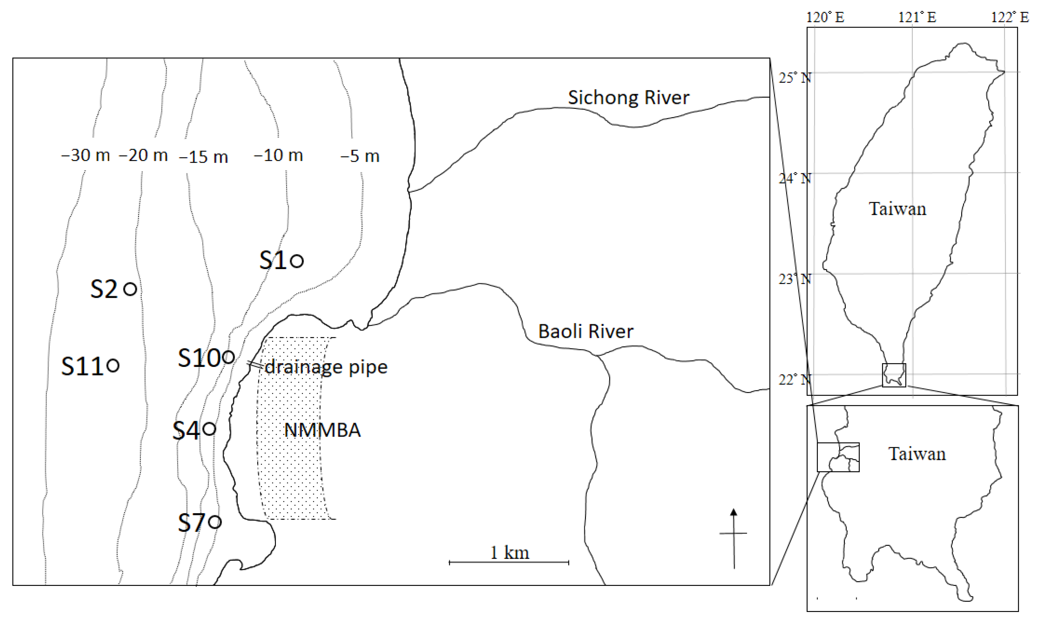
2.1. Study Area
2.2. Measurement of Abiotic and Biotic Parameters
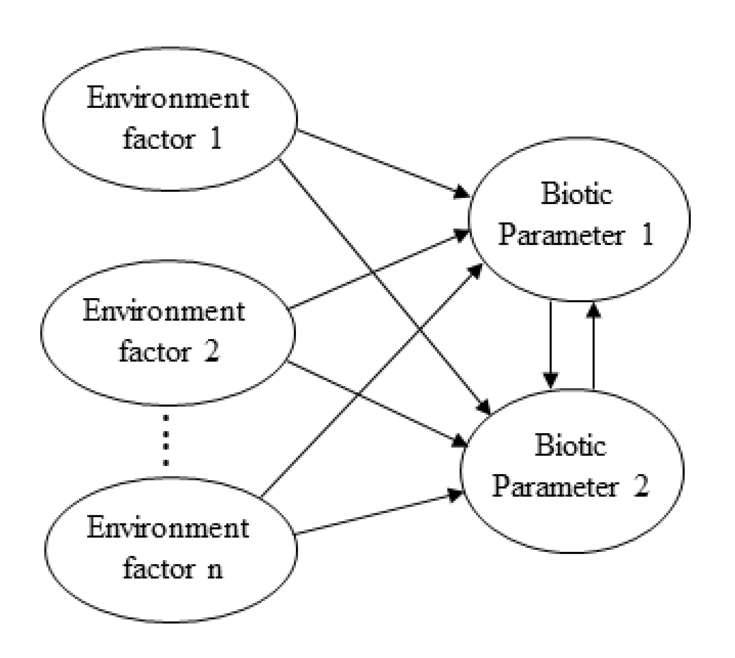
2.3. Data Analysis
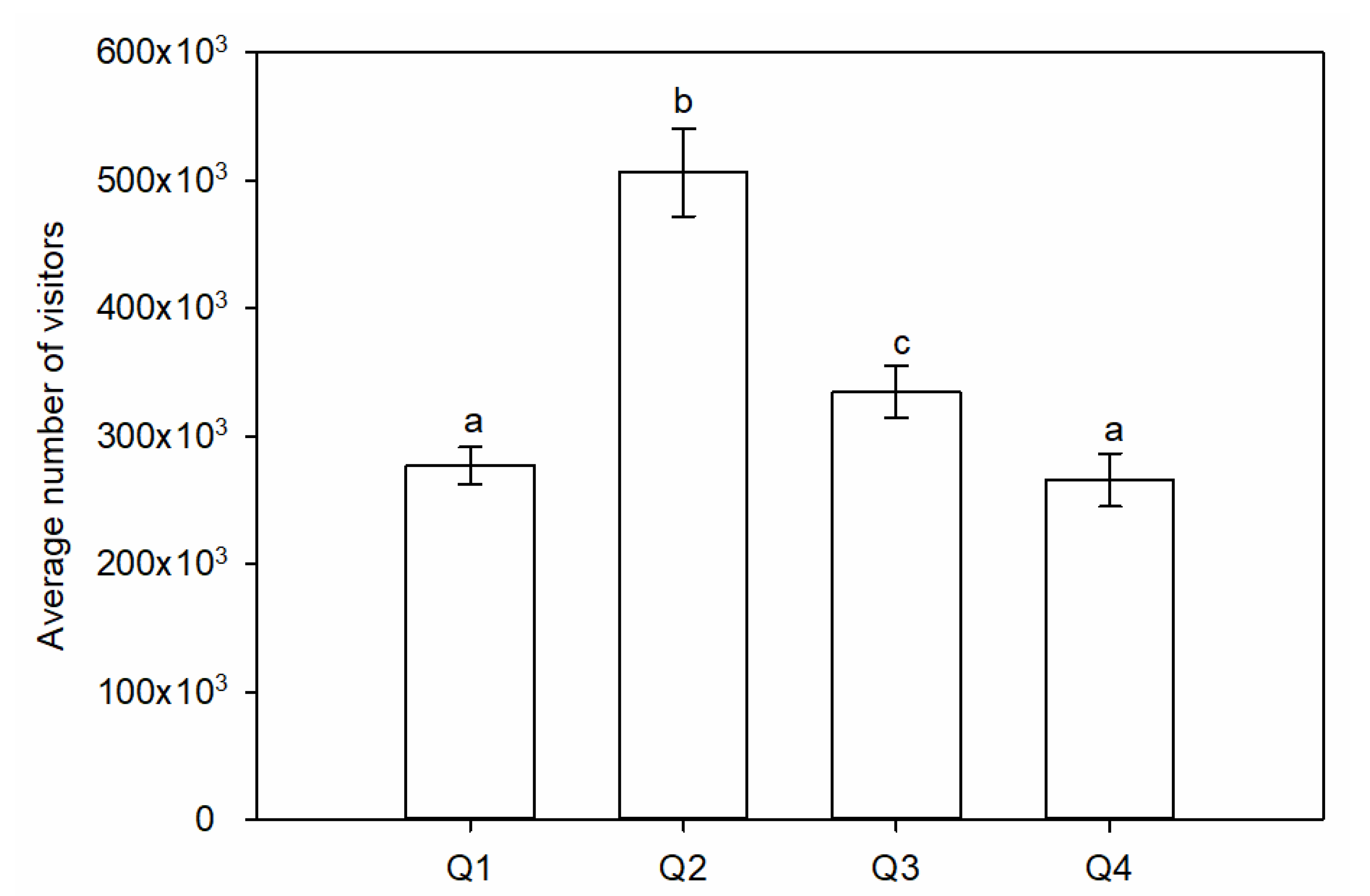
3. Results
4. Discussion
Supplementary Materials
Author Contributions
Funding
Institutional Review Board Statement
Informed Consent Statement
Data Availability Statement
Acknowledgments
Conflicts of Interest
References
- O’Riordan, T.; Sewell, W.D. Project Appraisal and Policy Review; John Wiley & Sons, Inc.: Hoboken, NJ, USA, 1981. [Google Scholar]
- Morgan, R.K. Environmental impact assessment: The state of the art. Impact Assess. Proj. Apprais. 2012, 30, 5–14. [Google Scholar] [CrossRef]
- Ramdani, M.; Elkhiati, N.; Flower, R.; Thompson, J.; Chouba, L.; Kraiem, M.; Ayache, F.; Ahmed, M. Environmental influences on the qualitative and quantitative composition of phytoplankton and zooplankton in North African coastal lagoons. Hydrobiologia 2009, 622, 113–131. [Google Scholar] [CrossRef]
- Parinet, B.; Lhote, A.; Legube, B. Principal component analysis: An appropriate tool for water quality evaluation and management—Application to a tropical lake system. Ecol. Model. 2004, 178, 295–311. [Google Scholar] [CrossRef]
- Vega, M.; Pardo, R.; Barrado, E.; Debán, L. Assessment of seasonal and polluting effects on the quality of river water by exploratory data analysis. Water Res. 1998, 32, 3581–3592. [Google Scholar] [CrossRef]
- Pugesek, B.H.; Tomer, A.; Von Eye, A. Structural Equation Modeling: Applications in Ecological and Evolutionary Biology; Cambridge University Press: Cambridge, UK, 2003. [Google Scholar]
- Arhonditsis, G.; Paerl, H.; Valdes-Weaver, L.; Stow, C.; Steinberg, L.; Reckhow, K. Application of Bayesian structural equation modeling for examining phytoplankton dynamics in the Neuse River Estuary (North Carolina, USA). Estuar. Coast. Shelf Sci. 2007, 72, 63–80. [Google Scholar] [CrossRef]
- Chou, W.R.; Fang, L.S.; Wang, W.H.; Tew, K.S. Environmental influence on coastal phytoplankton and zooplankton diversity: A multivariate statistical model analysis. Environ. Monit. Assess. 2012, 184, 5679–5688. [Google Scholar] [CrossRef]
- Sinotech. Environmental Impact Assessment—Development Plan of National Museum of Marine Biology & Aquarium; Environmental Protection Agency: Taipei City, Taiwan, 1992. (In Chinese) [Google Scholar]
- NSYSU. Environmental Impact Comparative Analysis Report—The Second Period of Development in National Museum of Marine Biology & Aquarium; Environmental Protection Agency: Beijing, China, 2007. (In Chinese) [Google Scholar]
- Tew, K.S.; Chen, H.L.; Han, C.C. Variation in reproductive traits of the river prawn, Macrobrachium nipponense (De Haan, 1849) (Caridea, Palaemonidae) among different sites in southern Taiwan. Crustaceana 2021, 94, 431–446. [Google Scholar] [CrossRef]
- Hsieh, W.C.; Lee, H.J.; Tew, K.S.; Lin, C.; Fan, K.S.; Meng, P.J. Estimating nutrient budgets in a coastal lagoon. Chin. Sci. Bull. 2010, 55, 484–492. [Google Scholar] [CrossRef]
- Tew, K.S.; Jhange, Y.S.; Meng, P.J.; Leu, M.Y. Environmental factors influencing the proliferation of microscopic epiphytic algae on giant kelp under aquarium conditions. J. Appl. Phycol. 2017, 29, 2877–2886. [Google Scholar] [CrossRef]
- Pai, S.C.; Riley, J.P. Determination of nitrate in the presence of nitrite in natural waters by flow injection analysis with a non-quantitative on-line cadmium redactor. Int. J. Environ. Anal. Chem. 1994, 57, 263–277. [Google Scholar] [CrossRef]
- Pai, S.C.; Tsau, Y.J.; Yang, T.I. pH and buffering capacity problems involved in the determination of ammonia in saline water using the indophenol blue spectrophotometric method. Anal. Chim. Acta 2001, 434, 209–216. [Google Scholar] [CrossRef]
- Pai, S.C.; Yang, C.C.; Riley, J.P. Effects of acidity and molybdate concentration on the kinetics of the formation of the phosphoantimonylmolybdenum blue complex. Anal. Chim. Acta 1990, 229, 115–120. [Google Scholar]
- Armstrong, F.A.J. The determination of silicate in sea water. J. Mar. Biol. Assoc. UK 1951, 30, 149–160. [Google Scholar] [CrossRef] [Green Version]
- Tew, K.S.; Meng, P.J.; Leu, M.Y. Factors correlating with deterioration of giant kelp Macrocystis pyrifera (Laminariales, Heterokontophyta) in an aquarium setting. J. Appl. Phycol. 2012, 24, 1269–1277. [Google Scholar] [CrossRef]
- Tew, K.S.; Lo, W.T. Distribution of Thaliacea in SW Taiwan coastal water in 1997, with special reference to Doliolum denticulatum, Thalia democratica and T. orientalis. Mar. Ecol. Prog. Ser. 2005, 292, 181–193. [Google Scholar] [CrossRef]
- Shannon, C.E.; Weaver, W. The Mathematical Theory of Communication; University of Illinois Press: Champaign, IL, USA, 1949. [Google Scholar]
- Howell, R.D. LISREL 8 with PRELIS2 for Windows. J. Mark. Res. 1996, 33, 377–381. [Google Scholar] [CrossRef]
- Malaeb, Z.A.; Summers, J.K.; Pugesek, B.H. Using structural equation modeling to investigate relationships among ecological variables. Environ. Ecol. Stat. 2000, 7, 93–111. [Google Scholar] [CrossRef]
- Schumacker, R.E.; Lomax, R.G. A Beginner’s Guide to Structural Equation Modeling, 2nd ed.; Lawrence Erlbaum Associates, Inc.: Mahwah, NJ, USA, 2004. [Google Scholar]
- Hoelter, J.W. The analysis of covariance structures: Goodness-of-fit indices. Sociol. Methods Res. 1983, 11, 325–344. [Google Scholar] [CrossRef]
- Finlay, K.; Beisner, B.E.; Patoine, A.; Pinel-Alloul, B. Regional ecosystem variability drives the relative importance of bottom-up and top-down factors for zooplankton size spectra. Can. J. Fish. Aquat. Sci. 2007, 64, 516–529. [Google Scholar] [CrossRef] [Green Version]
- Tew, K.S.; Kuo, J.; Cheng, J.O.; Ko, F.C.; Meng, P.J.; Mayfield, A.B.; Liu, P.J. Impacts of seagrass on benthic microalgae and phytoplankton communities in an experimentally warmed coral reef mesocosm. Front. Mar. Sci. 2021, 8, 680. [Google Scholar] [CrossRef]
- Tew, K.S.; Meng, P.J.; Lin, H.S.; Chen, J.H.; Leu, M.Y. Experimental evaluation of inorganic fertilization in larval giant grouper (Epinephelus lanceolatus Bloch) production. Aquac. Res. 2013, 44, 439–450. [Google Scholar] [CrossRef]
- Passow, U. Transparent exopolymer particles (TEP) in aquatic environments. Prog. Oceanogr. 2002, 55, 287–333. [Google Scholar] [CrossRef] [Green Version]
- Azetsu-Scott, K.; Passow, U. Ascending marine particles: Significance of transparent exopolymer particles (TEP) in the upper ocean. Limnol. Oceanogr. 2004, 49, 741–748. [Google Scholar] [CrossRef] [Green Version]
- Ortega-Retuerta, E.; Sala, M.M.; Borrull, E.; Mestre, M.; Aparicio, F.L.; Gallisai, R.; Antequera, C.; Marrasé, C.; Peters, F.; Simó, R.; et al. Horizontal and vertical distributions of transparent exopolymer particles (TEP) in the NW Mediterranean Sea are linked to chlorophyll a and O2 variability. Front. Microbiol. 2017, 7, 2159. [Google Scholar] [CrossRef] [Green Version]
- Zhou, Y.; Yu, D.; Yang, Q.; Pan, S.; Gai, Y.; Cheng, W.; Liu, X.; Tang, S. Variations of water transparency and impact factors in the Bohai and Yellow Seas from satellite observations. Remote Sens. 2021, 13, 514. [Google Scholar] [CrossRef]
- Liu, B.; de Swart, H.E.; de Jonge, V.N. Phytoplankton bloom dynamics in turbid, well-mixed estuaries: A model study. Estuar. Coast. Shelf Sci. 2018, 211, 137–151. [Google Scholar] [CrossRef]
- Chang, Y.W.; Chern, J.S. A preliminary study on the potential spaceports for suborbital space tourism and intercontinental point-to-point transportation in Taiwan. Acta Astronaut. 2021, 181, 492–502. [Google Scholar] [CrossRef]
- Kang, Y.; Kang, Y.-H.; Kim, J.-K.; Kang, H.Y.; Kang, C.-K. Year-to-year variation in phytoplankton biomass in an anthropogenically polluted and complex estuary: A novel paradigm for river discharge influence. Mar. Pollut. Bull. 2020, 161, 111756. [Google Scholar] [CrossRef]
- Kang, Y.; Moon, C.H.; Kim, H.J.; Yoon, Y.H.; Kang, C.K. Water quality improvement shifts the dominant phytoplankton group from cryptophytes to diatoms in a coastal ecosystem. Front. Mar. Sci. 2021, 8, 1125. [Google Scholar] [CrossRef]
- Yamamichi, M.; Kazama, T.; Tokita, K.; Katano, I.; Doi, H.; Yoshida, T.; Hairston, N.G.; Urabe, J. A shady phytoplankton paradox: When phytoplankton increases under low light. Proc. R. Soc. B Biol. Sci. 2018, 285, 20181067. [Google Scholar] [CrossRef]
- Antell, G.S.; Saupe, E.E. Bottom-up controls, ecological revolutions and diversification in the oceans through time. Curr. Biol. 2021, 31, R1237–R1251. [Google Scholar] [CrossRef]
- Silva, L.H.S.; Huszar, V.L.M.; Marinho, M.M.; Rangel, L.M.; Brasil, J.; Domingues, C.D.; Branco, C.C.; Roland, F. Drivers of phytoplankton, bacterioplankton, and zooplankton carbon biomass in tropical hydroelectric reservoirs. Limnologica 2014, 48, 1–10. [Google Scholar] [CrossRef]
- Hoang, H.T.T.; Duong, T.T.; Nguyen, K.T.; Le, Q.T.P.; Luu, M.T.N.; Trinh, D.A.; Le, A.H.; Ho, C.T.; Dang, K.D.; Némery, J.; et al. Impact of anthropogenic activities on water quality and plankton communities in the Day River (Red River Delta, Vietnam). Environ. Monit. Assess. 2018, 190, 67. [Google Scholar] [CrossRef]


| Range | Mean ± SD | |
|---|---|---|
| Temperature (°C) | 24.1–31.6 | 27.8 ± 2.1 |
| Salinity | 18.8–34.6 | 32.9 ± 1.8 |
| Dissolved oxygen (mg L−1) | 4.7–10.0 | 6.7 ± 0.7 |
| pH | 7.87–8.40 | 8.18 ± 0.11 |
| Transparency (m) | 1.0–20.0 | 8.1 ± 4.4 |
| Turbidity (ntu) | 0.20–16.4 | 0.90 ± 2.02 |
| Suspended solids (mg L−1) | 1.84–16.70 | 6.55 ± 3.25 |
| NO3-N (mg L−1) | 0.001–0.193 | 0.024 ± 0.033 |
| NH3-N (mg L−1) | 0.001–0.289 | 0.018 ± 0.042 |
| PO4-P (mg L−1) | 0.002–0.008 | 0.004 ± 0.002 |
| SiO2-Si (mg L−1) | 0.020–1.382 | 0.121 ± 0.217 |
| Chl a (µg L−1) | 0.02–2.53 | 0.33 ± 0.50 |
| Phytoplankton density (cell L−1) | 260–180,400 | 27,537 ± 36,921 |
| Phytoplankton species number | 4–23 | 13 ± 4 |
| Phytoplankton Shannon–Weaver diversity index | 0.17–2.53 | 1.57 ± 0.50 |
| Zooplankton density (ind 100 m−3) | 299–93,231 | 12,826 ± 20,171 |
| Zooplankton class number | 9–25 | 19 ± 4 |
| Zooplankton Shannon–Weaver diversity index | 0.62–2.30 | 1.60 ± 0.35 |
| Variable | PC 1 | PC 2 | PC 3 |
|---|---|---|---|
| Transparency | −0.277 | −0.639 | −0.057 |
| Temperature | 0.211 | 0.311 | −0.472 |
| Salinity | −0.822 | −0.090 | 0.358 |
| NO3-N | 0.763 | 0.226 | 0.122 |
| PO4-P | 0.186 | 0.012 | 0.094 |
| SiO2-Si | 0.916 | 0.141 | 0.071 |
| NH3-N | 0.800 | 0.195 | 0.174 |
| Turbidity | 0.683 | 0.092 | −0.412 |
| Chl a | −0.024 | 0.728 | −0.083 |
| Suspended solids | 0.180 | 0.643 | −0.143 |
| Eigenvalues | 3.393 | 1.574 | 1.401 |
| Total variance (%) | 33.94 | 15.74 | 14.01 |
| (A) PC1 | |||||
| Two-way ANOVA | Multiple Comparison | ||||
| DF | F | p | |||
| Season | 3 | 3.76 | 0.014 * | Q3 a Q2 a Q1 ab Q4 b | |
| Station | 5 | 3.91 | 0.003 * | S1 a S10 b S4 b S7 b S11 b S2 b | |
| Season × Station | 15 | 1.39 | 0.175 | ||
| (B) PC2 | |||||
| Two-way ANOVA | Multiple Comparison | ||||
| DF | F | p | |||
| Season | 3 | 7.98 | <0.001 * | Q2 a Q4 a Q3 a Q1 b | |
| Station | 5 | 1.36 | 0.252 | ||
| Season × Station | 15 | 0.27 | 0.996 | ||
| (C) PC3 | |||||
| Two-way ANOVA | Multiple Comparison | ||||
| DF | F | p | |||
| Season | 3 | 12.77 | <0.001 * | Q1 a Q4 b Q3 bc Q2 c | |
| Station | 5 | 0.72 | 0.611 | ||
| Season × Station | 15 | 0.70 | 0.778 | ||
Publisher’s Note: MDPI stays neutral with regard to jurisdictional claims in published maps and institutional affiliations. |
© 2022 by the authors. Licensee MDPI, Basel, Switzerland. This article is an open access article distributed under the terms and conditions of the Creative Commons Attribution (CC BY) license (https://creativecommons.org/licenses/by/4.0/).
Share and Cite
Chou, W.-R.; Hsieh, H.-Y.; Hong, G.-K.; Ko, F.-C.; Meng, P.-J.; Tew, K.S. Verification of an Environmental Impact Assessment Using a Multivariate Statistical Model. J. Mar. Sci. Eng. 2022, 10, 1023. https://doi.org/10.3390/jmse10081023
Chou W-R, Hsieh H-Y, Hong G-K, Ko F-C, Meng P-J, Tew KS. Verification of an Environmental Impact Assessment Using a Multivariate Statistical Model. Journal of Marine Science and Engineering. 2022; 10(8):1023. https://doi.org/10.3390/jmse10081023
Chicago/Turabian StyleChou, Wei-Rung, Hung-Yen Hsieh, Guo-Kai Hong, Fung-Chi Ko, Pei-Jie Meng, and Kwee Siong Tew. 2022. "Verification of an Environmental Impact Assessment Using a Multivariate Statistical Model" Journal of Marine Science and Engineering 10, no. 8: 1023. https://doi.org/10.3390/jmse10081023
APA StyleChou, W.-R., Hsieh, H.-Y., Hong, G.-K., Ko, F.-C., Meng, P.-J., & Tew, K. S. (2022). Verification of an Environmental Impact Assessment Using a Multivariate Statistical Model. Journal of Marine Science and Engineering, 10(8), 1023. https://doi.org/10.3390/jmse10081023