Next Article in Journal
Research of Intelligent Logistics and High-Quality Economy Development for Yangtze River Cold Chain Shipping Based on Carbon Neutrality
Previous Article in Journal
Dynamic Analysis on Pile Group Supported Offshore Wind Turbine under Wind and Wave Load
 
 
Correction published on 21 October 2022, see J. Mar. Sci. Eng. 2022, 10(10), 1560.
Article

Advancing Three-Dimensional Coupled Water Quality Model of Marine Ranches: Model Development, Global Sensitivity Analysis, and Optimization Based on Observation System

1
First Institute of Oceanography, and Key Laboratory of Marine Science and Numerical Modeling, Ministry of Natural Resources, Qingdao 266061, China
2
Laboratory for Regional Oceanography and Numerical Modeling, Pilot National Laboratory for Marine Science and Technology, Qingdao 266237, China
3
Shandong Key Laboratory of Marine Science and Numerical Modeling, Qingdao 266061, China
4
North China Sea Marine Forecasting Center of SOA, Qingdao 266061, China
5
Physical Oceanography Laboratory/CIMST, Ocean University of China and Qingdao National Laboratory for Marine Science and Technology, Qingdao 266100, China
*
Author to whom correspondence should be addressed.
J. Mar. Sci. Eng. 2022, 10(8), 1028; https://doi.org/10.3390/jmse10081028
Submission received: 2 May 2022 / Revised: 20 July 2022 / Accepted: 20 July 2022 / Published: 27 July 2022 / Corrected: 21 October 2022
(This article belongs to the Section Physical Oceanography)

Abstract

:
Marine ranching is a stock enhancement project that has been an important part of aquaculture in China. Due to the lack of scientific management, disasters have occurred, resulting in millions of economic losses. Based on the observation system of marine ranches, a three-dimensional water quality model of marine ranches was developed to study the spatio-temporal variation of key ecological indicators, including the concentrations of chlorophyll-a, zooplankton, detritus, nutrients, and dissolved oxygen (DO). The model is coupled offline with the residual current, temperature, and salinity simulated by a regional oceanic modeling system (ROMS). The conservative characteristic finite difference (C-CFD) scheme is introduced to solve the equations, which guarantees model stability and mass conservation and allows for a larger time step compared to traditional difference schemes. In state-of-the-art water quality models, the biogeochemical processes are parameterized. Due to the complexity of the water quality model, a combination of global sensitivity analysis (GSA) and the adjoint method is introduced as the methodology to optimize the model parameters. Morris’ sampling method is implemented as the GSA method to find out the key factors of the water quality model. The optimization of sensitive parameters with the adjoint method significantly improves the model precision, while the other parameters can be set as empirical values. The results indicate that the combination of GSA and the adjoint method is efficient in the parameter optimization of the water quality model. The model is applicable in marine ranches.

1. Introduction

Marine ranching has been an important part of aquaculture in China [1,2]. Marine ranching is an artificial ecosystem; however, due to the lack of scientific management, it is difficult to detect the potential ecological risks of marine ranches in time. Disasters have occurred, resulting in millions of economic losses. With the development of observation systems in marine ranches, a three-dimensional water quality model with optimization that combines GSA and the adjoint method is essential for the sustainable development of marine ranches, to forecast and analyze the spatio-temporal variations of the environment.
Water quality modeling is an important methodology for studying the ecological dynamics of both rivers and seas [3,4]. Based on the observation system deployed in marine ranches, we were able to develop a water quality model of marine ranches. In state-of-the-art water quality models, the biogeochemical processes are parameterized. Due to the uncertainty of the model parameters, uncertainty exists in these models. Therefore, parameter optimization is essential for improving the simulation. However, the complex solution space of the parameter optimization places high demands on both the amount of observation data and the reliability of the optimization method, especially in complex models [5]. Determining the sensitive parameters and reducing the solution space is essential in parameter optimization. It was pointed out that a change made to one parameter could interact with another highly correlated one [6]. Several studies have expounded that the impact of parameters with weak inter-correlations on models cannot be neglected [7,8]. According to the interactions among the parameters, the sensitivity analysis methods can be divided into two types: local sensitivity analysis (LSA) and GSA [9]. GSA is a kind of sensitivity analysis method that tests the impacts of multiple parameters simultaneously and is able to capture the interactions among the parameters, while LSA analyzes the parameters one by one. In this paper, Morris’ sampling method [10] is implemented as the GSA method due to its high efficiency. In this study, we only optimized the sensitive parameters and kept the insensitive parameters as the empirical values to reduce computation.
Model parameter optimization is the methodology that assimilates observations and optimizes the model parameters to improve the model precision. Among the assimilation methods, 4D-Var has been proven to be one of the most effective and powerful approaches in ecological models [5,11,12,13] and is able to optimize the parameters and improve the simulation precision simultaneously.
This paper is organized as follows: the methods, model settings, and data description are introduced in Section 2; the GSA and parameter optimization results and discussions are presented in Section 3; the conclusions are presented in Section 4.

2. Methods

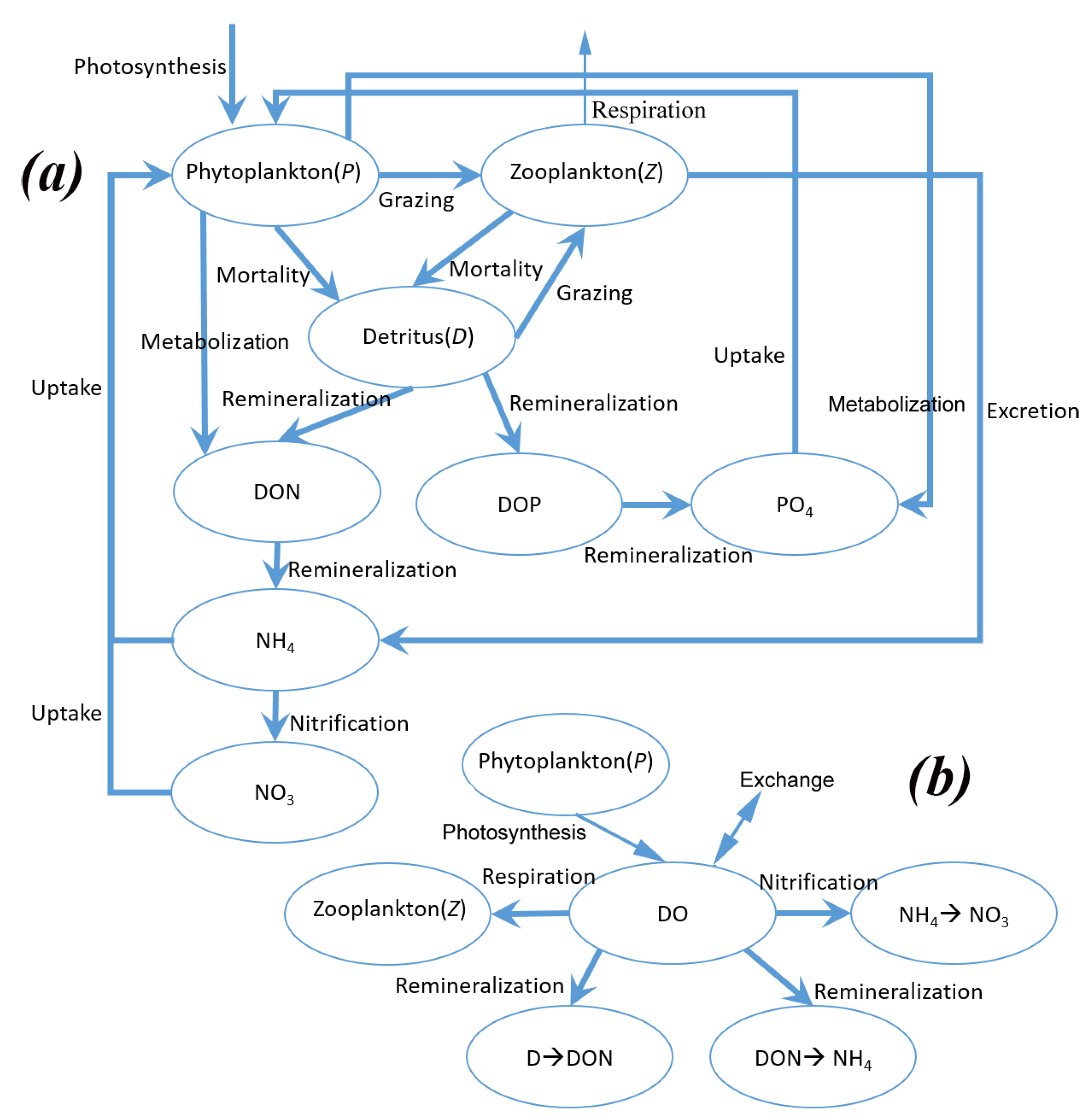
2.1. Water Quality Model

Based on previous studies of water quality models [4,14,15], an offline-coupled three-dimensional hydrodynamic water quality model was developed. This model is different from the previous models in the following ways: although the water quality model is a nitrogen-based model (which means all the state variables except DO are calculated using the unit mmol N/l), the phosphate and dissolved organic phosphorus (DOP) are taken into consideration. In addition, the nitrification process and the state variable DO are included. The state variables of this model include phytoplankton, zooplankton, detritus, dissolved organic nitrogen (DON), DOP, phosphate (PO4), ammonium (NH4), nitrate (NO3), and DO. The schematic structure of the water quality model is presented in Figure 1.
In the water quality model, the phytoplankton growth rate is described as a function that depends on the water temperature, nutrient limitation, and photosynthetically active irradiance. The temperature effect on phytoplankton growth is described as an exponential function [15,16], and the light control of photosynthesis is described as Steele’s function [17]. Michaelis–Menten functions are used to describe the nutrient limitation [14,18]. The phytoplankton biomass budget includes the photosynthesis process, mortality, grazing by zooplankton, and metabolization. The metabolization process includes respiration and exudation and is parameterized as a function related to the phytoplankton growth rate. More details about the model parameters and governing equations can be found in Table 1 and the Appendix A.
Regarding the budget of the DO concentration, the dissolved oxygen is mainly supplied by the photosynthesis process and exchanged at the sea surface. The respiration process of phytoplankton and zooplankton, nitrification, remineralization, and exchange with sediment all consume oxygen.
To improve the calculation efficiency of the water quality model, the conservative characteristic finite difference (C-CFD) scheme was introduced as the difference scheme of this model for numeric calculation [19,20]. The C-CFD scheme guarantees model stability and mass conservation and allows for a larger time step compared to traditional difference schemes. More details about the C-CFD scheme can be found in the Appendix B.

2.2. Global Sensitivity Analysis

Based on the Morris sampling method, the frame of global sensitivity analysis was established. The process can be generalized into three steps—discretization, sampling, and sensitivity analysis. The discretization method is used to normalize and discretize each parameter into the same range. Then the sampling method is implemented to choose the parameter randomly. According to the randomly chosen parameter, the elemental effect (EE) is calculated and the process is continuously repeated until the mean value of EE is convergent. The global sensitivity is defined as the mean value of EE.

2.2.1. Discretization

Firstly, the range of each parameter is normalized into a range of [0, 1]. Then, the parameters are discretized into { 0 ,   1 p 1 ,   2 p 1 , , 1 } . The simulation results of the water quality model are denoted as a function, y = y ( x 1 , x 2 , x m ) , where x 1 , x 2 , x m represents the parameters, and m is the number of parameters. The EE of a certain parameter xi is defined as shown in Equation (1):
E E i = | [ y ( x 1 , x 2 , , x i 1 , x i + δ , x i + 1 , , x m ) y ( x ) ] / δ |
δ = m p 1 , m = 1 , 2 , , p 1

2.2.2. Sampling

According to Morris’ sampling method, δ is random. Each time a random parameter is chosen, the EE is calculated. The process is repeated until the EE of each parameter is calculated and the mean value of EE is convergent. To achieve this goal, a sampling method is required.
A k-dimensional random vector x* is defined, for which all the elements are randomly chosen from { 0 ,   1 p 1 ,   2 p 1 , , 1 } .
A (k + 1) × k dimensional down triangle matrix B is defined as follows:
B = ( 0 0 0   0   1 0 0   0   1 1 0   0 1 1 1   0         1 1 1   1 )
A k-dimensional diagonal matrix D* is defined, of which all the elements are randomly set as −1 or 1. A (k + 1)-dimensional vector Jk + 1,1 is defined, of which all the elements are 1.
A (k + 1) × k dimensional matrix J* is defined as follows:
J = [ ( 2 B J ) D + J ] / 2
Then, the sampling matrix B* is defined as follows:
B = ( J k + 1 , 1 x + δ J ) P
From the matrices given above, it can be deduced that B* obtains its value randomly. In every two adjacent rows of B*, there is only one different parameter.

2.2.3. Elemental Effect

Considering the two adjacent rows of B*:
B ( j ) = ( x 1   x j 1   x m x 1 x j 2   x m )
x j 1 x j 2 = δ
Taking B ( j ) as the parameters of the water quality model, the EE of parameter j is shown as follows:
E E j = y ( x 1 , x 2 , , x j 1 , x m ) y ( x 1 , x 2 , , x j 2 , x m ) δ y ( x 1 , x 2 , , x j 2 , x m )
where the function y ( x 1 , x 2 , , x j , x m ) represents the model output. The process is repeated until the EE of each parameter is calculated and the mean value of EE is convergent. Then, the mean value of the elemental effect is defined as sensitivity and the standard deviation is defined as the correlation between each parameter.

2.3. Parameter Optimization

The parameter optimization method used in this water quality model is the 4D-var method, of which the flowchart is shown in Figure 2. To start the optimization process, the parameters are initialized with prior values. Then the water quality model is run, which is also denoted as the forward model. The simulation results of the state variables are used to calculate the cost function. If the value of the cost function is lower than the criterion, the optimization is terminated; otherwise, the adjoint model is run to adjust the model parameters, and the water quality model is recalculated until the value of the cost function is lower than the criterion.
The cost function is defined as follows:
J = 1 2   [ K ( P P ¯ ) 2 ]
where P represents the simulated concentration of phytoplankton, and P ¯ represents the observed concentration of phytoplankton. K is the weighting matrix. The elements of the weighting matrix are 1 where the observation of the corresponding grid point is available, and 0 otherwise. The cost function serves as an indicator of the model precision. To optimize the parameters and assimilate the water quality model, the cost function should be minimized. Therefore, the optimization problem is defined as follows:
min : J ( x )
where J ( x ) is already defined in Equation (9) and x represents the parameters to be optimized. ‘min’ represents the minimum value [5]. The Lagrangian multiplier method is introduced [5] to calculate the gradient. The Lagrangian function is defined as follows:
L = J + Ω [ P G ( P ) ] d Ω
where Ω denotes the model domain; P represents the adjoint variable of P, and G(P) represents the Equation (B1). More details about the equations can be found in Appendix B.
According to the Lagrangian multiplier method, the first-order derivative of Equation (11), with respect to the state variables P and parameters, should be zero. Taking the parameter kPPT_G and Iopt as examples, the equations are shown as follows:
L P = 0 ,   L k P P T _ G = 0 ,   L I o p t = 0
By solving the equations above, the gradient of the parameters can be determined. The dimensions of the parameters and gradient vector of the cost function are denoted as N and J ( x i k ) , respectively, with respect to the i-th control variable ( 1 i N ) at the k-th iteration step. The following iteration is expressed to solve Equation (10):
x i k + 1 = x i k + α k d k ,   k = 1 , 2
where dk represents the gradient of xk, and αk represents the adjustment coefficient, which satisfies the strong Wolfe conditions [21,22]. The αk in Equation (13) is defined as shown in Equations (14) and (15):
( x i k + α k d k ) J ( x i k ) c 1 α k ( d k ) T ( d k )
| J ( x i k + α k d k ) T d k | c 2 | ( d k ) T d k |
where 0 < c1 < c2, and T denotes the matrix transposition.
Then, the steepest descent method is implemented to adjust the parameters, and it is expressed as follows:
d k = J ( x i k )
With Equation (16), Equation (13) can be solved. Then, the optimization problem in Equation (10) can be solved.

2.4. Numerical Experiment Design

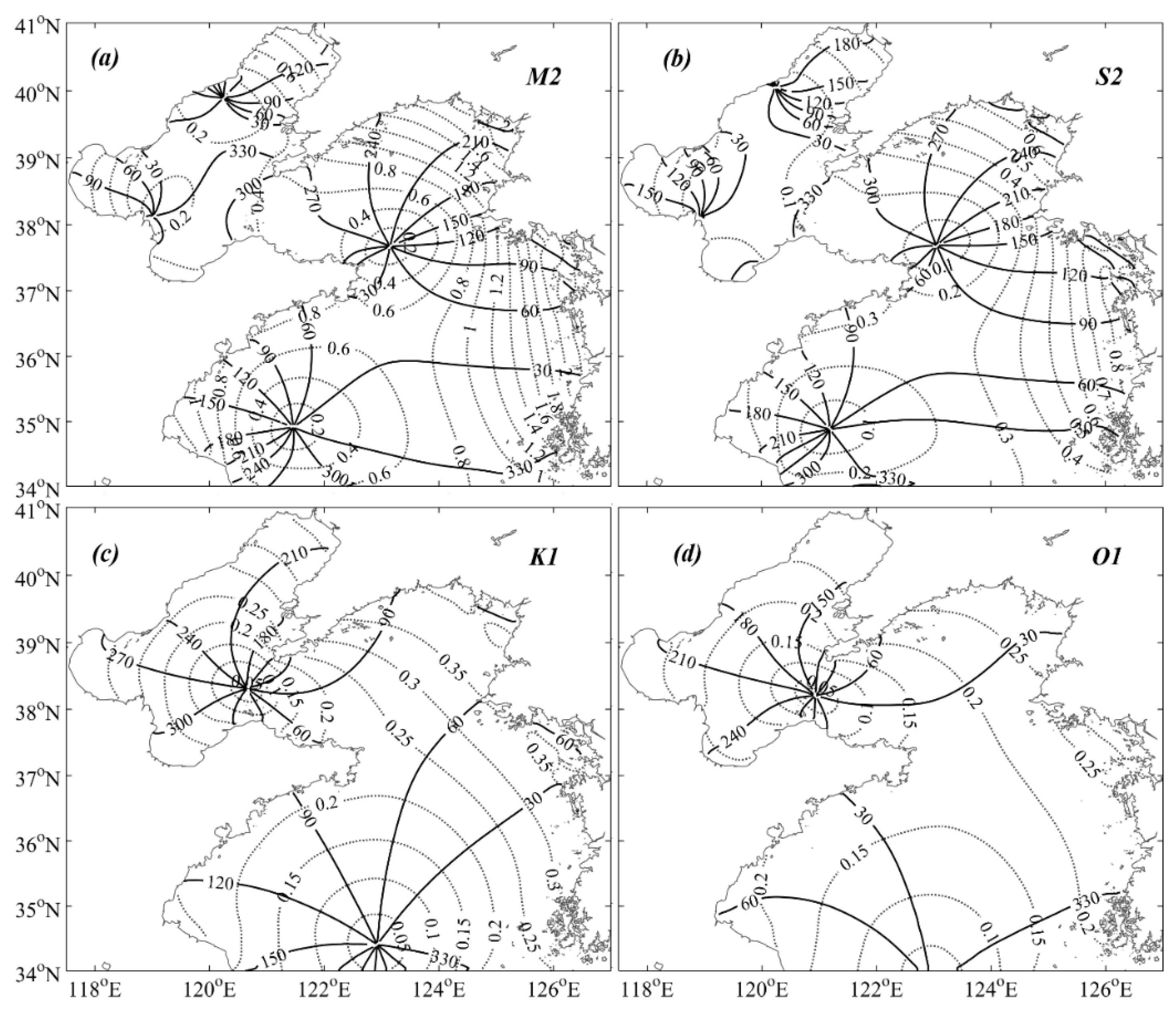
2.4.1. Model Settings

The hydrodynamic background is calculated by the three-dimensional regional ocean modeling system (ROMS) [23]. The study site was the Bohai Sea and the Yellow Sea, as shown in Figure 3 (117.5° E–127° E, 34° N–41° N). Horizontal orthogonal grids were applied to calculate the model domain, with a resolution of 3’ × 3’. The time step was set as 20 s. There were 6 uniform layers in the vertical direction. The surface atmospheric forcing fields and shortwave radiation were derived from the Comprehensive Ocean-Atmosphere Data Set (COADS) [24]. The salinity and temperature were obtained from the climatological dataset of the World Ocean Atlas 2013 (WOA13; available online at https://www.nodc.noaa.gov/OC5/woa13, accessed on 1 January 2017). The open boundary was set at 34°N. The sea surface height variations induced by astronomical tides at the open boundary were calculated with the tidal harmonic constants of four dominating tidal constituents, including M2, S2, K1, and O1, which were obtained from Oregon State University Tidal Inversion Software [25]. The simulation of ROMS started one year before the simulation of the water quality model to make the simulated background forcing stable enough for the water quality model. The ROMS started on 1 January 2015 and terminated on 31 December 2016. The calculated sea surface height, residual current, temperature, and salinity were exported as the background forcing for the water quality model with a time range from 1 January 2016 to 31 December 2016.
The sea surface height calculated by the ROMS in the time range from 1 January 2016 to 31 December 2016 was processed using harmonic analysis to extract the tidal constitutes. The cotidal chart is shown in Figure 4 and is consistent with previous studies on tidal models [26,27,28,29]. Then, the water quality model was coupled offline with the hydrodynamic field.
The horizontal grid and vertical layers of the water quality model are consistent with the hydrodynamic model. With the help of the C-CFD scheme, the time step could be set as 1 h, and the scheme guaranteed model stability and mass conservation. The water quality model was run within the period from 1 January to 31 December 2016.

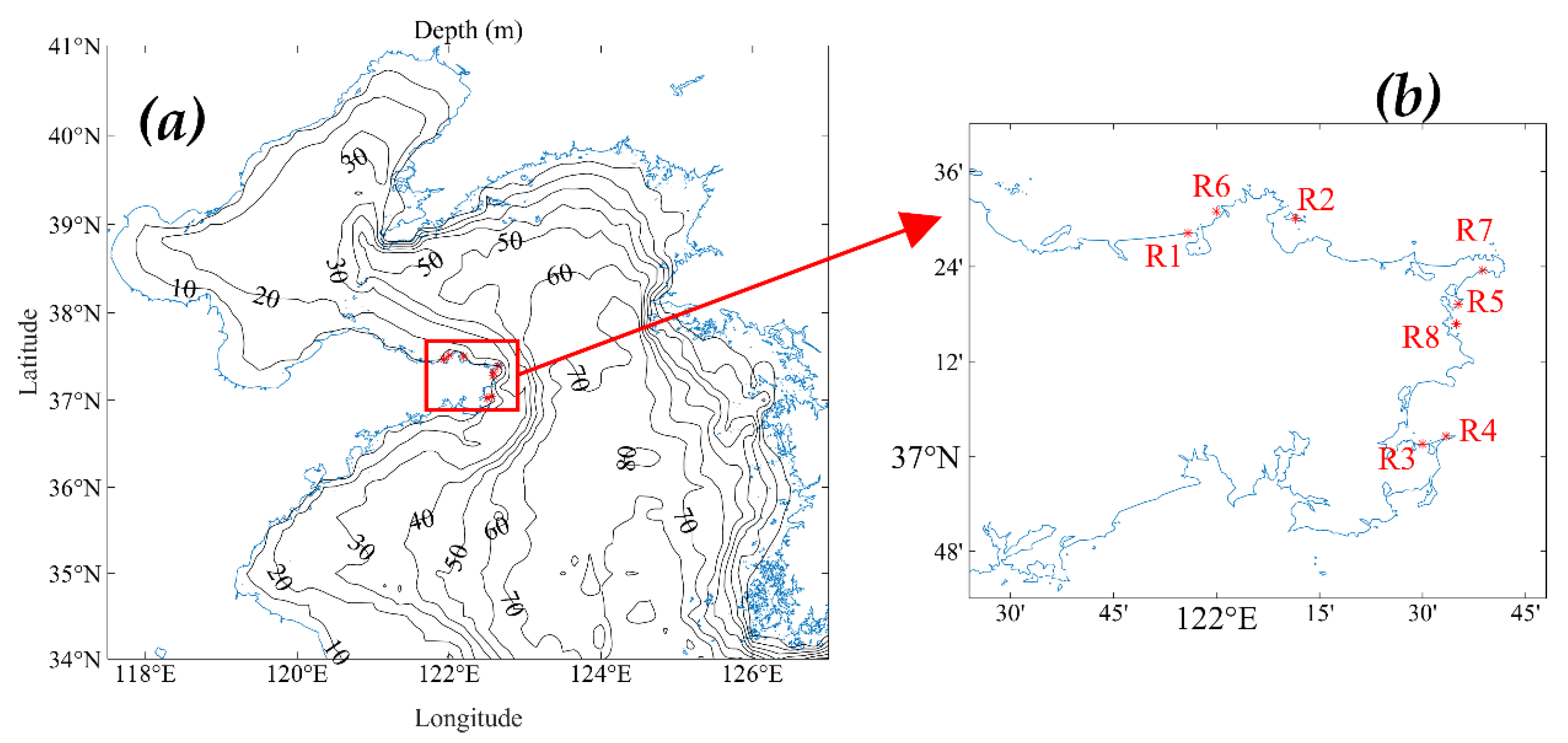
2.4.2. Data Descriptions

Daily observations of 8 marine ranches, including the chlorophyll-a concentration, water temperature, and salinity at full water depth, with a time range from May to August 2016, were obtained from the observation systems of marine ranches. The locations of the ranches are shown in Figure 3. The Pauta criterion was implemented to remove the spurious values of observations. The chlorophyll-a concentration was observed by SBE WQM, and the temperature and salinity were observed by SEB 63 CTD.
To initialize and calibrate the water quality model, we used the observed temperature, salinity, and open-source datasets to set the initial values of the model. The observed chlorophyll-a concentration was used to calibrate the simulated concentration of phytoplankton and optimize the model parameters.
The open-source datasets included the CSIRO Atlas of Regional Seas (CARS2009; available online at http://www.cmar.csiro.au/cars, accessed on 1 January 2017) and the Sea-Viewing Wide Field-of-View Sensor (SeaWIFS; available online at https://seawifs.gsfc.nasa.gov/, accessed on 1 January 2017). The chlorophyll-a concentration from SeaWIFS was used to set the initial background value of the phytoplankton concentration by the coefficient conversion [15]. The nitrate, phosphorus, and dissolved oxygen from CARS2009 were used to set the initial values of the corresponding state variables. The initial values of the other state variables were set as the empirical values from [15]. Before being applied to the water quality model, both datasets were interpolated into the model grid with the modified Cressman interpolation method described in [30].

3. Results and Discussion

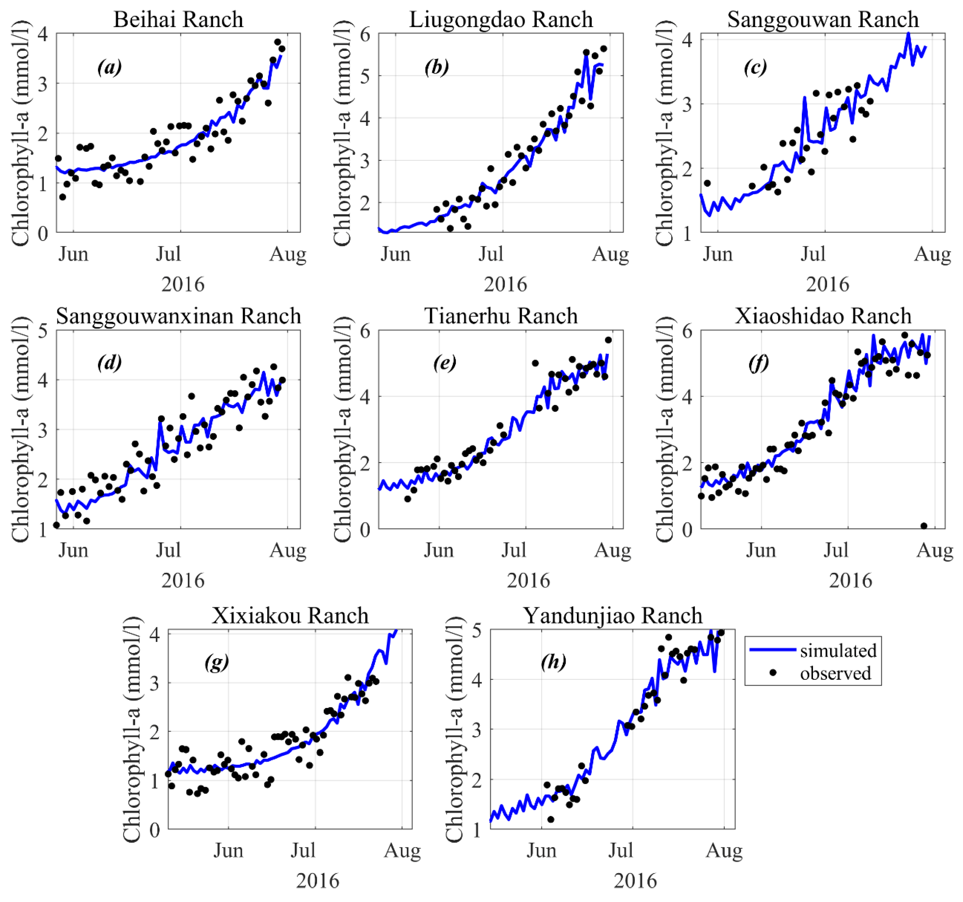
3.1. Simulation Results

The simulated phytoplankton concentration was converted to the chlorophyll-a concentration. As shown in Figure 5, with all the aforementioned observations of eight marine ranches, we compared and calibrated the simulation results and observations from June–August 2016. The water quality model captured an increasing trend of the chlorophyll-a concentration during the summer time, which agrees well with the observations. The mean square errors (MAEs) between the model results and observations are listed in Table 2.
To further improve the model, GSA and parameter optimization was implemented as follows:
(1)
GSA was applied to the parameters to determine the sensitive parameters and summarize their effects on different state variables;
(2)
The sensitive parameters were optimized and the effects of optimization on the model results were analyzed.
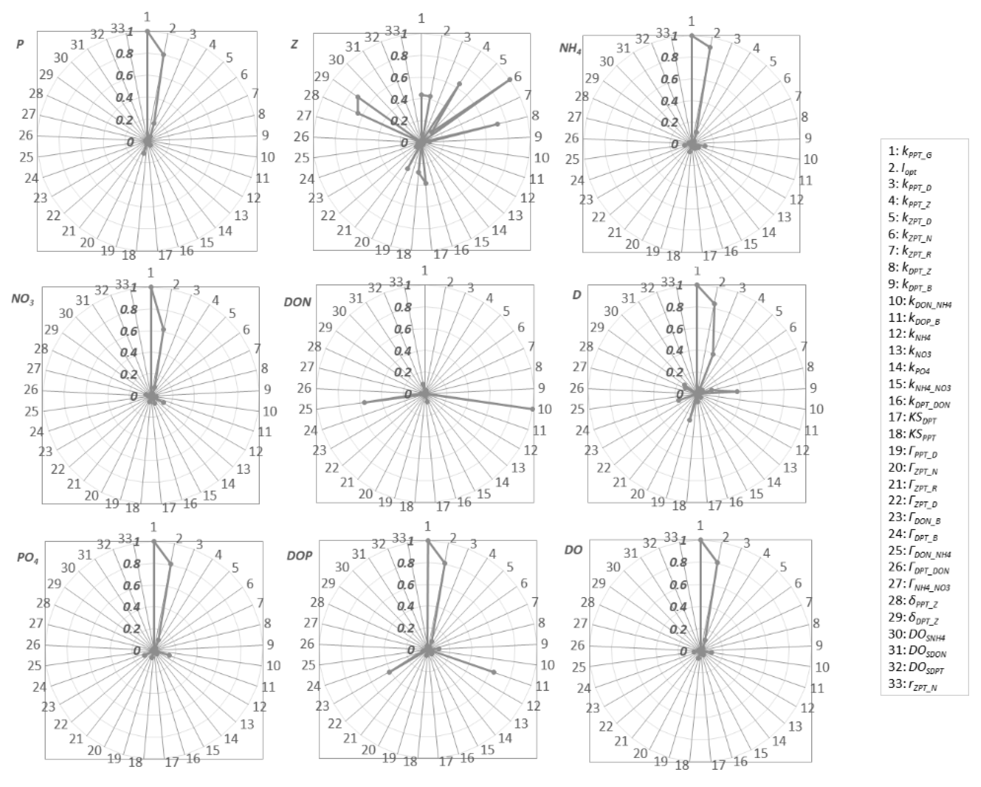
3.2. GSA Results

The EE was standardized to [0, 1] and ranked as shown in Figure 6. The sensitivity of different parameters and their impact on different state variables were different. The maximum phytoplankton growth rate (kPPT_G) and optimal light irradiance (Iopt) had a significant effect on the phytoplankton, ammonium, nitrate, detritus, phosphorus, DOP, and DO, as shown in Figure 6, because both parameters directly influenced the photosynthesis process, and thus, influenced the growth rate of phytoplankton, which indirectly influenced the nutrient uptake process and DO concentration. The zooplankton biomass was sensitive to kZPT_N (zooplankton excretion rate), kPPT_Z (zooplankton grazing rate on phytoplankton), kDPT_Z (zooplankton grazing rate on detritus), kDPT_Z (assimilation efficiency for phytoplankton), and δPPT_Z (assimilation efficiency for detritus) since all of these parameters influenced the grazing and excretion process of zooplankton. The DON concentration was sensitive to kDON_NN4 (remineralization rate of DON at 0 °C) and ГDON_NH4 (temperature coefficient for the remineralization of DON), which means that the remineralization process was a key factor for the DON concentration. To sum up, among all the parameters, kPPT_G and Iopt were the two most sensitive parameters.

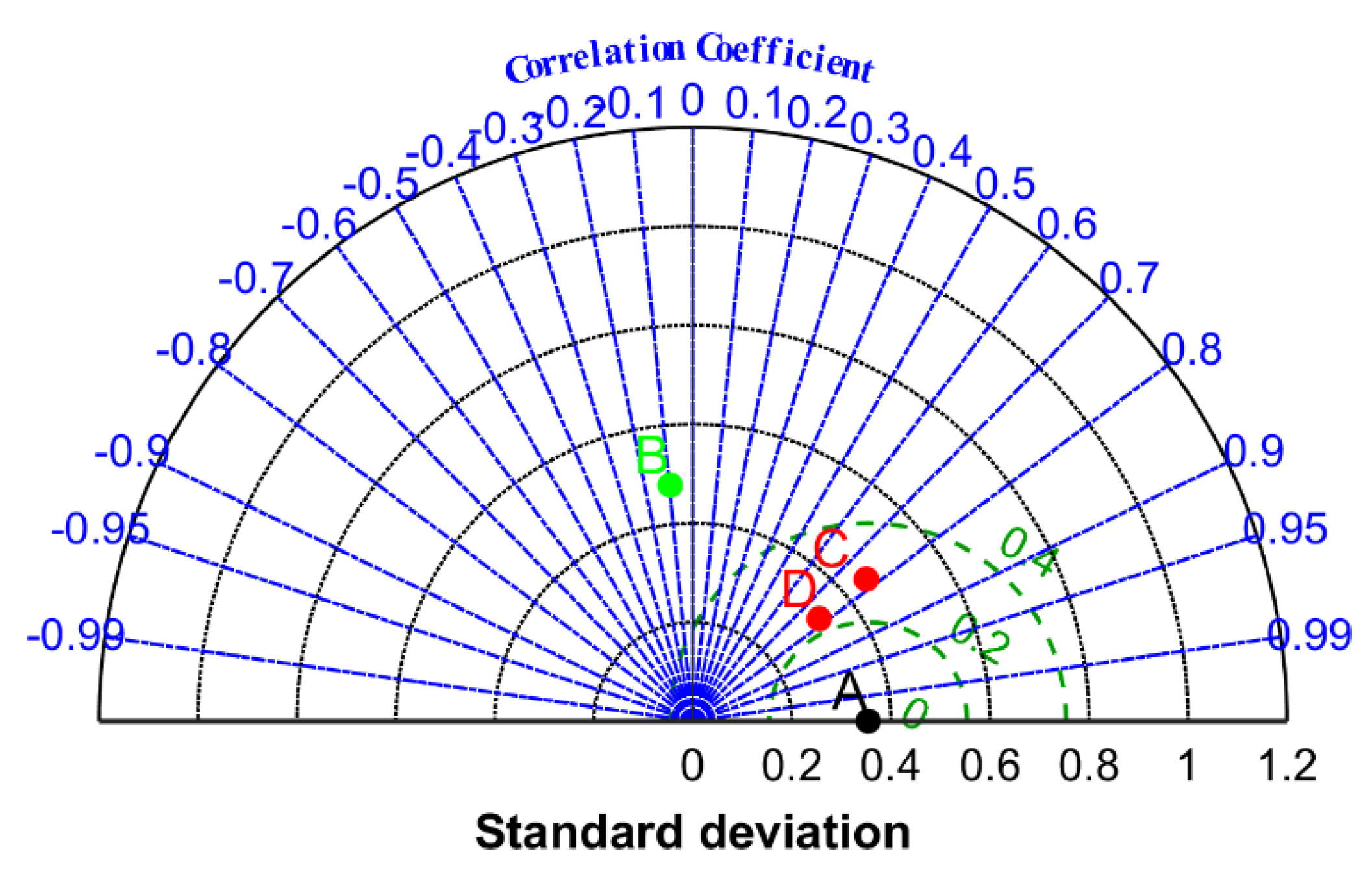
3.3. Parameter Optimization

Since most of the state variables were sensitive to kPPT_G and Iopt, we mainly optimized these two parameters. In the actual simulation, the spatial patterns of the parameters were unknown. Generally, all the parameters were set as the constant values listed in Appendix A. During the optimization, we treated the parameters as constant or spatially varying. Taking the joint parameter kPPT_G/Iopt as an example, three numerical experiments were implemented, including simulation without optimization, simulation with the optimization of constant parameters, and simulation with the optimization of spatially varying parameters. The results of the three numerical experiments, as well as the observed chlorophyll-a concentration, are shown in Figure 6. For further analysis of the change in the model precision, the normalized cost function versus the iterations is shown in Figure 7.
In Figure 8, the Taylor diagram shows that the simulation results with parameter optimization are closer to the observation than that without optimization. The results with the optimization of the spatially varying parameters are better than the constant ones, indicating that the spatial variations of parameters cannot be neglected in water quality modeling, while our method is capable of optimizing the spatially varying parameters. By optimizing the parameters, the correlation between the simulated and observation results improved from −0.1 to 0.8, and the deviation was significantly reduced. In Figure 7b, the cost function with the optimization of the spatially varying joint parameters is smaller than the other two and converges to 0.654.
As described in Section 3.1, the chlorophyll-a concentrations in different marine ranches kept increasing and reached their highest values in August, so in this section, the monthly mean chlorophyll-a concentration in August is shown in Figure 9. According to the spatial distribution of the chlorophyll-a concentration, the highest values of the chlorophyll-a concentration are mainly distributed in the three bays of the Bohai Sea, which matches the spatial distribution of pollutants in the Bohai Sea due to terrestrial discharge [5]. It was pointed out that phytoplankton increases during seasons in which nutrient loadings are high [15]. The high concentration of pollutants provides enough nutrients for the growth of phytoplankton. The chlorophyll-a concentrations in marine ranches are also higher than in adjacent regions.
With respect to the model results, it is possible to evaluate the environmental capacity around the regions of marine ranches and conduct reasonable management to avoid overstocking. The impact of marine ranches on coastal regions is nonnegligible. Compared to previous studies on marine ranching [31,32], we have taken a step towards systematic research on marine ranching.
Based on previous studies of water quality models [4,14,15], we developed, calibrated, and optimized a new coupled three-dimensional water quality model, which was proven to be a powerful tool. Compared to other published work on water quality models [4,5,6,11,12,13,14,15], we applied the C-CFD scheme to a water quality model for the first time, which allowed the model to be more computationally efficient, improving the model precision and reducing the calculation cost at the same time. Furthermore, the new combination of GSA and parameter optimization shows its advantage over the single-parameter optimization method and the models without sensitivity analysis in previous studies [5,11], with higher efficiency and precision.

4. Conclusions

In this study, a three-dimensional water quality model was developed to study the spatio-temporal variation of the concentration of chlorophyll-a, zooplankton, nutrients, detritus, and DO in marine ranches and adjacent regions. The water quality model is coupled offline with the hydrodynamic background field simulated by a ROMS. With the help of the C-CFD scheme, the time step can be set as 1 h, and the scheme guarantees model stability and mass conservation. Due to the limitation of the observations in the marine ranches, we only calibrated the model results of the chlorophyll-a concentrations. The calibration results indicate that the model can make a reasonable estimate of chlorophyll-a concentrations.
Many factors can influence the dynamic process of a complex water quality model. To improve the efficiency of parameter optimization, the GSA method based on Morris’ sampling method was implemented. The sensitivity results show that most of the state variables were sensitive to kPPT_G and Iopt. The parameter optimization results indicate that the optimization of the sensitive parameters can significantly improve the model’s precision, while the other parameters can be set as empirical values.
The water quality model is a powerful tool for marine ranch management. To further utilize the model, we will introduce more observations to calibrate the results of other state variables, and further optimize the model parameters to study the spatio-temporal variations of nutrients and DO.

Author Contributions

Conceptualization, Y.L. and X.L.; methodology, Y.L.; software, Y.L.; validation, Y.L., F.J. and Z.Z.; writing—original draft preparation, Y.L.; writing—review and editing, Y.L., F.J., Z.Z., T. and X.L.; funding acquisition, Y.L. and T. All authors have read and agreed to the published version of the manuscript.

Funding

This research is supported by the National Natural Science Foundation of China through grants 42106146 and 41906020, the Shandong Province Postdoctoral Innovation Project through grant 201903048, the Qingdao Postdoctoral Application Project through grant QDBSH2019003, and the Research Startup Project of QNLM through grant JCZX202020.

Institutional Review Board Statement

Not applicable.

Informed Consent Statement

Not applicable.

Data Availability Statement

The data presented in this study are available upon request from the corresponding author.

Conflicts of Interest

The authors declare no conflict of interest.

Appendix A

The state variables of the water quality model, including phytoplankton (P), zooplankton (Z), detritus (D), dissolved organic nitrogen (DON), ammonium (NH4), nitrate (NO3), dissolved organic phosphorus (DOP), phosphorus (PO4), and dissolved oxygen (DO), are calculated as shown in Equations (A1)–(A9):
P t = u P x v P y w P z + x ( A h P x ) + y ( A h P y ) + z ( A v P z ) + [ μ PPT _ G ( 1 r PPT _ E ) μ PPT _ D ] P μ PPT _ Z Z
Z t = u Z x v Z y w Z z + x ( A h Z x ) + y ( A h Z y ) + z ( A v Z z ) + ( δ PPT Z μ PPT Z + δ DPT Z μ DPT Z μ ZPT D μ ZPT N k Z P T _ F ) Z                
D t = u D x v D y w D z + x ( A h D x ) + y ( A h D y ) + z ( A v D z )               + ( μ Z P T _ D + ( 1 δ P P T _ Z ) μ P P T _ Z δ D P T _ Z μ DPT _ Z ) Z + μ P P T _ D P μ D P T _ B D
D O N t = u D O N x v D O N y w D O N z + x ( A h D O N x ) + y ( A h D O N y ) + z ( A v D O N z ) + μ PPT _ E P + ( 1 r ZPT _ N ) μ ZPT _ N Z + μ D P T _ D O N D μ D O N _ N H 4 · D O N
N H 4 t = u N H 4 x v N H 4 y w N H 4 z + x ( A h N H 4 x ) + y ( A h N H 4 y ) + z ( A v N H 4 z ) μ PPT _ G L NH 4 L NH 4 + L NO 3 P μ N H 4 _ N O 3 N H 4 + μ ZPT _ R Z + μ DON _ N H 4 · D O N
N O 3 t = u N O 3 x v N O 3 y w N O 3 z + x ( A h N O 3 x ) + y ( A h N O 3 y ) + z ( A v N O 3 z ) μ P P T _ G L NO 3 L N H 4 + L NO 3 P + μ N H 4 _ N O 3 N H 4
D O P t = u D O P x v D O P y w D O P z + x ( A h D O P x ) + y ( A h D O P y ) + z ( A v D O P z )               + [ μ P P T _ E P + ( 1 r Z P T _ N ) μ ZPT _ N Z + μ DPT _ B D ] / r N _ P μ DOP _ B · D O P
P O 4 t = u P O 4 x v P O 4 y w P O 4 z + x ( A h P O 4 x ) + y ( A h P O 4 y ) + z ( A v P O 4 z ) + ( μ P P T _ G P + r ZPT _ N μ Z P T _ N Z ) / r N _ P + μ D O P _ B · D O P
D O t = u D O x v D O y w D O z + x ( A h D O x ) + y ( A h D O y ) + z ( A v D O z ) + μ P P T _ G P μ ZPT _ R Z μ DPT _ D O N D μ DON _ N H 4 · D O N μ NH 4 _ N O 3 N H 4 μ S D O · D O h
where t denotes the time; x, y, z are components of the Cartesian coordinate system, u, v, and w are velocities in the x, y, and z directions, respectively; Ah and Av are the horizontal and vertical turbulent diffusion coefficients, respectively. The phytoplankton growth rate is calculated as Equation (A10):
μ P P T _ G = k P P T _ G · f P P T _ G ( T ) · f PPT _ G ( I ) · f P P T _ G ( N )
where f P P T G ( T ) represents the temperature effect, which is defined as Equation (A11) [15,16]; f P P T G ( I ) represents the light control of photosynthesis, as shown in Equation (A12) [17]; f P P T G ( N ) represents the nutrient limitation function, which is defined by the Michaelis–Menten functions shown in Equation (A13) [14,18]:
f P P T _ G ( T ) = e Γ P P T _ G · T
f P P T _ G ( I ) = I H I o p t e 1 I H I o p t
f PPT _ G ( N ) = min ( L N ,   L P )
where T represents the temperature; Iopt represents the optimal light irradiance, and IH is the photosynthetically active irradiance below the water surface, which is calculated as shown in Equations (A14)–(A25); LN and LP represent the nitrogen limitation and phosphorus limitation, respectively:
I = Q 0 S h ( A + B S h ) ( 1 R )
The photosynthetically active irradiance is calculated following the empirical function of [33], where Q0 denotes the solar constant, R represents the albedo of the sea surface, Sh represents the sine angle between the sun and the local normal vector [15], and A and B represent the cloud amount parameters:
Q 0 = 1368   W / m 2
R = 0.378
S h = sin h = sin φ sin θ + cos φ cos θ cos τ
θ = arcsin [ sin ( 23.5 π / 180 ) sin ( 2 π ( t d 81 ) / 365.25 ) ]
τ = π ( t h 12 ) / 12
where td represents the days in a year, while th represents the hours in a day:
{ I PA = I ρ = Q 0 ρ S h ( A + B S h ) ( 1 R )         i f     S h   >   0 I P A = 0                                                                                 i f     S h     0
where IPA represents the photosynthetically active irradiance at the sea surface. Then, the photosynthetically active irradiance below the water surface is calculated as follows [15]:
I H = I P A 1 H 0 H e κ z d z
κ = κ 0 + κ 1 ( r chl / P N P ) + κ 2 ( r chl / P N P ) 2 3
κ 0 = 0.8   / m
κ 1 = 0.0088   ( mg   C h l a / m )
κ 2 = 0.054   ( mg   C h l a ) 2 3 / m
To calculate Equation (A13), the nitrogen limitation function and phosphorus limitation function are defined as follows:
L N = L N O 3 + L N H 4
L NO 3 = N O 3 k NO 3 + N O 3 · 1 1 + N H 4 / k NH 4
L NH 4 = N H 4 k NH 4 + N H 4
L P = P O 4 k PO 4 + P O 4
The mortality rate of phytoplankton and the grazing rate of zooplankton on phytoplankton are given by Equations (A30) and (A31) [15,16,34], respectively:
μ P P T _ D = k P P T _ D · e Γ P P T _ D · T
μ P P T _ Z = { k PPT _ Z P P t h r e P P t h r e + K S PPT         i f     P P t h r e 0                                                       e l s e
The zooplankton grazing rate on detritus, the mortality rate of zooplankton, and the excretion rate of zooplankton are given by Equations (A32)–(A34):
μ D P T _ Z = k DPT _ Z D D + K S D P T
μ Z P T _ D = k ZPT _ D e Γ Z P T _ D · T
μ Z P T _ N = k ZPT _ N e Γ Z P T _ N · T
The metabolism rate of phytoplankton is given by Equation (A35):
μ PPT _ E = r PPT _ E · μ P P T _ G
The remineralization rate of detritus, dissolved organic nitrogen, and dissolved organic phosphorus are given by Equations (A36)–(A38) [15,35]:
μ DPT _ D O N = k DPT _ D O N e Γ D P T _ D O N · T D O D O S D P T + D O
μ DON _ N H 4 = k DON _ N H 4 e Γ DON _ N H 4 · T D O D O S D O N + D O
μ D O P _ B = k DOP _ B e Γ D O P _ B · T
The nitrification rate of ammonium is given as follows [4,36]:
μ NH 4 _ N O 3 = k N H 4 _ N O 3 e Γ NH 4 _ N O 3 · T D O D O S N H 4 + D O

Appendix B

The conservative characteristic finite difference scheme [19,20] was incorporated into the water quality model to improve the calculation efficiency. Equations (A1)–(A9) can be generalized into Equation (A40), where C denotes the concentrations of the state variables:
C t = u C x v C y w C z + x ( A h C x ) + y ( A h C y ) + z ( A v C z ) + S
The open boundary condition is set as the radiation open boundary condition to guarantee mass conservation [5]:
{ C t = 0 ,   V n 0 C n = 0 ,   V n < 0
where n represents the normal direction, and Vn is the velocity perpendicular to the normal direction:
d X ( τ ; x , t n + 1 ) d τ = U ( X ( τ ; x , t n + 1 ) ,   τ )
where τ denotes the characteristic direction, and X ( τ ;   x , t n + 1 ) represents the characteristic curve:
X ( τ ; x , t n + 1 ) = x
Let x be denoted by the intersection point of X ( τ ;   x , t n + 1 ) at t n :
x = X ( t n ; x , t n + 1 ) = x U ( x , t n + 1 ) Δ t
The concentration of C i , j , k n ¯ at x can be determined by the interpolation shown in Equations (A45) and (A46):
C ¯ i , j , k n = a 000 C p , q ,     l n + a 100 C p + 1 , q + 1 ,   l n + a 010 C p , q + 1 ,   l n + a 011 C p + 1 , q + 1 ,   l n + a 001 C p , q ,   l + 1 n + a 101 C p + 1 , q ,   l + 1 n + a 011 C p , q + 1 ,   l + 1 n + a 111 C p + 1 , q + 1 ,   l + 1 n x p < x ¯ i < x p + 1 ,   y q < y ¯ j < y q + 1 ,   z l < z ¯ k < z l + 1
{ a 000 = x p + 1 x ¯ i Δ x · y q + 1 y ¯ j Δ y · z l + 1 z ¯ k Δ z a 100 = x ¯ i x p Δ x · y q + 1 y ¯ j Δ y · z l + 1 z ¯ k Δ z a 010 = x p + 1 x ¯ i Δ x · y ¯ j y q Δ y · z l + 1 z ¯ k Δ z a 110 = x ¯ i x P Δ x · y ¯ j y q Δ y · z l + 1 z ¯ k Δ z a 001 = x p + 1 x ¯ i Δ x · y q + 1 y ¯ j Δ y · z ¯ k z l Δ z a 101 = x ¯ i x p Δ x · y q + 1 y ¯ j Δ y · z ¯ k z l Δ z a 011 = x p + 1 x ¯ i Δ x · y ¯ j y q Δ y · z ¯ k z l Δ z a 111 = x ¯ i x P Δ x · y ¯ j y q Δ y · z ¯ k z l Δ z
Then, the difference scheme is given as follows:
C i , j , k n + 1 C ¯ i , j , k n Δ t = A h Δ x ( C i + 1 , j , k n + 1 C i , j , k n + 1 Δ x   )   + A h Δ y ( C i , j + 1 , k n + 1 C i , j , k n + 1 Δ y C i , j , k n + 1 C i , j 1 , k n + 1 Δ y )     + A v Δ z ( C i , j , k + 1 n + 1 C i , j , k n + 1 Δ z C i , j , k n + 1 C i , j , k 1 n + 1 Δ z ) + S

References

  1. Yu, J.; Zhang, L. Evolution of Marine Ranching Policies in China: Review, Performance and Prospects. Sci. Total Environ. 2020, 737, 139782. [Google Scholar] [CrossRef] [PubMed]
  2. Du, Y.W.; Jiang, J.; Li, C.H. Ecological Efficiency Evaluation of Marine Ranching Based on the Super-SBM Model: A Case Study of Shandong. Ecol. Indic. 2021, 131, 108174. [Google Scholar] [CrossRef]
  3. Liu, S.M.; Li, X.N.; Zhang, J.; Wei, H.; Ren, J.L.; Zhang, G.L. Nutrient Dynamics in Jiaozhou Bay. Water Air Soil Pollut. Focus 2007, 7, 625–643. [Google Scholar] [CrossRef]
  4. Lu, D.; Li, K.; Liang, S.; Lin, G.; Wang, X. A Coastal Three-Dimensional Water Quality Model of Nitrogen in Jiaozhou Bay Linking Field Experiments with Modelling. Mar. Pollut. Bull. 2017, 114, 53–63. [Google Scholar] [CrossRef]
  5. Liu, Y.Z.; Shen, Y.L.; Lv, X.Q.; Liu, Q. Numeric Modelling and Risk Assessment of Pollutions in the Chinese Bohai Sea. Sci. China Earth Sci. 2017, 60, 1546–1557. [Google Scholar] [CrossRef]
  6. Friedrichs, M.A.M.; Dusenberry, J.A.; Anderson, L.A.; Armstrong, R.A.; Chai, F.; Christian, J.R.; Doney, S.C.; Dunne, J.; Fujii, M.; Hood, R.; et al. Assessment of Skill and Portability in Regional Marine Biogeochemical Models: Role of Multiple Planktonic Groups. J. Geophys. Res. Ocean. 2007, 112, 1–22. [Google Scholar] [CrossRef]
  7. Cossarini, G.; Solidoro, C. Global Sensitivity Analysis of a Trophodynamic Model of the Gulf of Trieste. Ecol. Modell. 2008, 212, 16–27. [Google Scholar] [CrossRef]
  8. Morris, D.J.; Speirs, D.C.; Cameron, A.I.; Heath, M.R. Global Sensitivity Analysis of an End-to-End Marine Ecosystem Model of the North Sea: Factors Affecting the Biomass of Fish and Benthos. Ecol. Modell. 2014, 273, 251–263. [Google Scholar] [CrossRef]
  9. Shen, C.; Shi, H.; Liu, Y.; Li, F.; Ding, D. Discussion of Skill Improvement in Marine Ecosystem Dynamic Models Based on Parameter Optimization and Skill Assessment. Chin. J. Oceanol. Limnol. 2016, 34, 683–696. [Google Scholar] [CrossRef]
  10. Morris, M.D. Factorial Sampling Plans for Preliminary Computational Experiments. Technometrics 1991, 33, 161–174. [Google Scholar] [CrossRef]
  11. Zhao, Q.; Lu, X. Parameter Estimation in a Three-Dimensional Marine Ecosystem Model Using the Adjoint Technique. J. Mar. Syst. 2008, 74, 443–452. [Google Scholar] [CrossRef]
  12. Fan, W.; Lv, X. Data Assimilation in a Simple Marine Ecosystem Model Based on Spatial Biological Parameterizations. Ecol. Modell. 2009, 220, 1997–2008. [Google Scholar] [CrossRef]
  13. Fennel, K.; Gehlen, M.; Brasseur, P.; Brown, C.W.; Ciavatta, S.; Cossarini, G.; Crise, A.; Edwards, C.A.; Ford, D.; Friedrichs, M.A.M.; et al. Advancing Marine Biogeochemical and Ecosystem Reanalyses and Forecasts as Tools for Monitoring and Managing Ecosystem Health. Front. Mar. Sci. 2019, 6, 89. [Google Scholar] [CrossRef]
  14. Fennel, K.; Wilkin, J.; Levin, J.; Moisan, J.; O’Reilly, J.; Haidvogel, D. Nitrogen Cycling in the Middle Atlantic Bight: Results from a Three-Dimensional Model and Implications for the North Atlantic Nitrogen Budget. Global Biogeochem. Cycles 2006, 20, 1–14. [Google Scholar] [CrossRef]
  15. Li, K.; Zhang, L.L.L.; Li, Y.; Zhang, L.L.L.; Wang, X. A Three-Dimensional Water Quality Model to Evaluate the Environmental Capacity of Nitrogen and Phosphorus in Jiaozhou Bay, China. Mar. Pollut. Bull. 2015, 91, 306–316. [Google Scholar] [CrossRef]
  16. Eppley, R. Temperature and Phytoplankton Growth in the Sea. Fish. Bull. 1972, 70, 1063–1085. [Google Scholar]
  17. Steele, J.H. Environmental Control of Photosynthesis in the Sea. Limnol. Oceanogr. 1962, 7, 137–150. [Google Scholar] [CrossRef]
  18. Michaels, A.F.; Olson, D.; Sarmiento, J.L.; Ammerman, J.W.; Fanning, K.; Jahnke, R.; Knap, A.H.; Lipschultz, F.; Prospero, J.M. Inputs, Losses and Transformations of Nitrogen and Phosphorus in the Pelagic North Atlantic Ocean. Biogeochemistry 1996, 35, 181–226. [Google Scholar] [CrossRef]
  19. Fu, K.; Liang, D. The Conservative Characteristic FD Methods for Atmospheric Aerosol Transport Problems. J. Comput. Phys. 2016, 305, 494–520. [Google Scholar] [CrossRef]
  20. Xu, M.; Fu, K.; Lv, X. Application of Adjoint Data Assimilation Method to Atmospheric Aerosol Transport Problems. Adv. Math. Phys. 2017, 2017, 5865403. [Google Scholar] [CrossRef]
  21. Wolfe, P. Convergence Conditions for Ascent Methods. SIAM Rev. 1969, 11, 226–235. [Google Scholar] [CrossRef]
  22. Wolfe, P. Convergence Conditions for Ascent Methods. II: Some Corrections. SIAM Rev. 1971, 13, 185–188. [Google Scholar] [CrossRef]
  23. Shchepetkin, A.F.; McWilliams, J.C. The Regional Oceanic Modeling System (ROMS): A Split-Explicit, Free-Surface, Topography-Following-Coordinate Oceanic Model. Ocean Model. 2005, 9, 347–404. [Google Scholar] [CrossRef]
  24. Woodruff, S.D.; Diaz, H.F.; Elms, J.D.; Worley, S.J. COADS Release 2 Data and Metadata Enhancements for Improvements of Marine Surface Flux Fields. Phys. Chem. Earth 1998, 23, 517–526. [Google Scholar] [CrossRef]
  25. Egbert, G.D.; Erofeeva, S.Y. Efficient Inverse Modeling of Bortropic Ocean Tides. J. Atmos. Ocean. Technol. 2002, 19, 183–204. [Google Scholar] [CrossRef]
  26. Yao, Z.; He, R.; Bao, X.; Wu, D.; Song, J. M 2 Tidal Dynamics in Bohai and Yellow Seas: A Hybrid Data Assimilative Modeling Study. Ocean Dyn. 2012, 62, 753–769. [Google Scholar] [CrossRef]
  27. Bian, C.; Jiang, W.; Greatbatch, R.J. An Exploratory Model Study of Sediment Transport Sources and Deposits in the Bohai Sea, Yellow Sea, and East China Sea. J. Geophys. Res. Ocean. 2013, 118, 5908–5923. [Google Scholar] [CrossRef]
  28. Cao, R.; Chen, H.; Rong, Z.; Lv, X. Impact of Ocean Waves on Transport of Underwater Spilled Oil in the Bohai Sea. Mar. Pollut. Bull. 2021, 171, 112702. [Google Scholar] [CrossRef]
  29. Li, Y.; Cao, R.; Chen, H.; Mu, L.; Lv, X. Impact of Oil−sediment Interaction on Transport of Underwater Spilled Oil in the Bohai Sea. Ocean Eng. 2022, 247, 110687. [Google Scholar] [CrossRef]
  30. Liu, Y.; Yu, J.; Shen, Y.; Lv, X. A Modified Interpolation Method for Surface Total Nitrogen in the Bohai Sea. J. Atmos. Ocean. Technol. 2016, 33, 1509–1517. [Google Scholar] [CrossRef]
  31. Loneragan, N.R.; Jenkins, G.I.; Taylor, M.D. Marine Stock Enhancement, Restocking, and Sea Ranching in Australia: Future Directions and a Synthesis of Two Decades of Research and Development. Rev. Fish. Sci. 2013, 21, 222–236. [Google Scholar] [CrossRef]
  32. Grant, W.S.; Jasper, J.; Bekkevold, D.; Adkison, M. Responsible Genetic Approach to Stock Restoration, Sea Ranching and Stock Enhancement of Marine Fishes and Invertebrates. Rev. Fish Biol. Fish. 2017, 27, 615–649. [Google Scholar] [CrossRef]
  33. Dobson, F.W.; Smith, S.D. Bulk models of solar radiation at sea. Quarter. J. R. Meteorol. Soc. 1988, 114, 165–182. [Google Scholar] [CrossRef]
  34. Radach, G.; Moll, A. Estimation of the Variability of Production by Simulating Annual Cycles of Phytoplankton in the Central North Sea. Prog. Oceanogr. 1993, 31, 339–419. [Google Scholar] [CrossRef]
  35. Chapelle, A.; Lazure, P.; Ménesguen, A. Modelling Eutrophication Events in a Coastal Ecosystem. Sensitivity Analysis. Estuar. Coast. Shelf Sci. 1994, 39, 529–548. [Google Scholar] [CrossRef]
  36. Dueri, S.; Dahllöf, I.; Hjorth, M.; Marinov, D.; Zaldívar, J.M. Modeling the Combined Effect of Nutrients and Pyrene on the Plankton Population: Validation Using Mesocosm Experiment Data and Scenario Analysis. Ecol. Modell. 2009, 220, 2060–2067. [Google Scholar] [CrossRef]
Figure 1. The schematic structure of the water quality model (a) and the budget of DO concentration in the water quality model (b).
Jmse 10 01028 g001
Figure 2. Flowchart of the parameter optimization.
Jmse 10 01028 g002
Figure 3. (a) Topography of the study site (depth in meters) and locations of marine ranches (red asterisks in red rectangle). (b) The location of marine ranches. R1–R8 represent the Beihai Ranch, Liugongdao Ranch, Sanggouwan Ranch, Sanggouwanxinan Ranch, Tianerhu Ranch, Xiaoshidao Ranch, Xixiakou Ranch, and Yandunjiao Ranch, respectively.
Jmse 10 01028 g003
Figure 4. The cotidal chart for M2 (a), S2 (b), K1 (c), and O1 (d) in the Bohai Sea and the Yellow Sea calculated by ROMS. Solid lines represent the phase lag (in degree) and dashed lines represent the amplitude (in meters).
Jmse 10 01028 g004
Figure 5. Comparison between simulated (blue solid lines) and observed (black dots) chlorophyll-a concentrations in different ranches. (ah) are for Beihai Ranch, Liugongdao Ranch, Sanggouwan Ranch, Sanggouwanxinan Ranch, Tianerhu Ranch, Xiaoshidao Ranch, Xixiakou Ranch and Yandunjiao Ranch, respectively.
Jmse 10 01028 g005
Figure 6. GSA results of different parameters and their impact on different state variables. P, Z, NH4, NO3, DON, D, PO4, DOP, and DO represent phytoplankton, zooplankton, ammonium, nitrate, dissolved organic nitrogen, detritus, phosphate, dissolved organic phosphorus, and dissolved oxygen, respectively.
Jmse 10 01028 g006
Figure 7. The optimization results of the case study. (a) The values of normalized cost function versus the assimilation iterations for the optimization of constant parameters and spatially varying parameters, and (b) for the optimization of different sensitive spatially varying parameters.
Jmse 10 01028 g007
Figure 8. Taylor diagram of simulated chlorophyll-a concentration with respect to (A) the observations of marine ranches, (B) the simulated results without parameter optimization, (C) the simulated results with constant parameters optimized, (D) with spatially varying parameters optimized. RMSD represents the root mean square difference.
Jmse 10 01028 g008
Figure 9. The model’s simulated results of monthly mean chlorophyll-a concentration in August (Unit: mmol/L). Red asterisks represent the location of marine ranches.
Jmse 10 01028 g009
Table 1. Values and units of the parameters of the water quality model.
SymbolDescriptionValueConfidence IntervalUnit
ρPhotosynthetically active irradiance fraction of the total solar irradiance0.430.301–0.559
IoptOptimal light irradiance72.550.750–94.250W/m2
kPPT_GMaximum phytoplankton growth rate0.80.560–1.0401/day
kPPT_DMortality rate of phytoplankton0.050.035–0.0651/day
kPPT_ZZooplankton grazing rate on phytoplankton0.40.280–0.5201/day
kZPT_DMortality rate of zooplankton0.050.035–0.0651/day
kZPT_NExcretion rate of zooplankton0.20.140–0.2601/day
kZPT_FGrazed rate of zooplankton by fish0.10.070–0.1301/day
kZPT_RRespiration rate of ZPT at 0 °C0.030.021–0.0391/day
kDPT_ZZooplankton grazing rate on detritus0.60.420–0.7801/day
kDPT_BDetritus remineralization rate0.050.035–0.0651/day
kDON_NH4The remineralization rate of DON at 0 °C0.0270.019–0.0351/day
kDOP_BDissolved organic phosphorus remineralization rate0.040.028–0.0521/day
kNH4Half-saturation concentration for ammonium0.50.35–0.65mmolN/m3
kNO3Half-saturation concentration for nitrate0.50.35–0.65mmolN/m3
kPO4Half-saturation concentration for phosphorus0.030.021–0.039mmolP/m3
kNH4_NO3Oxidation rate of NH4-N at 0 °C0.0530.037–0.0691/day
kDPT_DONDegradation rate of PN at 0 °C0.010.007–0.0131/day
KSNO3Half-saturation constant for nitrate0.50.350–0.650mmolN/m3
KSNH4Half-saturation concentration for ammonium0.50.350–0.650mmolN/m3
KSPO4Half-saturation constant for phosphorus0.030.021–0.039mmolP/m3
KSDPTHalf-saturation constant for detritus limitation0.70.490–0.910mmolN/m3
KSPPTHalf-saturation constant for ingestion0.60.420–0.780mmolN/m3
PthreThreshold for overgrazing on phytoplankton0.12 0.084–0.156mmolN/m3
ГPPT_GTemperature coefficient for phytoplankton growth0.065 0.046–0.0851/°C
ГPPT_DTemperature coefficient for phytoplankton mortality0.065 0.046–0.0851/°C
ГZPT_NTemperature coefficient for zooplankton excretion0.0270.019–0.0351/°C
ГZPT_RTemperature coefficient for the respiration of ZPT0.0610.043–0.07931/°C
ГZPT_DTemperature coefficient for zooplankton mortality0.050.350–0.6501/°C
ГDON_BTemperature coefficient for dissolved organic nutrient remineralization0.0650.046–0.0851/°C
ГDPT_BTemperature coefficient for detritus remineralization0.050.350–0.6501/°C
ГDON_NH4The temperature coefficient for the remineralization of DON0.0560.039–0.073°C
ГDPT_DONTemperature coefficient for the degradation of PN0.0630.044–0.082°C
ГNH4_NO3Temperature coefficient for the oxidation of NH4-N0.0620.043–0.081°C
δPPT_ZAssimilation efficiency for phytoplankton0.80.560–1.040
δDPT_ZAssimilation efficiency for detritus0.70.490–0.910
DOSNH4Half-saturation constant of NH4 oxidation consumption dissolved oxygen0.50.350–0.650mg/L
DOSDONHalf-saturation constant of NH4 transform consumption dissolved oxygen1.00.700–1.300mg/L
DOSDPTHalf-saturation constant of DPT transform consumption dissolved oxygen1.00.700–1.300mg/L
rZPT_NInorganic nutrient fraction of the excretion of zooplankton0.750.525–0.975
Q0Solar constant1368-W/m2
RAlbedo of sea surface0.378-
lk0Coefficient of light extinction0.8-1/m
lk1Coefficient of light extinction0.0088-1/m (mg/Chla)
lk2Coefficient of light extinction0.054-1/m (mg/Chla)2/3
KextLight attenuation coefficient0.10.07–0.13m−1
rChl/PNChla/N ratio1.6--mg Chla/(mmol N)
rN_PN/P ratio in phytoplankton and zooplankton16--mmol N/(mmol P)
μSDODO exchange in bottom water0.80.560–1.040mg/m2/day
ГZPT_RTemperature coefficient for the respiration of ZPT0.0610.043–0.079°C
Table 2. The mean absolute error (MAE) between simulated and observed chlorophyll-a concentration in different ranches.
StationMAE (mmol/L)
Beihai Ranch0.25
Liugongdao Ranch0.24
Sanggouwan Ranch0.25
Sanggouwanxinan Ranch0.27
Tianerhu Ranch0.22
Xiaoshidao Ranch0.27
Xixiakou Ranch0.25
Yandunjiao Ranch0.18
Publisher’s Note: MDPI stays neutral with regard to jurisdictional claims in published maps and institutional affiliations.

