Abstract
Propeller modeling in virtual captive model tests is crucial to the prediction accuracy of ship maneuvering motion. In the present study, the Computational Fluid Dynamics (CFD) method with two propeller modeling methods, Sliding Mesh (SM) and Multiple Reference Frames (MRF), was used to simulate the captive model tests for a KVLCC2 tanker model. The virtual captive model tests, including for resistance, self-propulsion, rudder force, oblique towing, circular motion, oblique towing and steady turning tests with rudder angle, were conducted by solving the Reynolds-averaged Navier–Stokes (RANS) equations. The computed hydrodynamic forces, hydrodynamic derivatives, and hull-propeller-rudder interaction coefficients were validated against the available captive model test data and the CFD results obtained by a Body Force (BF) method in the literature. Then the standard turning circle and zig-zag maneuvers were simulated by using the MMG (Maneuvering Modeling Group) model with the computed hydrodynamic derivatives and hull-propeller-rudder interaction coefficients, and the results were validated against available free-running model test data. The most satisfactory agreement in terms of the ship hydrodynamic forces and maneuvering parameters and the most accurate rudder normal force were obtained by the SM method rather than by the MRF or the BF methods, while the lateral forces and yaw moments obtained by the SM and the MRF methods were all in good agreement with the model test data.
1. Introduction
Ship maneuverability is an important hydrodynamic performance closely related to ship navigation safety and has attracted wide attention from both academia and industry for a long time. The Maneuvering Committee of the International Towing Tank Conference (ITTC) [1] and the Workshop on Verification and Validation of Ship Maneuvering Simulation Methods (SIMMAN) [2] summarized and compared different prediction methods of ship maneuverability. It is well known that the free-running model test (FRMT) is considered as a reliable method to predict ship maneuverability. In addition to the FRMT, another commonly used method is the system-based method. It is based on computer simulations by solving the mathematical model of ship maneuvering motion, and the essential prerequisite for adopting this method is establishing the mathematical model.
The widely used mathematical models include the Abkowitz model [3] and the MMG (Maneuvering Modeling Group) model [4]. They contain a lot of hydrodynamic derivatives (Abkowitz model), as well as the hull-propeller-rudder interaction coefficients (MMG model). These hydrodynamic derivatives and interaction coefficients can be obtained by empirical formulae, captive model tests, numerical computations, and system identification techniques. The method of captive model tests is believed to be the most reliable one, however, it requires dedicated facilities and measurement devices, and expensive testing costs. As a result, it is inconvenient to use in the evaluation and optimization of ship maneuverability at the ship design stage.
With the rapid development of high-performance computing technique, a CFD (Computational Fluid Dynamics) based numerical computation method has been successfully used to simulate the captive model tests, or in other words, to conduct virtual captive model tests. A lot of studies were conducted to obtain the hydrodynamic derivatives in the Abkowitz model by virtual captive model tests, e.g., Cura-Hochbaum [5], Shenoi et al. [6], Liu et al. [7], Ardeshiri et al. [8], and Seo et al. [9]. For the MMG model, most studies focused on obtaining the hydrodynamic derivatives by virtual captive model tests, while estimated the hull-propeller-rudder interaction coefficients by using empirical formulae, e.g., Kim et al. [10], Dai and Li [11,12], Franceschi et al. [13], Kołodziej and Hoffmann [14], and Mai et al. [15]; by contrast, only a few studies obtained all the hydrodynamic derivatives and hull-propeller-rudder interaction coefficients by virtual captive model tests. In Sakamoto et al. [16], virtual captive model tests were conducted for the KVLCC2 tanker with a body force (BF) propeller model to obtain all the hydrodynamic derivatives and hull-propeller-rudder interaction coefficients in the MMG model. The 10°/10° and 20°/20° zig-zag maneuvers were predicted and compared with the model test data. Although the linear hydrodynamic derivatives were predicted with satisfactory accuracy, the accuracies of the computed hull-propeller-rudder interaction coefficients were not high enough, mainly due to the inaccurate estimation of the rudder normal forces. It indicated that modifying the propeller modeling is necessary to improve the prediction accuracy of rudder normal forces. Moreover, Sakamoto et al. [16] did not fully consider the effects of free surface elevation, sinkage, and trim, and only conducted virtual captive model tests with small drift angles and yaw rates because only the zig-zag maneuvers were considered.
Obviously, propeller modeling is crucial to the prediction accuracy of virtual captive model tests. The Body Force (BF) method (Liu et al. [7], Franceschi et al. [13], Sakamoto et al. [16], Farkas et al. [17]), Multiple Reference Frame (MRF) method (Pauli et al. [18], Song et al. [19], Jin et al. [20], Zhai et al. [21], Wang et al. [22], Guo et al. [23]) and Sliding Mesh (SM) method (Wang et al. [24], Guo and Zou [25,26]) are the most commonly used propeller modeling methods. In recent years, some researchers have focused on the effect of the propeller modeling methods on the direct simulation of free-running model tests (Jin et al. [27], Yu et al. [28], Deng et al. [29]). However, to the best knowledge of the authors, so far there is no relevant research on the influence of propeller modeling in virtual captive model tests on the system-based prediction. To this end, the present work aims to study the influence of propeller modeling methods on the CFD-based ship maneuvering predictions with the MMG model. First, the numerical error and uncertainty analysis in terms of mesh and time-step discretization is carried out for the rudder force test and the oblique towing test (OTT). Then, considering the effects of free surface elevation, sinkage and trim, the SM and MRF methods are applied in systematic virtual captive model tests, including the resistance test, self-propulsion test, rudder force test, OTT, circular motion test (CMT), oblique towing and steady turning tests with rudder angle. The computed results of the hydrodynamic forces are compared with the available captive model test data to explore the influence of propeller modeling methods on the hydrodynamic forces. Finally, the hydrodynamic derivatives and the hull-propeller-rudder interaction coefficients obtained by the virtual captive model tests are used to simulate the turning circle and zig-zag maneuvers, and the predicted maneuvering parameters are compared with the FRMT data and the system-based results available in the literature.
2. Mathematical Model
2.1. Coordinate Systems
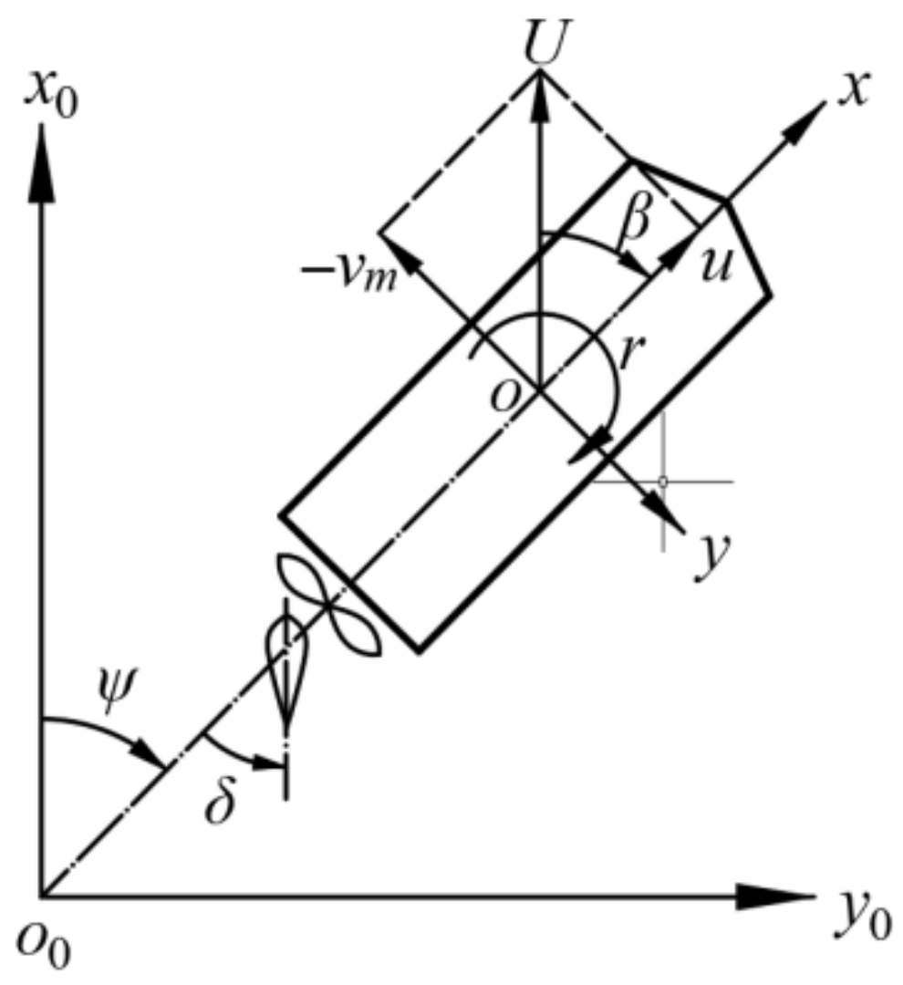
Considering 3-DOF ship maneuvering motion (surge, sway, and yaw) in the horizontal plane, two right-handed coordinate systems, a space-fixed coordinate system o0-x0y0z0 and a ship-fixed coordinate system o-xyz, were adopted, as shown in Figure 1. Both the plane o0-x0y0 and the plane o-xy were located at the undisturbed free surface. The z0-axis pointed downward. The origin of the ship-fixed coordinate system was located at the midship, and the x-axis was pointing to bow, the y-axis to starboard, and the z-axis downward. , , and represented the surge velocity, lateral velocity, and yaw rate, respectively. The translational velocity was defined as =. The heading angle was defined as the angle between x0-axis and x-axis, and the drift angle was defined as =. The rudder angle was defined as positive when the rudder turns to the starboard.

Figure 1.
Coordinate systems.
2.2. Motion Equations
The MMG standard model proposed by Yasukawa and Yoshimura [30] is given as
where is the ship mass, and are the added masses in surge motion and sway motion; is the moment of inertia around the vertical axis passing through the center of gravity of the ship, and is the corresponding added moment of inertia. is the longitudinal coordinate of the center of gravity. , , and are the hydrodynamic surge force, lateral force, and yaw moment, which are decomposed into three parts:
where the subscripts H, R, and P denote the hydrodynamic forces and moments on the bare hull, rudder, and propeller. The detailed expressions of these forces and moments are given in Yasukawa and Yoshimura [30].
2.3. Hydrodynamic Forces on Bare Hull
In this paper, the forces and moments were non-dimensionalized by and respectively, the mass and moment of inertia were non-dimensionalized by and respectively, where is the density of water, is the ship length between perpendiculars, and is the draft.
The hydrodynamic forces and moment acting on bare hull were expressed as follows (Yasukawa and Yoshimura [30]):
where and are the non-dimensional lateral velocity and yaw rate; , , and are the non-dimensional hydrodynamic forces and moment expressed as polynomial functions:
where is the ship resistance coefficient in straight ahead motion; , , , etc. are the non-dimensional hydrodynamic derivatives.
2.4. Hydrodynamic Forces on Rotating Propeller
The hydrodynamic force on a working propeller was described as follows (Yasukawa and Yoshimura [30]):
where is the thrust deduction factor, is the propeller thrust expressed as
where is the propeller revolution; is the propeller diameter; is the thrust coefficient in open-water, which can be further expressed as a polynomial function of the propeller advance coefficient :
where the coefficients , , and can be determined by Least Square Method (LSM) based on the propeller open-water characteristics, and the propeller advance coefficient is defined as
where is the wake fraction at propeller plane in maneuvering motion. In this paper, the formula in Yasukawa and Yoshimura [30] was adopted:
where is the wake fraction at propeller plane in straight ahead motion, is the geometrical inflow angle to propeller in maneuvering motion, and are constants representing the wake characteristics in maneuvering motion. The wake characteristics at propeller plane are asymmetric about for a single screw ship, and takes different magnitudes at positive and negative . is expressed as
where is the non-dimensional longitudinal coordinate of the propeller plane.
2.5. Hydrodynamic Forces on Rudder
The hydrodynamic forces acting on the rudder can be written as (Yasukawa and Yoshimura [30]):
where is the steering resistance deduction factor, is the rudder force increase factor, and are the longitudinal coordinates of the rudder position and the acting point of the additional lateral force due to rudder deflection, respectively. , , and are collectively referred to as hull-rudder interaction coefficients. is the rudder normal force expressed as
where is the profile area of the movable part of rudder, is the resultant inflow velocity to rudder, is the rudder lift gradient coefficient, is the effective inflow angle at the rudder. In this paper, Fujii’s formula (Fujii and Tuda [31]) was used to estimate . , , and are expressed as follows:
where is the rudder aspect ratio; and are the longitudinal and lateral velocity components of inflow to rudder, expressed as
where is the ratio of the wake fractions at propeller and rudder positions, is the ratio of propeller diameter to rudder height, is a constant; is the flow straightening coefficient, is the effective inflow angle to rudder in maneuvering motion. Because of the asymmetrical flows in port side and starboard, takes different magnitudes in positive and negative . is expressed as
where is the non-dimensional effective longitudinal coordinate of rudder position.
3. Geometry of the Target Ship
In this study, all the virtual captive model tests were carried out for a fully appended KVLCC2 ship model, one of the well-known benchmark hull forms. The geometry of the KVLCC2 ship model is shown in Figure 2. The principal particulars of the KVLCC2 model are listed in Table 1. There were two different scale ratios used in the present study for the purpose of comparison with the test data of different institutes from various aspects. The scale ratio used in the virtual captive model tests was 1:46.4, the same as that used in the physical captive model tests by the Hyundai Maritime Research Institute (HMRI). The propeller revolution = 9.9 rps and ship speed = 1.1702 m/s were also consistent with the model tests of HMRI. To compare with the data of free-running model tests (FRMTs) conducted by Maritime Research Institute Netherlands (MARIN), the scale ratio of 1:45.7, the same as that of the FRMTs, was used in the maneuvering predictions.

Figure 2.
Geometry of the fully appended KVLCC2 ship model.

Table 1.
Principal particulars of KVLCC2 ship models with different scale ratios.
4. Numerical Methods
In this study, computations were performed by using the Reynolds-averaged Navier–Stokes (RANS) solver in STAR-CCM+. The governing equations were closed with the Shear Stress Transport (SST) turbulence model. The Finite Volume Method (FVM) was used to discretize the flow domain. The temporal discretization was based on a first-order fully implicit scheme, and the spatial discretization was performed with the second-order upwind scheme for the convection term and the secondary gradient contribution for the diffusion term. The Semi-Implicit Method for Pressure-Linked Equations (SIMPLE) algorithm was employed for pressure-velocity coupling. Moreover, the free surface was captured with the Volume of Fluid (VOF) method. The Dynamic Fluid Body Interaction (DFBI) method was used to simulate the ship motion.
4.1. Computational Domain and Boundary Conditions
As depicted in Figure 3, a cuboid computational domain was adopted. The coordinate system was defined with the x-axis pointing to bow, y-axis to starboard, and z-axis downward. The origin was located at the intersection of the water-line plane and the center-line plane at the midship. The dimension of the computational domain ranges −4.0 < x < 2.5, −2.0 < y < 2.0, and −0.2 < z < 1.0. The computational domain was composed of two parts. One was the background domain which contained the entire computational domain except for a small cylindrical domain containing the propeller, while the other was a small cylindrical domain adopted to embed the propeller and to simulate the propeller rotation.
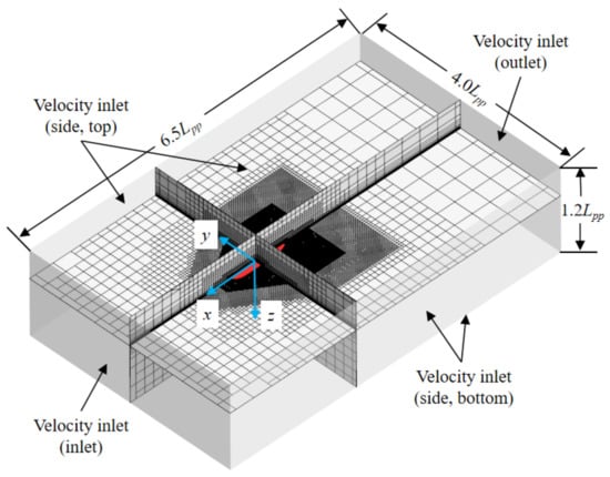
Figure 3.
Computational domain and boundary conditions.
As for the boundary conditions, the velocity inlet boundary condition was imposed on the boundaries of the background domain to describe the far-field condition. The wave damping with a length of 1.2 was set on the boundaries of the background domain except for the top and bottom boundaries to reduce the wave reflections from the boundaries. The interface boundary conditions were imposed on the contact surfaces between the cylindrical domain and the background domain. The no-slip wall boundary condition was imposed on the solid surfaces of hull, rudder, and propeller.
4.2. Mesh Generation
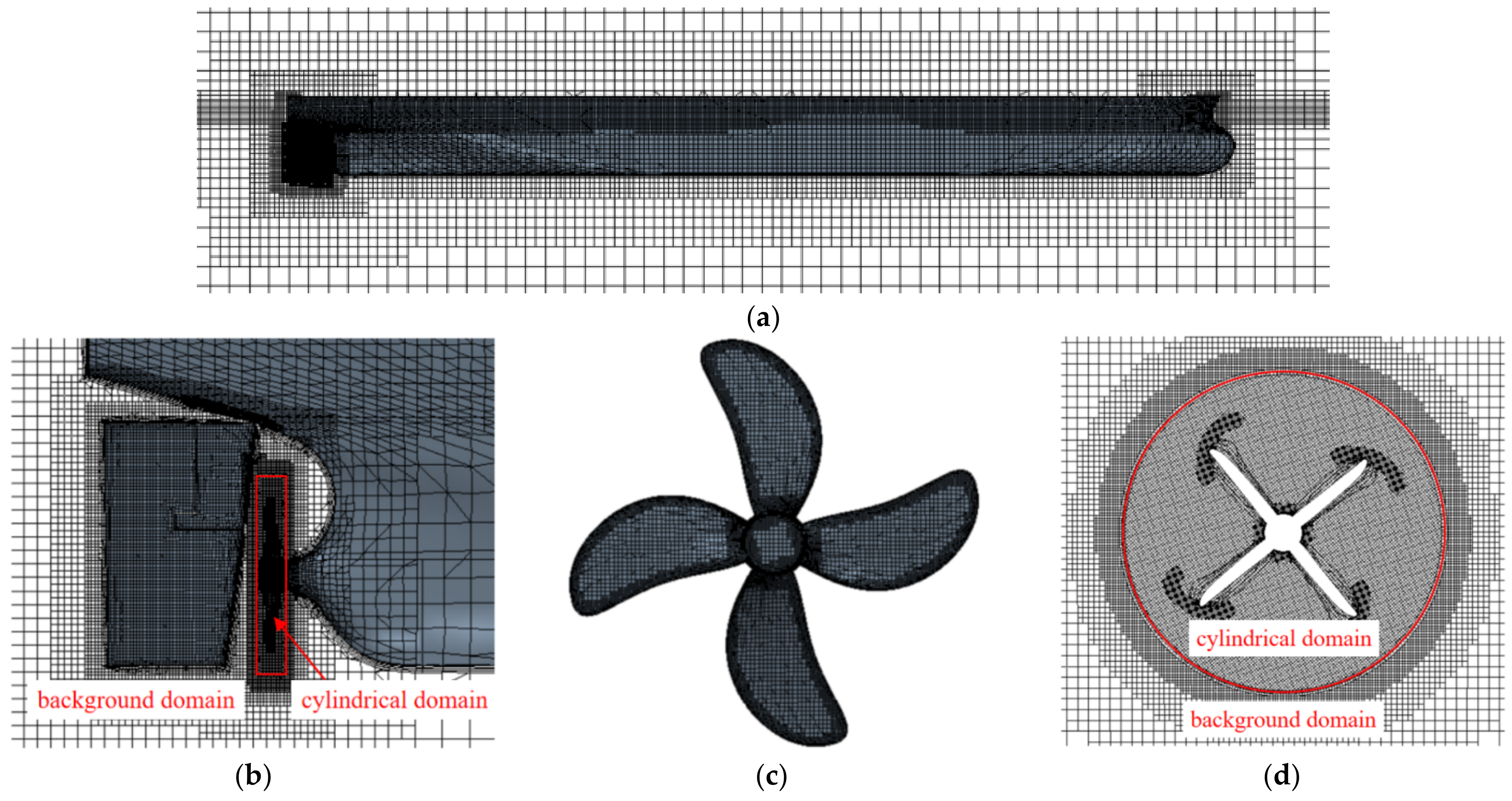
The computational domain was discretized by unstructured hexahedral meshes, and denser meshes around the free surface, bow, stern, rudder, and propeller were adopted to capture the flow and wave features during ship motion more precisely. To resolve the near-wall and boundary-layer flows, the all-y+ wall treatment was utilized, and y+ values were controlled around 23 throughout all simulations by setting an appropriate near-wall thickness. To eliminate the differences of the meshes in the MRF and SM methods, the meshes keep the same in all simulations. Figure 4 shows the details of mesh distribution.
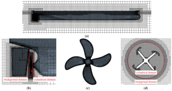
Figure 4.
Mesh distributions. (a) Side view of the mesh around the hull; (b) Meshes around the stern; (c) Surface meshes of the propeller; (d) Meshes at the propeller plane.
4.3. Propeller Modeling Methods
The same division of the computational domains was adopted for the MRF and the SM propeller modeling methods: a cylindrical domain containing the propeller and a background domain covering the global domain; thus, the same meshes can be used for both methods. An interface between the cylindrical domain and the background domain was required to transmit the information of flow variables across the interface.
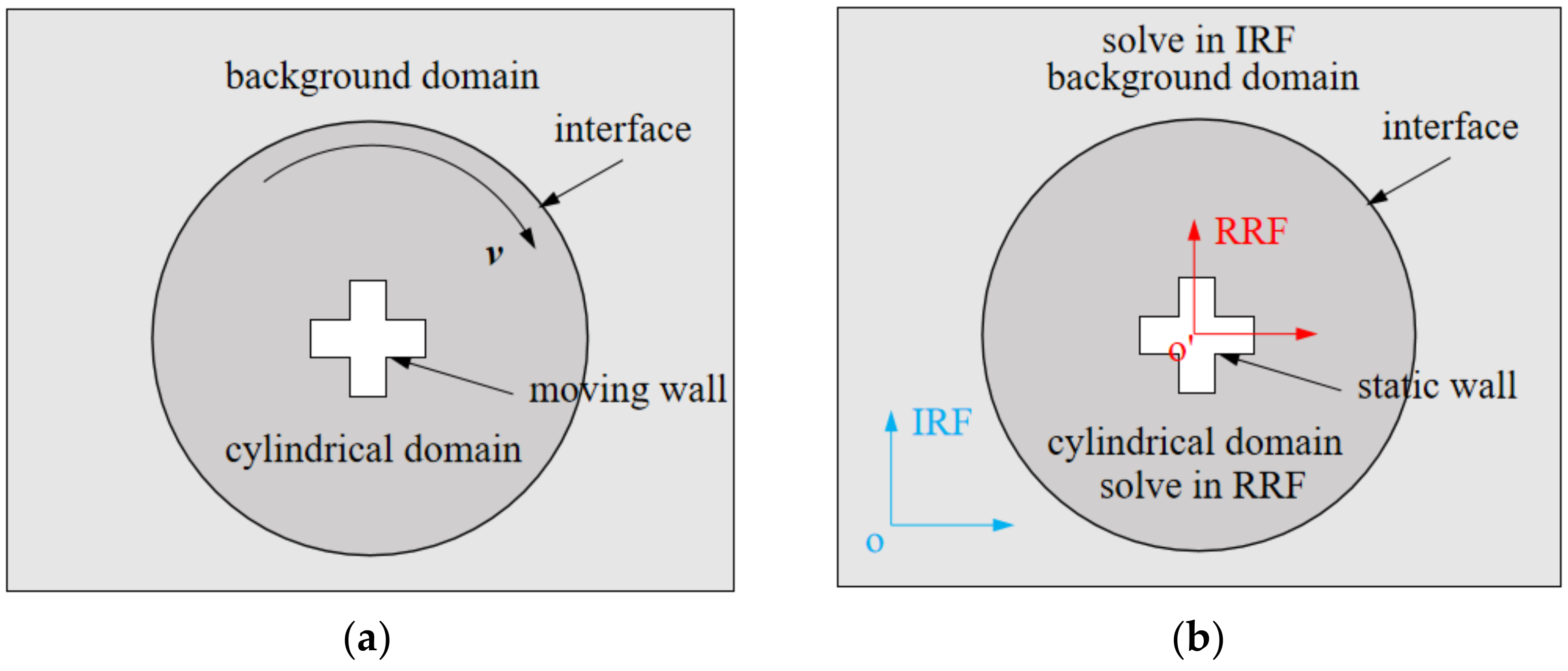
The MRF method and the SM method are different in the process of simulating the propeller rotation. The SM method is a transient method where both the propeller and its surrounding meshes in the cylindrical domain actually rotate with the propeller shaft (as shown in Figure 5a). However, the cylindrical domain remains stationary in the MRF method, where the flow field in the background domain is solved by the governing equations in the inertial reference frame (IRF), while the effects of rotating propeller are simulated by solving the governing equations in the rotating reference frame (RRF) in the cylindrical domain. The details of governing equations in IRF to RRF can be found in Pauli et al. [18]. Through the corresponding mathematical transformation between the two reference frames and the data interpolation between the cylindrical domain and the background domain, the numerical simulations of the flow field and the rotation motion are realized. The schematic diagram of the MRF method is shown in Figure 5b.
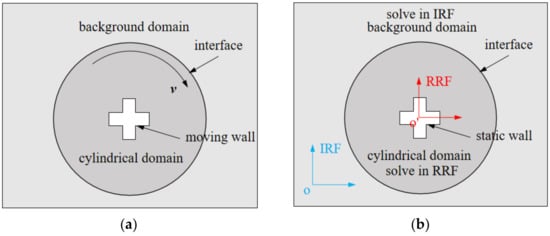
Figure 5.
Schematic diagram of SM and MRF methods. (a) SM method; (b) MRF method.
5. Numerical Error and Uncertainty Analysis
The Grid Convergence Index (GCI) method (Celik et al. [32]) based on Richardson extrapolation (Richardson [33]; Richardson and Gaunt [34]) was used to estimate the numerical error and uncertainty due to the discretization in CFD computations. A brief introduction to its application process is given below:
Firstly, three sets of discretization sizes (for mesh and time step) are selected for simulation. The sizes of the three sets are , , and < < , corresponding to the fine, medium, and coarse ones. The refinement factor is defined as = = = = ; , , and represent the solutions of , , and . The convergence ratio is defined as (Stern et al. [35]):
where = − denotes the change between medium-fine solutions; = − denotes the change between coarse-medium solutions.
The possible convergence states are:
- (1)
- Monotonic Convergence (MC): 0 < < 1.
- (2)
- Oscillatory Convergence (OC): < 0; < 1.
- (3)
- Monotonic Divergence (MD): > 1.
- (4)
- Oscillatory Divergence (OD): < 0; > 1.
Then, the apparent order of the method is expressed as (Celik et al. [32])
Next, the extrapolated value is calculated with
Finally, the following error estimates are calculated and reported, along with the apparent order :
For approximate relative error:
For extrapolated relative error:
For the fine-grid convergence index:
A convergence study of mesh and time step discretizations was carried out based on the above approach. Taking a rudder force test ( = 0°, = 0, = 25°) and an oblique towing test ( = 20°, = 0, = 0°) as examples, the impact of mesh and time-step discretizations on the prediction of ship hydrodynamic performance was analyzed. Three sets of mesh were generated to study the convergence of mesh discretization based on a uniform refinement factor of . The cell numbers in the cylindrical domain were 2.02 × 10⁵, 4.07 × 10⁵, and 8.57 × 10⁵ for the coarse, medium, and fine mesh sizes, respectively. The corresponding cell numbers in the background domain were 0.68 × 10⁶, 1.33 × 10⁶, and 2.72 × 10⁶. Three sets of time step were used to study the convergence of time step discretization based on a uniform refinement factor of 2. The time steps of MRF method were 5.05 × 10⁻² s, 2.53 × 10⁻² s, and 1.26 × 10⁻² s; the time steps of SM method were 5.61 × 10⁻⁴ s, 2.81 × 10⁻⁴ s, and 1.40 × 10⁻⁴ s. The convergence study of mesh discretization was conducted with the medium time step, while the convergence study of time step discretization was conducted with the medium mesh size. The discretization errors and uncertainties estimated from the convergence studies are given in Table 2, Table 3, Table 4 and Table 5, where “RFT” denotes the rudder force test, “OTT” denotes the oblique towing test.

Table 2.
The discretization error and uncertainty in spatial convergence study (MRF method).

Table 3.
The discretization error and uncertainty in temporal convergence study (MRF method).

Table 4.
The discretization error and uncertainty in spatial convergence study (SM method).

Table 5.
The discretization error and uncertainty in temporal convergence study (SM method).
Table 2 and Table 3 present the calculated discretization errors and uncertainties by MRF method. All the coefficients have small and in spatial convergence, while in oblique towing tests is more sensitive to the mesh resolutions as its is up to 25.18%. The in spatial convergence is less than 12%. All the coefficients have small and in temporal convergence, while in oblique towing tests is more sensitive to the time step as its is up to 51.75%. The in temporal convergence is less than 10%, except for in oblique towing tests (about 267%) with an oscillatory convergence.
Table 4 and Table 5 present the calculated discretization errors and uncertainties by SM method. All the coefficients have small and in spatial convergence, while in oblique towing tests is more sensitive to the mesh resolutions because its is up to 16.37%. The in spatial convergence is less than 6% except for in oblique towing tests (about 24%). All the coefficients have small and in temporal convergence, while in oblique towing tests is more sensitive to the time step because its is up to 29.39%. The in temporal convergence is less than 2% except for in oblique towing tests (about 112%).
The abnormal , , and in these tables are mainly due to the oscillatory convergence of numerical results, where the corresponding R values are beyond the range of (0, 1), implying that the GCI method is not applicable for such non-monotonic convergence cases. In general, the numerical convergence of the two propeller modeling methods is acceptable. Making a trade-off between the computational efficiency and computational accuracy, the medium mesh and the medium time step are used in the subsequent computations.
6. Results and Discussion
Before carrying out the maneuvering predictions, some necessary parameters needed to be determined. In Table 6, , , and were taken from Yasukawa and Yoshimura [30]; the value of was derived from Equation (14); and are the non-dimensional longitudinal coordinates of rudder and propeller; , , and were derived from the propeller open-water tests of HMRI [36].

Table 6.
Related parameters in the MMG model.
6.1. Resistance and Self-Propulsion Tests
Table 7 presents (1 − ) and (1 − ) obtained from the simulations of resistance and self-propulsion tests by using the MRF and SM methods, and the numerical results were compared with the available model test data and other CFD results in the literature. Parameters CFD-MRF and CFD-SM denote the present results obtained by the MRF and SM methods, respectively. Parameter EFD-HMRI represents the model test data of HMRI (SIMMAN2022 [36]; Shin et al. [37]; Sung and Park [38]); EFD-NMRI represents the model test data of National Maritime Research Institute (NMRI) (Yasukawa and Yoshimura [30]; SIMMAN2008 [39]); CFD-BF-NMRI denotes the CFD results of NMRI by using BF method (Sakamoto et al. [16]). It should be noted that the CFD solver, mesh distribution, and numerical discretization adopted in this paper and those in Sakamoto et al. [16] were not exactly the same. In addition, a horn rudder was considered in the present study, while a rudder without horn was used in Sakamoto et al. [16].

Table 7.
Parameters of resistance and self-propulsion tests obtained from experiments and simulations.
As shown in Table 7, the calculated (1 − ) and (1 − ) by the SM method presented higher accuracy comparing with the test data than those by the MRF and BF methods, as the relative error between the SM results and the test data is within 3%. The reason for the larger relative error of MRF method is that this method underestimates the propeller thrust, and the predicted ship propulsion point might be larger than the test data of HMRI. The underestimation of propeller thrust by the MRF method will be analyzed in the next subsection.
6.2. Rudder Force Tests
For the rudder force tests ( = 0°, = 0, ≠ 0°), Equation (2) can be rewritten in the non-dimensional form:
Equation (24) shows that (1 − ), (1 + ), and ( + ) are defined as the slopes of , , versus , , and , respectively.
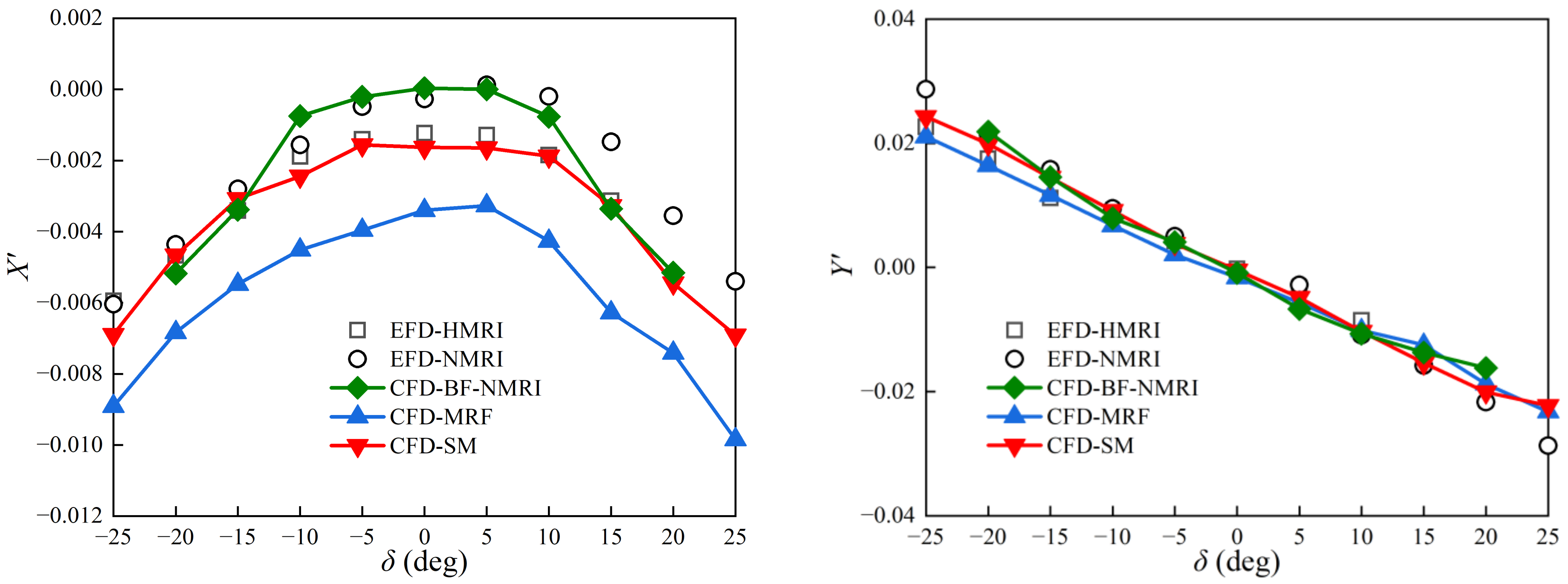
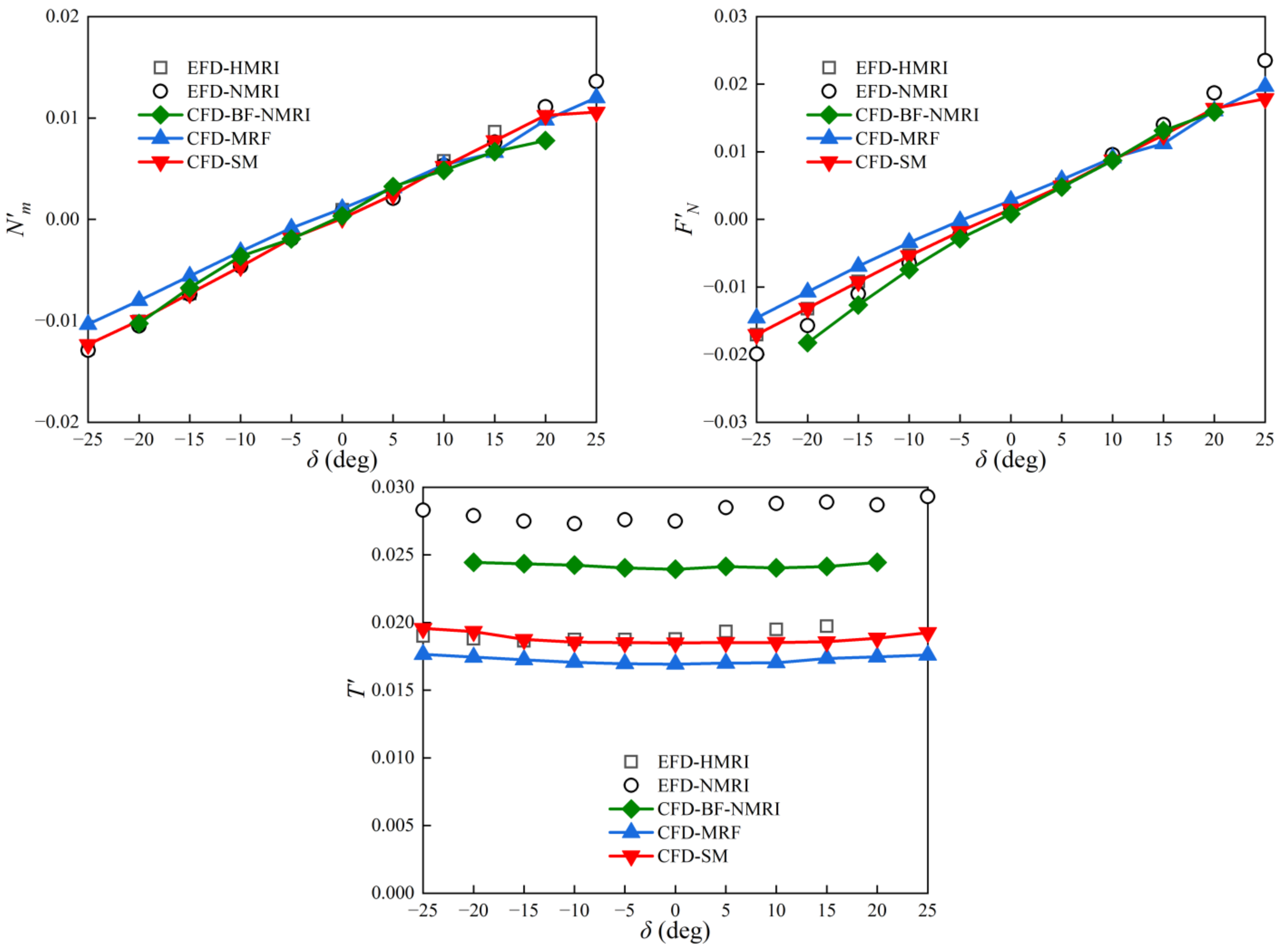
Figure 6 illustrates the CFD results of rudder force tests in comparison with the model test data. The value of calculated by the SM method was in better agreement with the test data than that by the MRF method. The result by the MRF method was generally larger than that by the SM method due to the fact that contains component, and the underestimated by the MRF method gives rise to a larger . There was a satisfactory consistency between the CFD results by the SM/MRF methods and the test data in terms of except for the case at = 25°. The accuracy of predicted and by the SM method was generally higher than those by the MRF and BF methods except for the case at = 25°. The more remarkable deviation at = 25° may be caused by the severe flow separation at a large rudder angle. The reason for a smaller obtained by the SM and MRF methods than that of NMRI is that the scale ratio and self-propulsion point in the present study are different from those of NMRI, and the similar observations are presented in the following paragraphs.
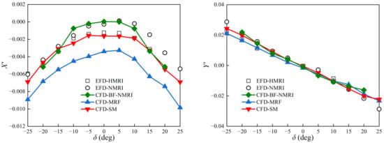
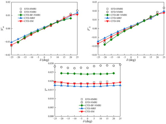
Figure 6.
Hydrodynamic quantities in rudder force tests obtained from experiments and simulations.
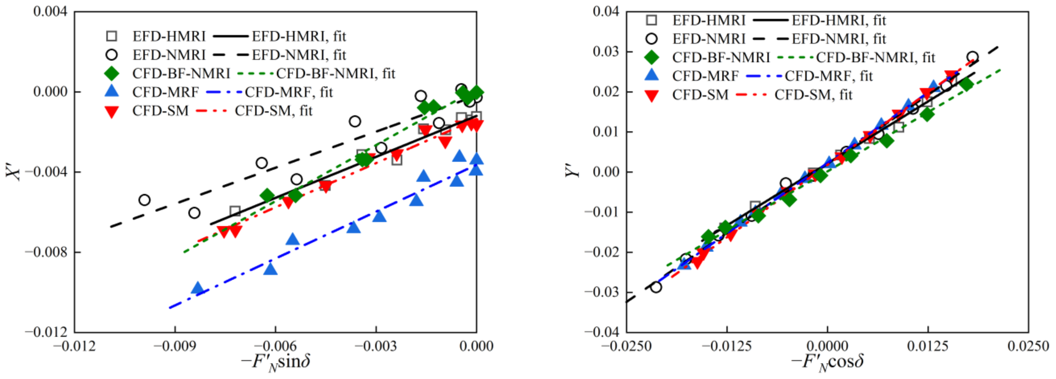
Figure 7 shows the plots of linear regression analysis to determine the hull-rudder interaction coefficients. These coefficients are summarized in Table 8. The calculated (1 − ) by the SM method presented the best consistency with the model test data among the three propeller modeling methods, and the result was about 19% larger than the test data. The calculated (1 + ) by the SM and MRF methods were 12% larger than the test data. The calculated ( + ) by the MRF and SM methods were in better agreement with the test data than that by the BF method. Although the accuracy of by the SM method was generally higher than that by the MRF method as shown in Figure 6, the hull-rudder interaction coefficients obtained by the two methods indicated that the difference in the interaction coefficients was minor.
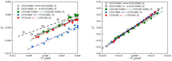
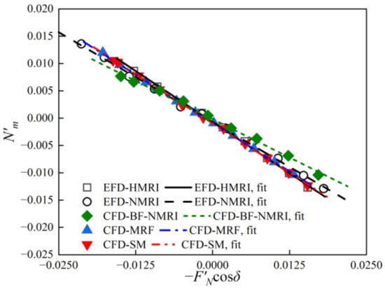
Figure 7.
Results of linear regression analysis for hull-rudder interaction coefficients.

Table 8.
The hull-rudder interaction coefficients obtained from the rudder force tests.
6.3. Oblique Towing Tests
The ship hydrodynamic forces measured in the oblique towing tests (OTTs) and circular motion tests (CMTs) by NMRI/HMRI contained inertia components, while in CFD simulations these forces were not considered. For the sake of direct comparisons between the CFD results and the test data, the inertia components (Yasukawa and Yoshimura [30]) were added to the computed hydrodynamic forces to obtain the surge force , lateral force , and yaw moment containing the inertia components:
where , , and are the hydrodynamic forces and moment on the hull including the inertia components:
Because the rudder angle is zero in OTTs and CMTs, Equation (25) can be rewritten as
Substituting Equation (26) into Equation (4) yields:
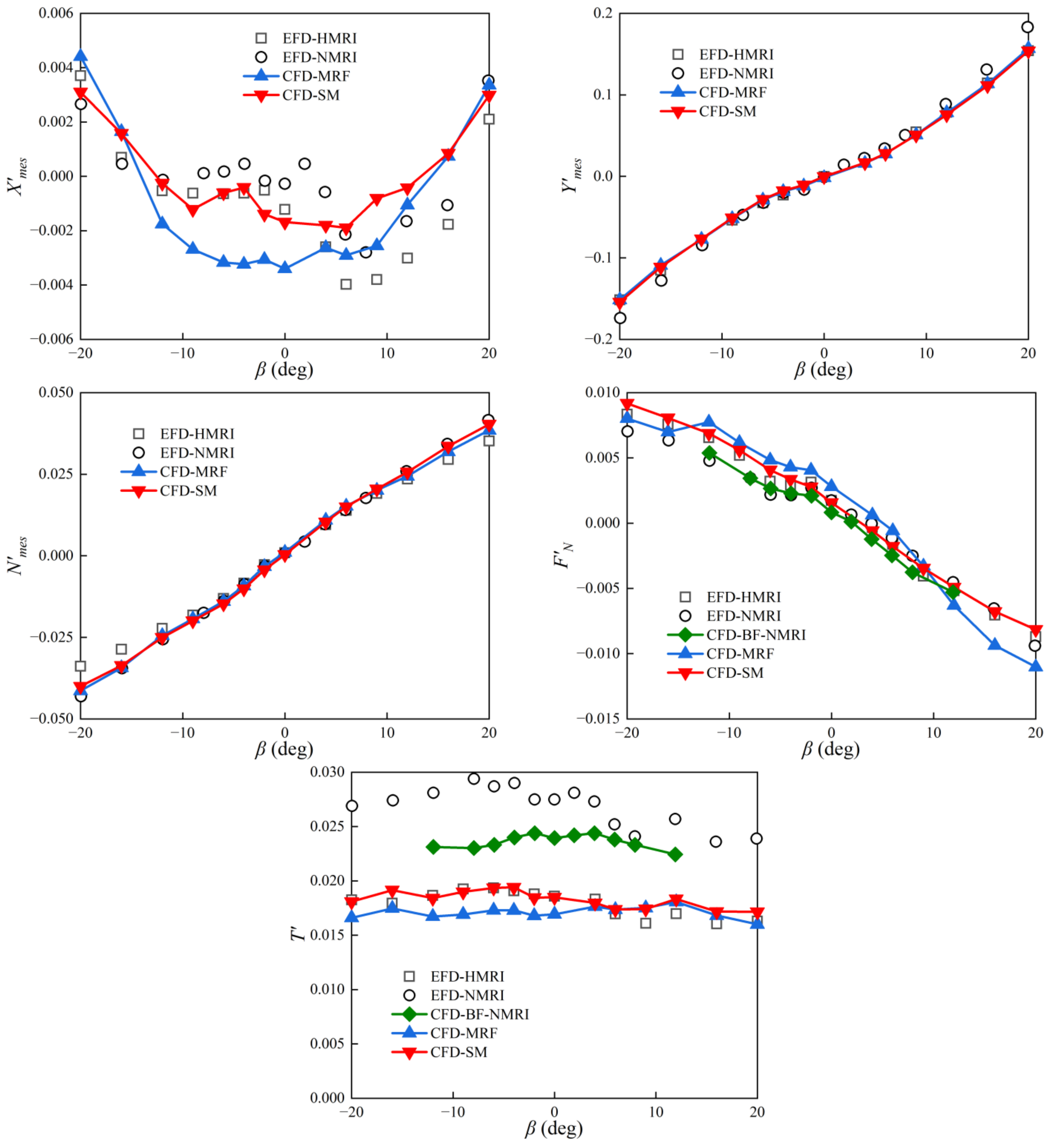
The simulation condition of OTTs is ≠ 0°, = 0, = 0°. Figure 8 shows the CFD results and the model test data of OTTs. The values of and calculated by the SM method were in good agreement with the test data of HMRI at < 0°, although some discrepancies were observed at > 0°. The SM method can capture the asymmetric characteristics of longitudinal forces (including and ) better than the MRF and BF methods, but still underestimated the asymmetric characteristics compared with the test data. A satisfactory agreement between the CFD results and the test data in terms of and was observed. The CFD results of were in better agreement with the test data of HMRI, while the results of were in better agreement with the test data of NMRI. The calculated by the SM method presented a good agreement with the test data, and some discrepancies were found in the calculated by the MRF method.
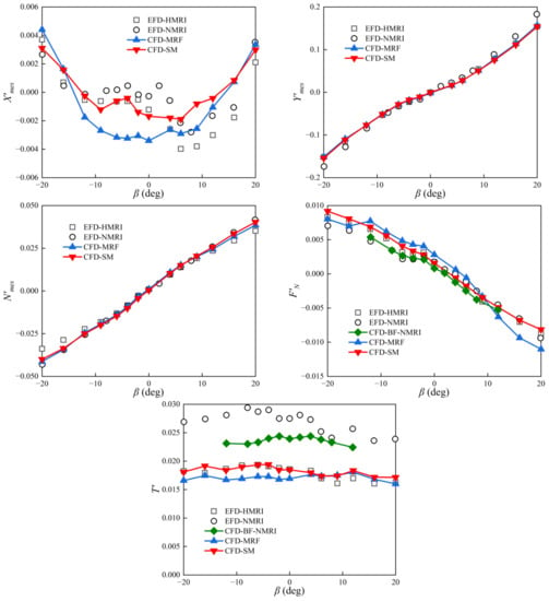
Figure 8.
Hydrodynamic quantities in OTTs obtained from experiments and simulations.
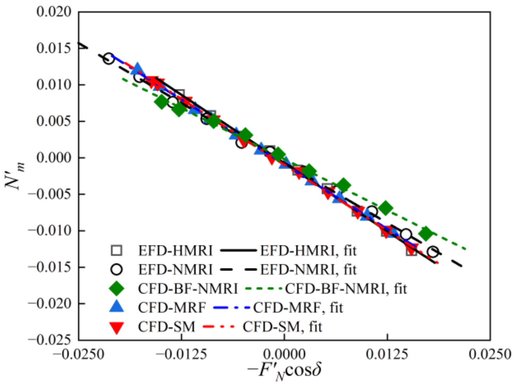
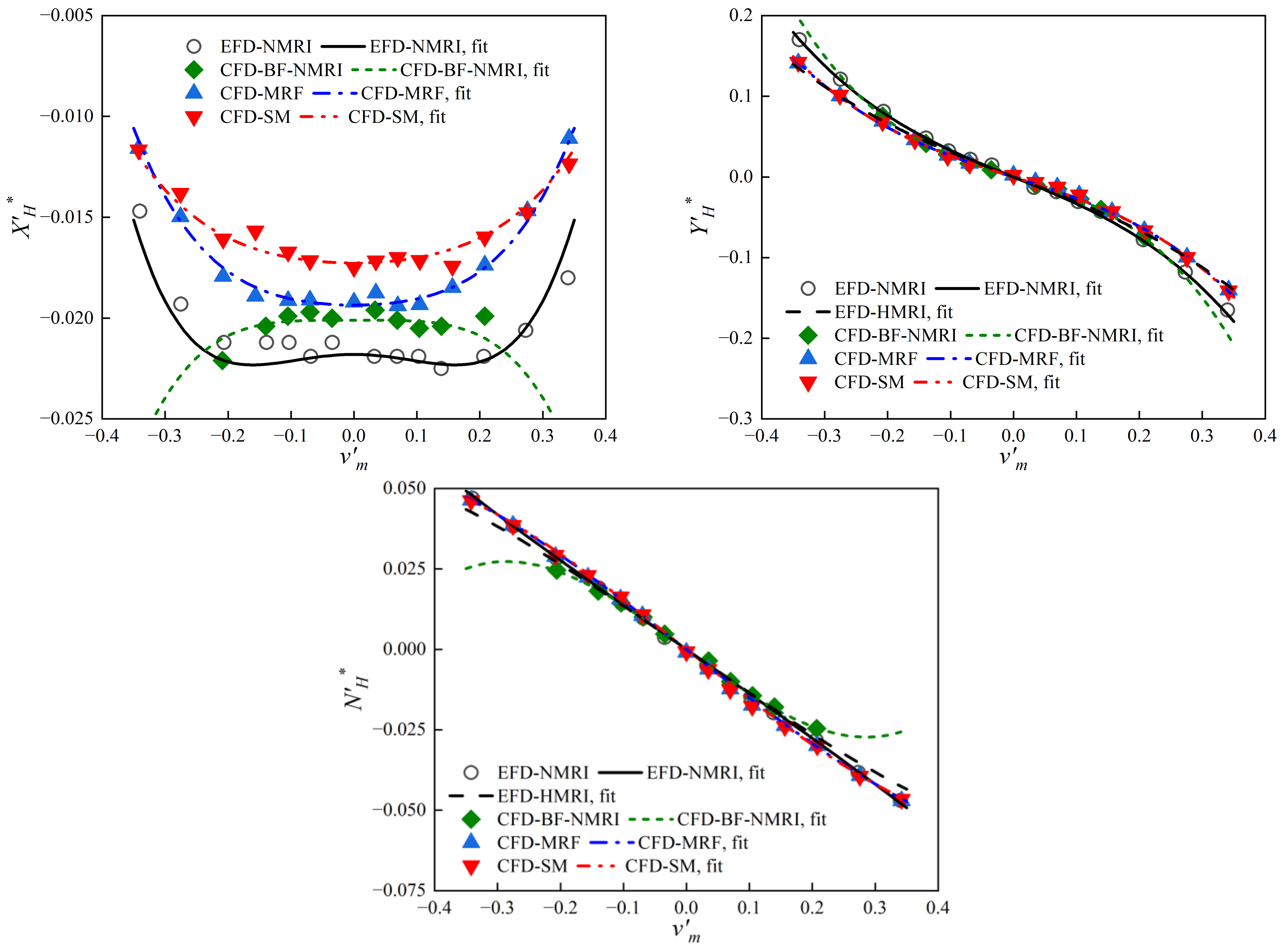
Figure 9 shows , , and obtained from OTTs and the corresponding fitting curves by LSM regression. Although and in Figure 8 are asymmetric with respect to , in Figure 9 is almost an even function of (or ). The value of calculated by the MRF method showed the best agreement with the test data among the three propeller modeling methods. The overall trend of calculated by the SM method was like the test data, but the trend of by the BF method was contrary to the test data. The calculated and by the SM and MRF methods showed good agreement with the test data. The fitting curve of the calculated by the BF method deviated from the test data at large drift angles, because the OTTs with large drift angles were not considered in Sakamoto et al. [16].
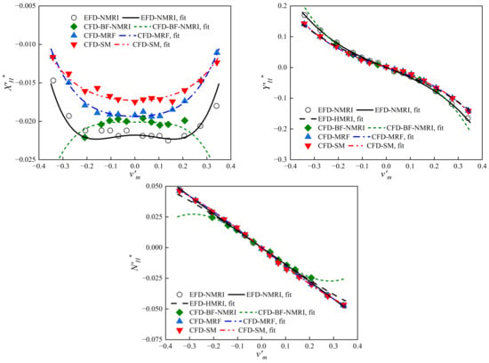
Figure 9.
Hydrodynamic forces on the hull obtained from OTTs and corresponding fitting curves.
The hydrodynamic derivatives obtained from the OTTs are listed in Table 9. There was little difference between the calculated hydrodynamic derivatives obtained by the SM method and the MRF method, and their results were all in good agreement with the test data except for the hydrodynamic derivatives related to the longitudinal motion and . The deviation of the longitudinal hydrodynamic derivatives was caused by the underestimated as shown in Figure 9. The values of calculated by the SM and MRF methods were about 17% larger than the test data of HMRI, and calculated by the two methods were about 75% smaller than the test data of HMRI, yet the fitting curves of the calculated by the two methods (Figure 9) were still in good agreement with the test data of HMRI.

Table 9.
Resistance coefficient and hydrodynamic derivatives obtained from OTTs.
6.4. Circular Motion Tests (β = 0°)
The simulation condition of circular motion tests (CMTs) ( = 0°) is ≠ 0, = 0°. Figure 10 shows the CFD results and the test data of CMTs. The overall trends of and calculated by the SM and MRF methods were consistent with those of the test data, and the values of and were smaller than the test data. The calculated and were in good agreement with the test data. The value of obtained by the SM method was in good agreement with the test data, while some significant deviation occurs in the calculated by the MRF method. All the three propeller modeling methods can capture the asymmetric characteristic of with respect to .
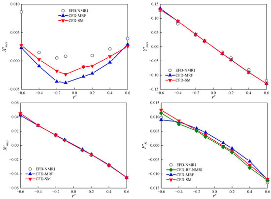
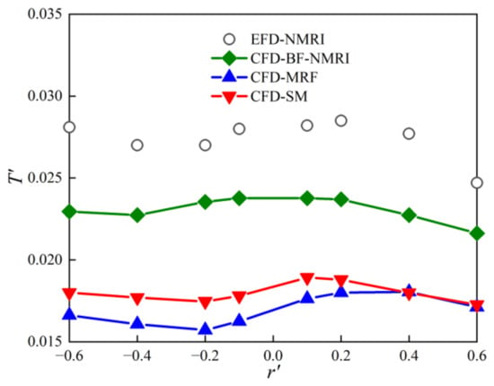
Figure 10.
Hydrodynamic quantities in CMTs (β = 0°) obtained from experiments and simulations.
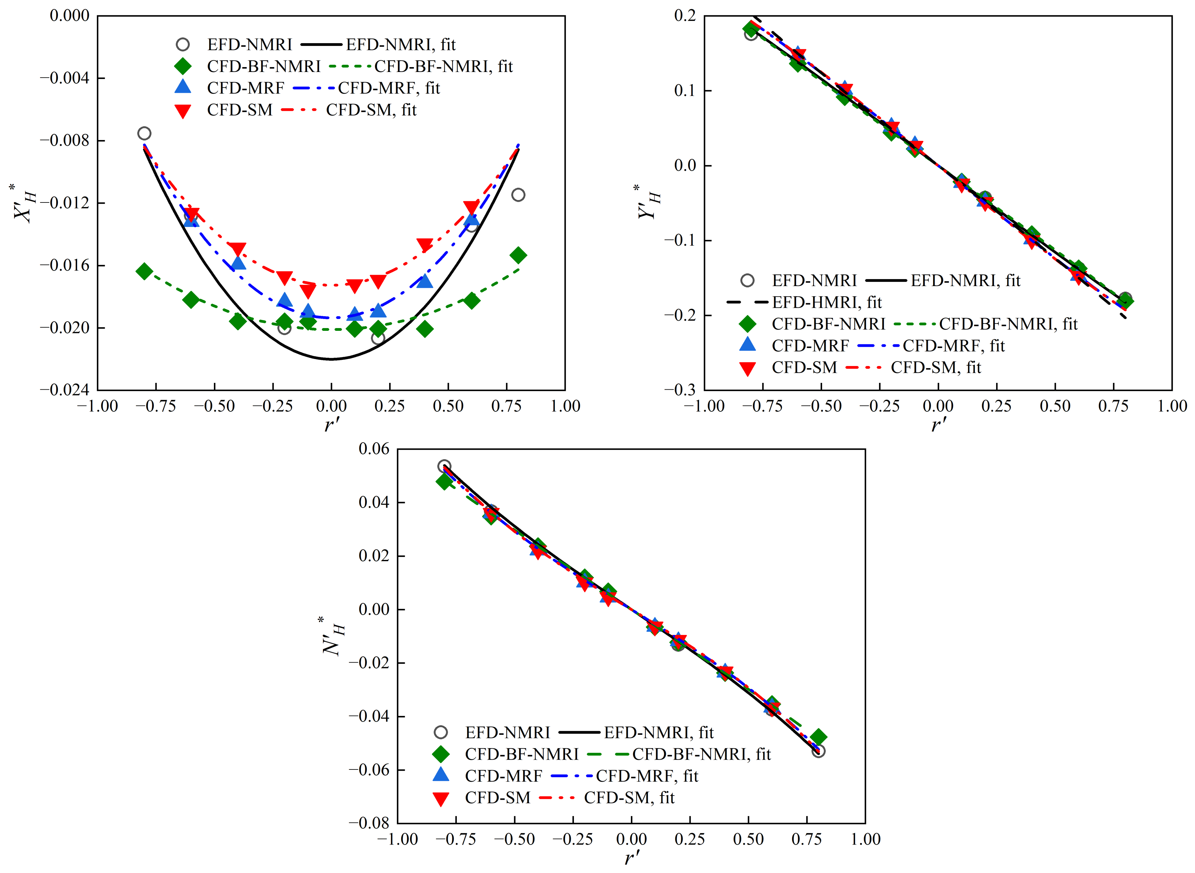
Figure 11 shows , , and obtained from CMTs ( = 0°) and the corresponding fitting curves by LSM regression. The hydrodynamic derivatives obtained from CMTs are listed in Table 10. Figure 11 shows that the calculated by the SM and MRF methods showed better agreement with the test data than that by the BF method, and were generally smaller than the test data. The calculated and by the three propeller modeling methods all agreed well with the test data. Table 10 shows that the hydrodynamic derivatives obtained by the SM and MRF methods agreed well with the test data.
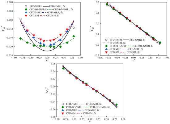
Figure 11.
Hydrodynamic forces on the hull obtained from CMTs (β = 0°) and corresponding fitting curves.

Table 10.
Hydrodynamic derivatives obtained from CMTs (β = 0°).
6.5. Circular Motion Tests (β ≠ 0°)
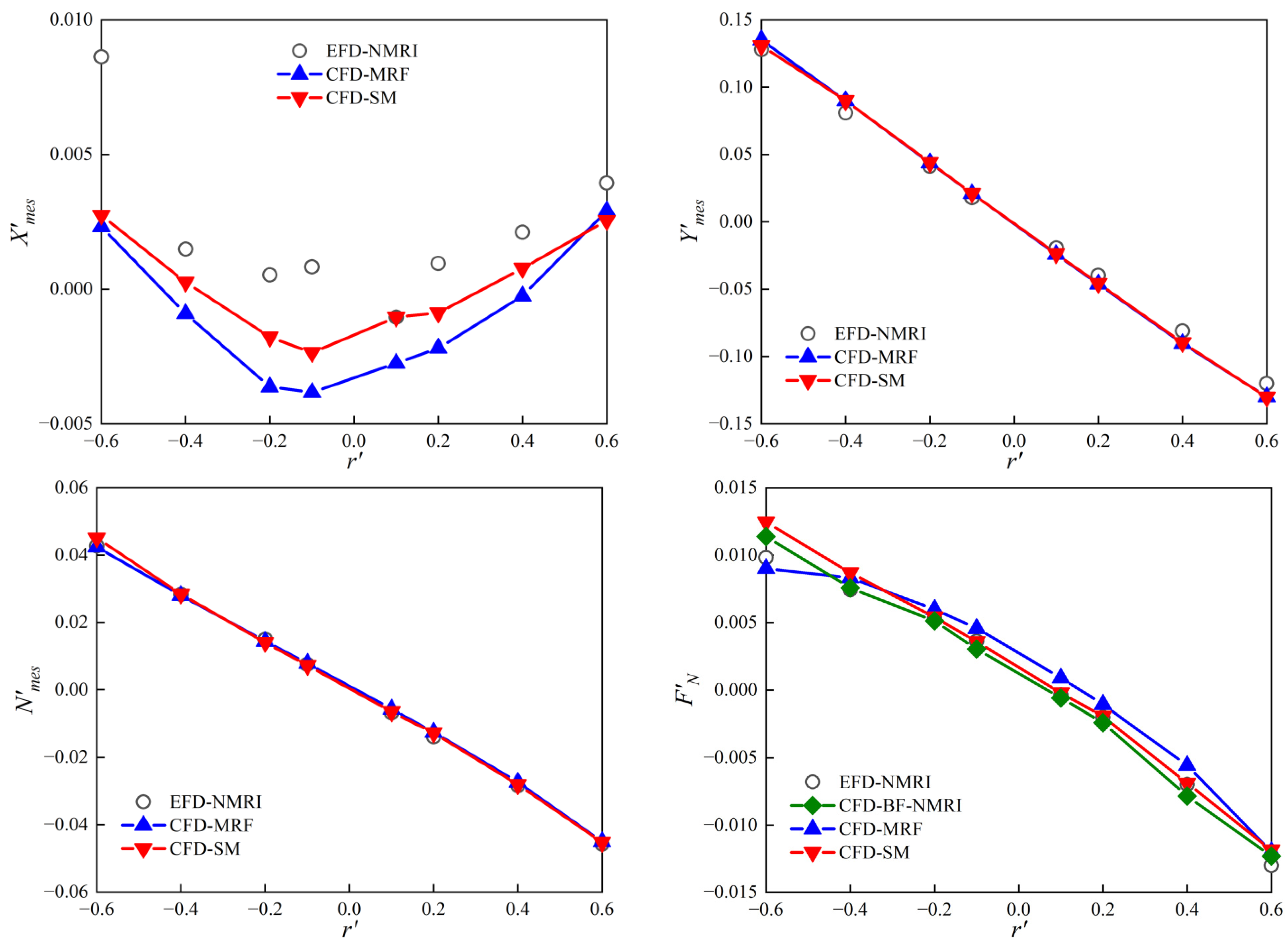
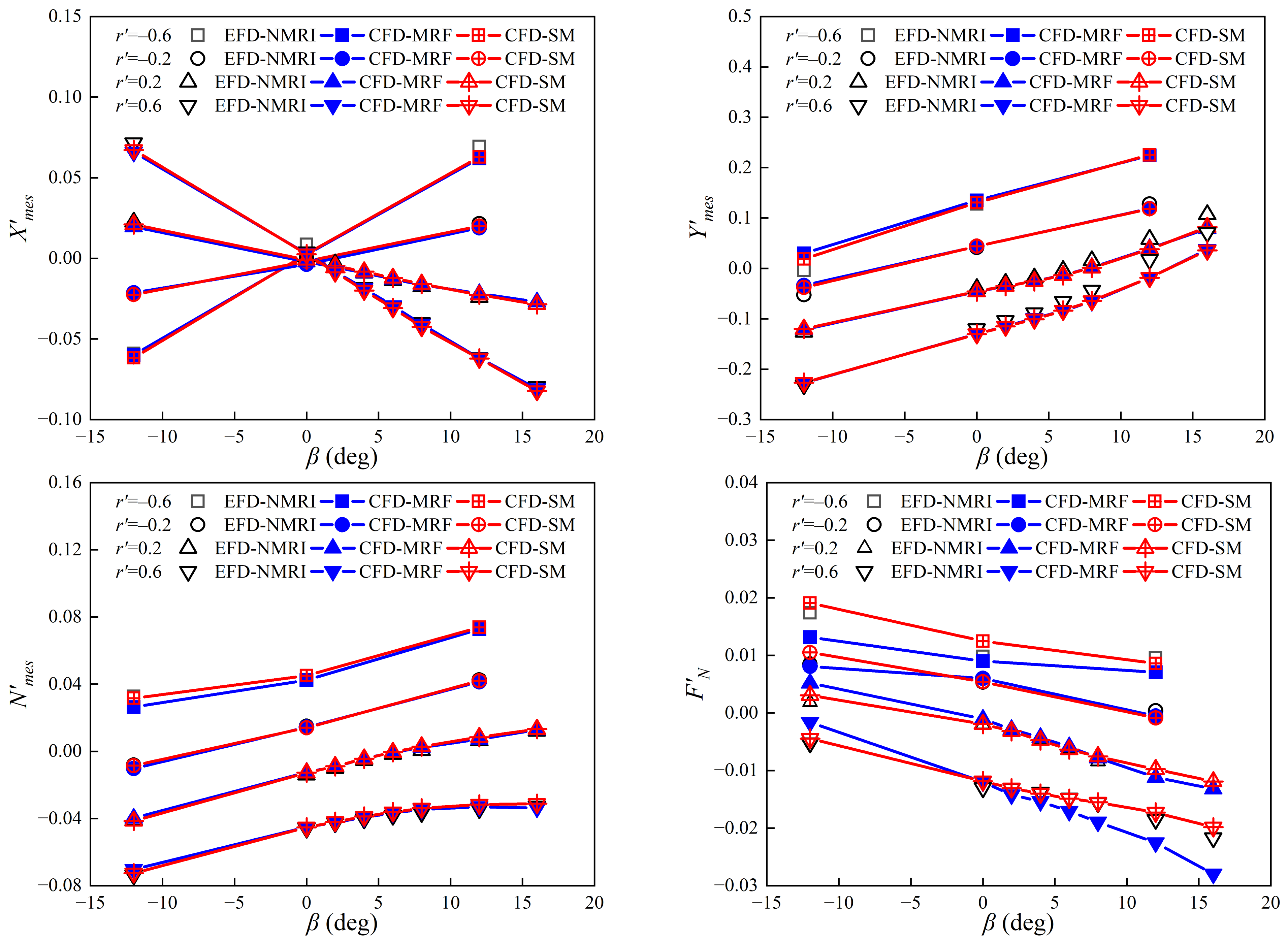
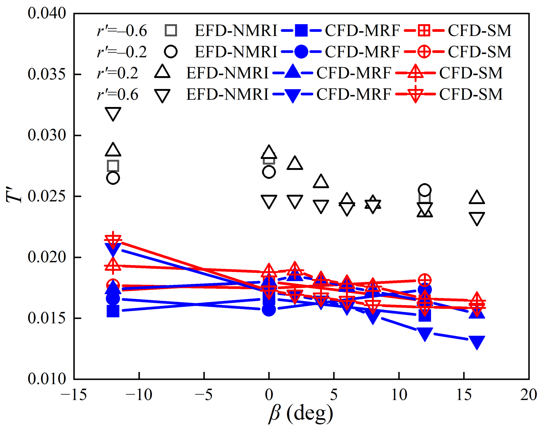
Figure 12 shows the CFD results of CMTs ( ≠ 0°) compared with the model test data. The calculated and were in good agreement with the test data. Generally, presents a satisfactory agreement with the test data, although there were larger discrepancies at the drift angles > 5° and larger yaw rate ( = 0.6). The value of calculated by the SM method was in better agreement with the test data than that by the MRF method, especially when the magnitude of yaw rate was larger ( = ±0.6).
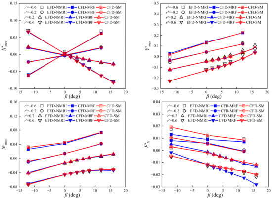
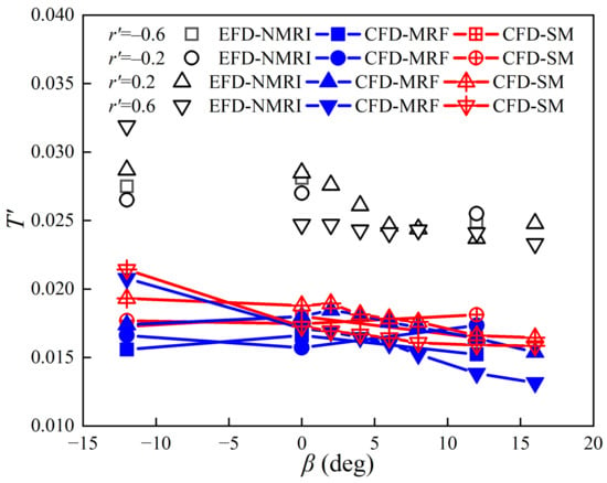
Figure 12.
Hydrodynamic quantities in CMTs (β ≠ 0°) obtained from experiments and simulations.
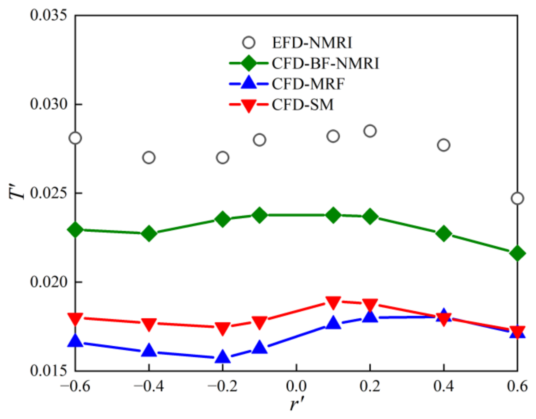
Figure 13 shows , , and obtained from CMTs ( ≠ 0°) and the corresponding fitting curves by LSM regression. The wake fraction was determined by the thrust identity method. Figure 14 shows and the corresponding fitting curves. The calculated presented obvious asymmetric tendencies versus , agreeing well with the test data at < 0°. The calculated by the SM method showed better agreement with the test data than that by the MRF method. Even so, remarkable deviations from the test data still existed at > 0° due to the complicated flow field and severe flow separations around the propeller under maneuvering condition.
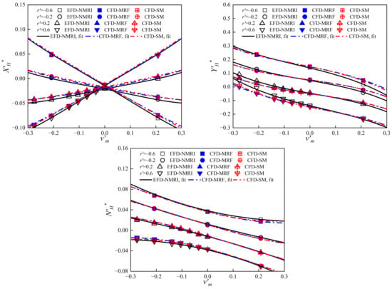
Figure 13.
Hydrodynamic forces on the hull obtained from CMTs (β ≠ 0°) and corresponding fitting curves.
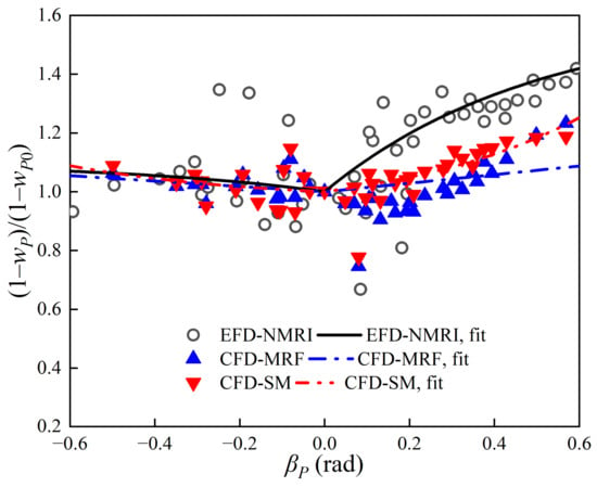
Figure 14.
Wake fraction and corresponding fitting curves.
Table 11 presents the hydrodynamic derivatives obtained from CMTs ( ≠ 0°), together with and . The calculated and by the SM method were more consistent with the test data than those by the MRF and BF methods. The calculated and by the SM and MRF methods were more consistent with the test data than those by the BF method. The deviation of and resulted from the underestimated at > 0°, as shown in Figure 14.

Table 11.
Cross hydrodynamic derivatives obtained from CMTs (β ≠ 0°), C1, and C2.
6.6. Oblique Towing and Steady Turning Tests with Rudder Angle
The simulation conditions of oblique towing and steady turning tests with rudder angle were ( ≠ 0°, = 0, ≠ 0°) and ( = 0°, ≠ 0, ≠ 0°), respectively. In addition to Equation (16), and can also be expressed as (Yasukawa and Yoshimura [30]):
where is the rudder angle at which the rudder normal force becomes zero.
Assume that is consistent with the test data of NMRI. By substituting obtained from Equation (29) into Equation (16), in Equation (16) can be determined by LSM regression.
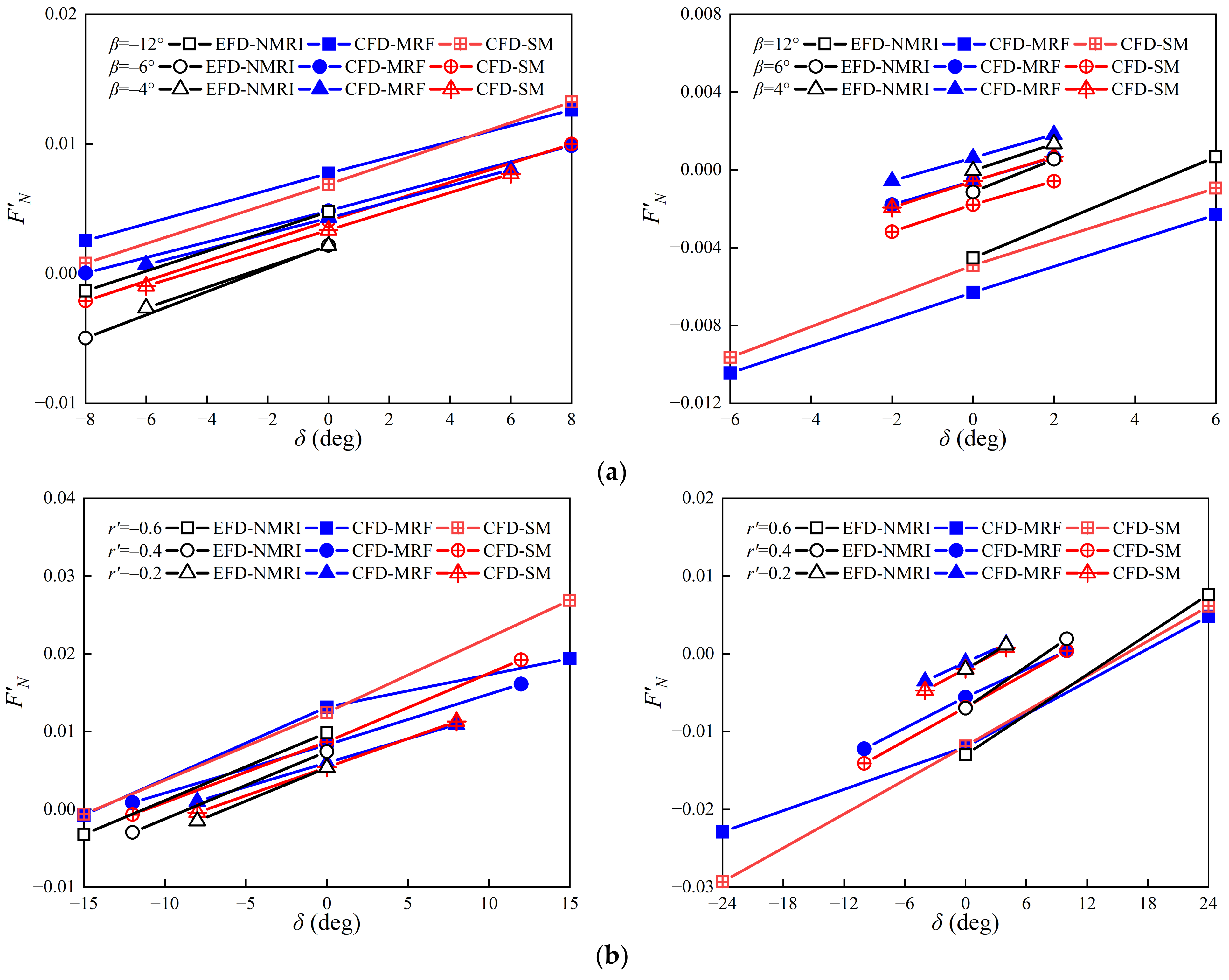
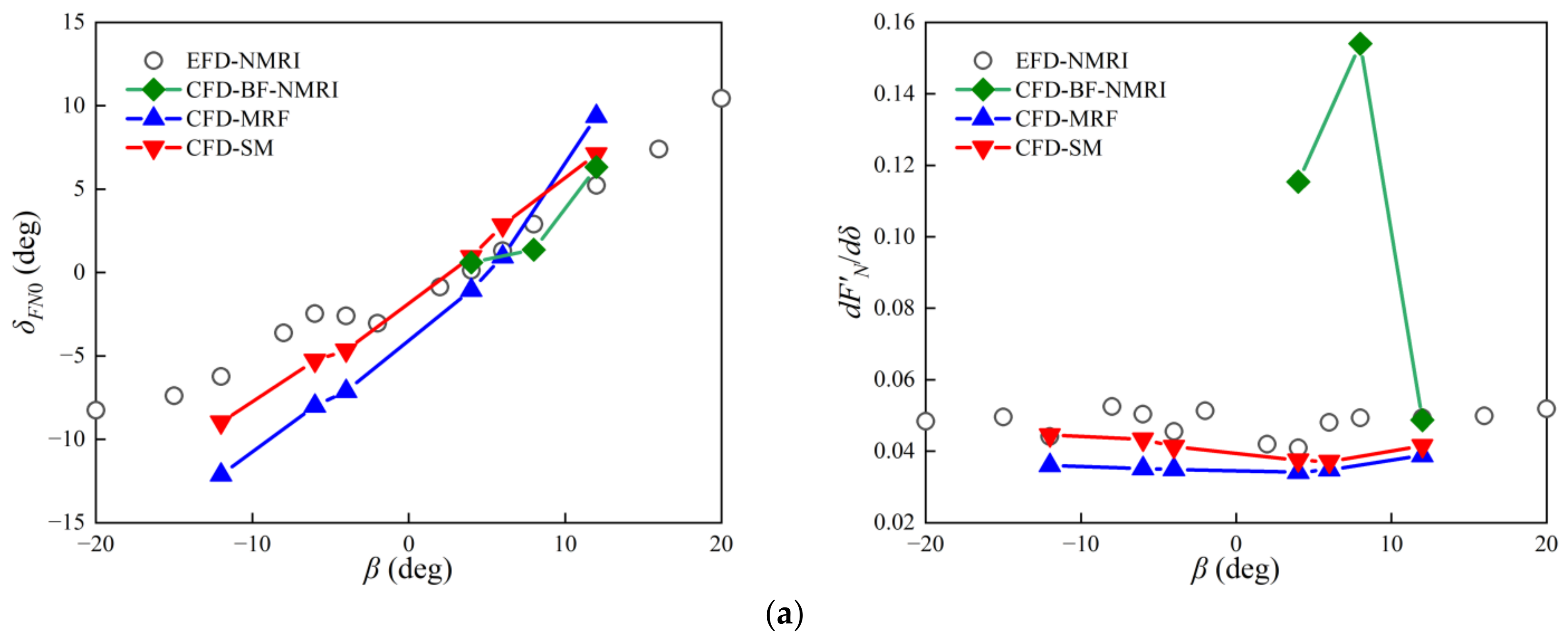
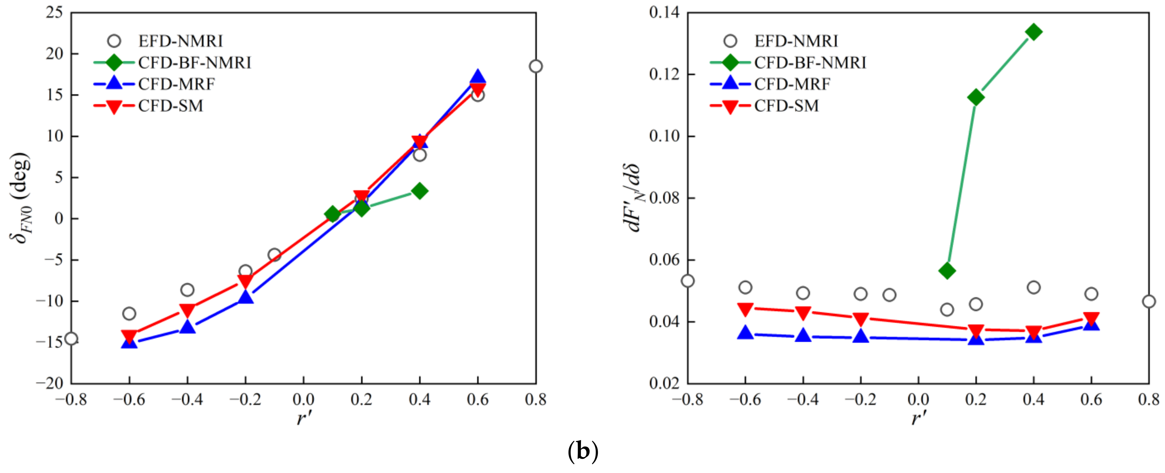
Figure 15 shows the CFD results of from oblique towing and steady turning tests with rudder angle in comparison with the test data. The calculated by the SM method was more consistent with the test data than that by the MRF method. Figure 16 shows and obtained by processing rudder normal forces in Figure 15. The calculated by the SM method was in better agreement with the test data than those by the MRF and BF methods. The calculated by the SM and MRF methods was slightly smaller than the test data, and the results obtained by the SM method agreed better with the test data, whereas was more overestimated by the BF method.
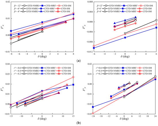
Figure 15.
Rudder normal force obtained from oblique towing and steady turning tests with rudder angle. (a) Rudder normal forces in oblique towing test with rudder angle; (b) Rudder normal forces in steady turning test with rudder angle.
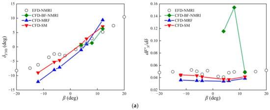
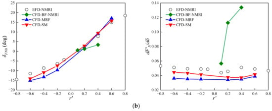
Figure 16.
δFN0 and dF’N/dδ obtained from oblique towing and steady turning tests with rudder angle. (a) Rudder parameters in oblique towing test with rudder angle; (b) Rudder parameters in steady turning test with rudder angle.
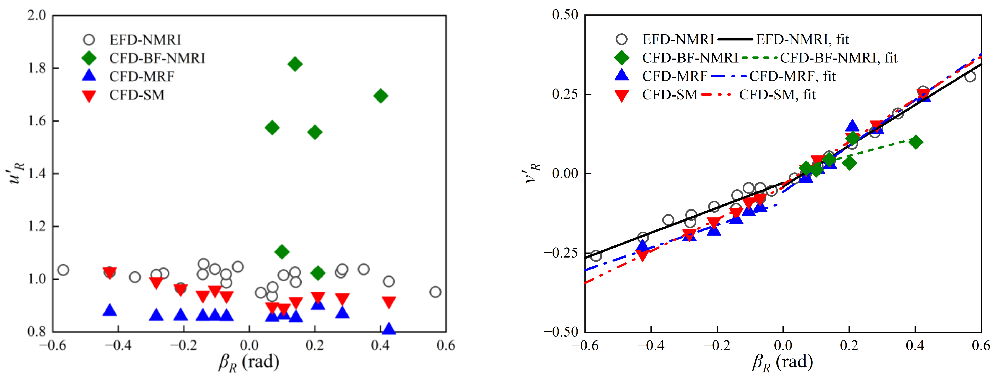
Figure 17 shows the calculated , and the linear regression of . It can be seen that obtained by the BF method was much larger than the test data, while the results obtained by the SM and MRF methods were slightly smaller than the test data. The values of obtained by the SM and MRF methods show obvious asymmetric characteristic against . A satisfactory consistency between the calculated by the SM/MRF methods and the test data at > 0° was observed, while significant deviation from the test data occurred at > 0° in the results obtained by the BF method. The calculated by the SM and MRF methods were slightly smaller than the test data at < 0°.
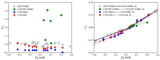
Figure 17.
Non-dimensional longitudinal and lateral inflow velocity components to rudder.
Table 12 presents the CFD results and the test data of and . The calculated by the MRF method showed higher accuracy comparing with the test data at < 0°, while the result by the SM method was in better agreement with the test data at > 0°. The discrepancy of the calculated by the BF method from the test data was more remarkable.

Table 12.
Rudder parameters determined by rudder force tests in oblique towing and steady turning motions.
In the present study, and in Equation (16) were estimated following the procedure in Yasukawa and Yoshimura [30]. However, and do not converge to the generally accepted values, which was also found in the study by Sakamoto et al. [16]. The values = 1.09 and = 0.50 in Yasukawa and Yoshimura [30] were used in the subsequent maneuvering simulations.
6.7. Maneuvering Simulations
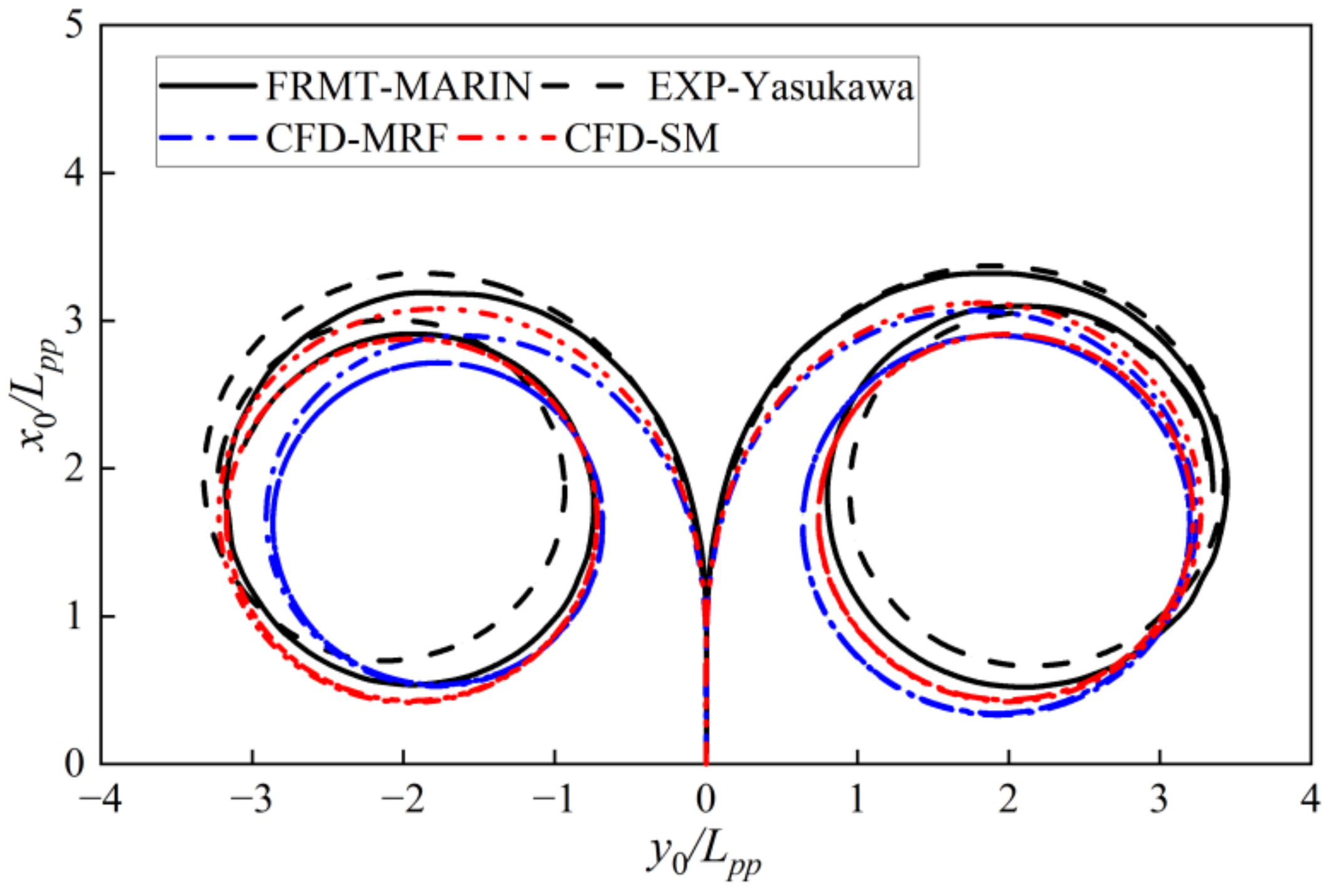
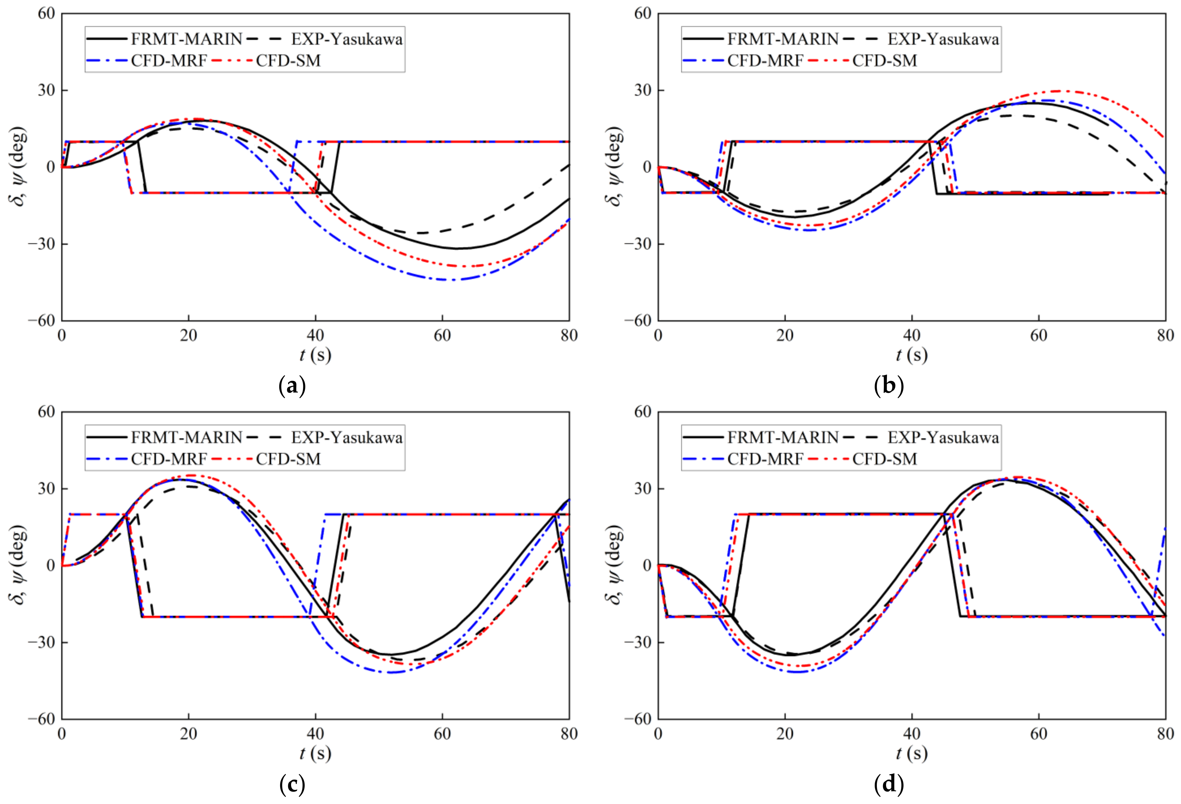
In order to compare the present results of maneuvering simulations with the free-running model test (FRMT) data of MARIN (denoted as FRMT-MARIN) (SIMMAN2008 [39]) and the system-based results utilizing the hydrodynamic derivatives and hull-propeller-rudder interaction coefficients obtained from the physical captive model tests (denoted as EXP-Yasukawa) (Yasukawa and Yoshimura [30]), the scale ratio 1:45.7 was selected for maneuvering simulations. The initial forward speed of the ship was = 1.179 m/s, and the rudder steering rate was 15.8 °/s. The propeller revolution was adjusted to allow the ship to move at the initial speed . Maneuvering motions were simulated by solving Equation (1) with a fourth-order Runge-Kutta scheme. The predicted trajectories of turning circle maneuvers under = ±35° are presented in Figure 18, and the results of ±10°/10° and ±20°/20° zig-zag maneuvers are presented in Figure 19. Table 13 summarizes the maneuvering parameters, i.e., the non-dimensional advance , the non-dimensional tactical diameter , and the first and second overshoot angles (OSAs), together with the relative error , defined as (Pred.–FRMT)%FRMT, where “Pred.” denotes the maneuvering parameters predicted by system-based methods.
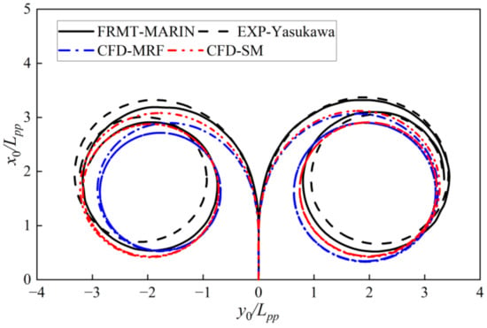
Figure 18.
Trajectories of ±35° turning circle maneuvers.
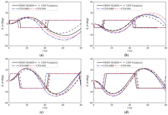
Figure 19.
Time histories of heading angle and rudder angle of zig-zag maneuvers. (a) +10°/10°; (b) −10°/10°; (c) +20°/20°; (d) −20°/20°.

Table 13.
Summary of maneuvering parameters.
As Figure 18 and Table 13 show, the accuracy of the predicted turning circle maneuvers by the SM method was higher than that by the MRF method. For the +35° turning circle maneuver, the results of the SM method showed slightly higher accuracy than those of the MRF method. The results of both the SM and MRF methods were in good agreement with the FRMT data, with the maximum relative error of 8.31%. For the −35° turning circle maneuver, the accuracy of the SM method (maximum relative error 3.86%) was clearly higher than that of the MRF method (maximum relative error 9.97%), and even slightly higher than the results of EXP-Yasukawa (maximum relative error 5.84%). Moreover, the turning ability of the KVLCC2 ship model was generally overestimated by the CFD methods, while mostly underestimated by EXP-Yasukawa.
As shown in Figure 19 and Table 13, the accuracy of the predicted zig-zag maneuvers by the SM method (average relative error 21.89%) was generally higher than that by the MRF method (average relative error 27.64%) except for the −10°/10° zig-zag maneuver, but slightly lower than that of EXP-Yasukawa (average relative error 20.13%). The yaw checking ability of the KVLCC2 ship model evaluated by the overshoot angles was generally underestimated by the CFD methods, while mostly overestimated by EXP-Yasukawa.
7. Conclusions
The RANS-based CFD method was applied to simulate the captive model tests of a fully appended KVLCC2 ship model by using the SM method and the MRF method for the propeller modelling. The hydrodynamic forces on the hull-propeller-rudder system, the hydrodynamic derivatives and hull-propeller-rudder interaction coefficients in the MMG model were computed, and the numerical results were validated against the available test data and the CFD results of BF method in the literature. The standard turning circle and zig-zag maneuvers were predicted by using the MMG model with the computed hydrodynamic derivatives and hull-propeller-rudder interaction coefficients, and the predicted maneuvering parameters were validated by comparing them with the FRMT data. Some conclusions can be drawn from this study:
- (1)
- In general, the results of ship hydrodynamic forces and maneuvering predictions obtained by the SM method were more accurate than those by the MRF and BF methods compared with the test data.
- (2)
- The lateral forces and yaw moments calculated by the SM, MRF, and BF methods were in good agreement with the test data. The rudder normal force calculated by the SM method was more accurate than those by the MRF and BF methods compared with the test data. The propeller thrust calculated by the SM method was more accurate than that by the MRF method compared with the test data, while the MRF method underestimated the propeller thrust.
- (3)
- It is more appropriate to adopt the MRF or the BF methods in simulations of OTTs and CMTs to save computing time with sufficient prediction accuracy of and , while it may be necessary to adopt the SM method in simulations of rudder force tests to obtain with higher accuracy.
- (4)
- The calculated wake fraction by the MRF and SM methods deviated from the test data at > 0°. To obtain with higher accuracy, more accurate turbulence flow simulation for the propeller is needed.
- (5)
- In general, the prediction accuracy of the standard maneuvers by the SM method was higher than that by the MRF method, but slightly lower than that of EXP-Yasukawa.
- (6)
- The turning ability of the KVLCC2 ship model was generally overestimated by the CFD methods but underestimated by EXP-Yasukawa. The yaw checking ability was underestimated by the CFD methods but overestimated by EXP-Yasukawa.
In future work, the prediction accuracy of the wake fraction can be improved by higher order turbulence modeling such as Detached Eddy Simulation or Large Eddy Simulation. The present work focused on 3-DOF maneuvering motion and neglected the roll effect; a 4-DOF MMG model will be adopted in a future study to consider the roll effect. Moreover, the added mass and added moment of inertia were estimated in the present work by using empirical formulae from the literature. The virtual Planar Motion Mechanism (PMM) test can be an option to determine the added mass and added moment of inertia accurately.
Author Contributions
Conceptualization, C.C. and Z.Z.; software, C.C. and H.G.; validation, C.C.; investigation, C.C.; resources, L.Z. and Z.Z.; writing—original draft preparation, C.C.; writing—review and editing, L.Z., Z.Z. and H.G.; supervision, L.Z. and Z.Z.; project administration, L.Z. and Z.Z.; funding acquisition, L.Z. and Z.Z. All authors have read and agreed to the published version of the manuscript.
Funding
This work is financially supported by the National Natural Science Foundation of China (Grant No. 51979164).
Institutional Review Board Statement
Not applicable.
Informed Consent Statement
Not applicable.
Data Availability Statement
Not applicable.
Acknowledgments
The authors thank SIMMAN Workshops for providing the model test data of KVLCC2.
Conflicts of Interest
The authors declare no conflict of interest.
Abbreviations and Nomenclature
| Abbreviations | |
| BF | Body Force |
| CFD | Computational Fluid Dynamics |
| CMT | Circular Motion Test |
| DFBI | Dynamic Fluid Body Interaction |
| FRMT | Free-running Model Test |
| FVM | Finite Volume Method |
| GCI | Grid Convergence Index |
| HMRI | Hyundai Maritime Research Institute |
| IRF | Inertial Reference Frame |
| ITTC | International Towing Tank Conference |
| LSM | Least Square Method |
| MARIN | Maritime Research Institute Netherlands |
| MMG | Maneuvering Modeling Group |
| MRF | Multiple Reference Frames |
| NMRI | National Maritime Research Institute |
| OSA | Overshoot Angle |
| OTT | Oblique Towing Test |
| PMM | Planar Motion Mechanism |
| RANS | Reynolds-averaged Navier-Stokes |
| RFT | Rudder Force Test |
| RRF | Rotating Reference Frame |
| SIMMAN | Workshop on Verification and Validation of Ship Maneuvering Simulation Methods |
| SIMPLE | Semi-Implicit Method for Pressure-Linked Equations |
| SM | Sliding Mesh |
| SST | Shear Stress Transport |
| VOF | Volume of Fluid |
| Nomenclature | |
| Non-dimensional advance | |
| Rudder force increase factor | |
| Profile area of movable part of rudder | |
| Ship breadth | |
| , | Constants representing the wake characteristics in maneuvering motion |
| Ship draft | |
| Propeller diameter | |
| Non-dimensional tactical diameter | |
| Relative error | |
| Approximate relative error | |
| Extrapolated relative error | |
| Rudder lift gradient coefficient | |
| Rudder normal force | |
| Fine-grid convergence index | |
| , , | Discretization sizes of fine, medium and coarse meshes/time steps |
| Rudder height | |
| Moment of inertia about the vertical axis passing through the left of gravity of the ship | |
| Propeller advance coefficient | |
| Added moment of inertia | |
| , , | Coefficients representing |
| Thrust coefficient in open-water | |
| Ship length between perpendiculars | |
| Non-dimensional effective longitudinal coordinate of rudder position | |
| Ship mass | |
| , | Added masses in surge and sway motions |
| Propeller revolution | |
| Apparent order | |
| Convergence ratio | |
| , , | Refinement factors |
| Ship resistance coefficient in straight ahead motion | |
| Propeller thrust | |
| Thrust deduction factor | |
| Steering resistance deduction factor | |
| Translational velocity | |
| , , | Surge velocity, lateral velocity and yaw rate |
| Resultant inflow velocity to rudder | |
| , | Longitudinal and lateral velocity components of inflow to rudder |
| Wake fraction at propeller plane in maneuvering motion | |
| Wake fraction at propeller plane in straight ahead motion | |
| , , | Surge force, lateral force and yaw moment |
| Longitudinal coordinate of the left of gravity | |
| Longitudinal coordinates of the acting point of the additional lateral force | |
| , , | Surge force, lateral force and yaw moment on bare hull |
| , , | Surge force, lateral force and yaw moment on the bare hull with the inertia components |
| , , | Surge force, lateral force and yaw moment with the inertia components |
| Surge force on propeller | |
| Non-dimensional longitudinal coordinate of the propeller plane | |
| Longitudinal coordinates of the rudder position | |
| , , | Surge force, lateral force and yaw moment on rudder |
| Effective inflow angle at the rudder position | |
| Drift angle | |
| Geometrical inflow angle to propeller in maneuvering motion | |
| Effective inflow angle to rudder in maneuvering motion | |
| Flow straightening coefficient | |
| Rudder angle | |
| Rudder angle at which the rudder normal force becomes zero | |
| Ratio of wake fractions at propeller and rudder positions | |
| , | Change between medium-fine solutions and change between coarse-medium solutions |
| Ratio of propeller diameter to rudder height | |
| A constant for expressing | |
| Rudder aspect ratio | |
| Scale ratio | |
| Density of water | |
| , , | Solutions of fine, medium and coarse meshes/time steps |
| Extrapolated value | |
| Heading angle | |
| Displacement volume | |
References
- ITTC Maneuvering Committee. Final Report and Recommendations to the 29th ITTC. In Proceedings of the 29th International Towing Tank Conference, Online, 13–18 June 2021.
- SIMMAN 2014. Available online: http://simman2014.dk/ (accessed on 19 June 2022).
- Abkowitz, M.A. Lectures on Ship Hydrodynamics—Steering and Manoeuvrability; Technical Report Rep. No. Hy-5; Hydro og Aerodynamisk Laboratorium: Lyngby, Denmark, 1964. [Google Scholar]
- Ogawa, A.; Koyama, T.; Kijima, K. MMG Report-I, On the mathematical model of ship manoeuvring. Bull. Soc. Nav. Archit. Jpn. 1977, 575, 22–28. (In Japanese) [Google Scholar]
- Cura-Hochbaum, A. On the numerical prediction of the ship’s manoeuvring behaviour. Ship Sci. Technol. 2011, 5, 27–39. [Google Scholar] [CrossRef]
- Shenoi, R.R.; Krishnankutty, P.; Selvam, R.P. Study of manoeuvrability of container ship by static and dynamic simulations using a RANSE-based solver. Ships Offshore Struct. 2016, 11, 316–334. [Google Scholar] [CrossRef]
- Liu, Y.; Zou, L.; Zou, Z.J.; Guo, H.P. Predictions of ship maneuverability based on virtual captive model tests. Eng. Appl. Comput. Fluid Mech. 2018, 12, 334–353. [Google Scholar] [CrossRef]
- Ardeshiri, S.; Mousavizadegan, S.H.; Kheradmand, S. Virtual simulation of PMM tests independent of test parameters. Brodogradnja 2020, 71, 55–73. [Google Scholar] [CrossRef]
- Seo, J.; Kim, D.H.; Ha, J.; Rhee, S.H.; Yoon, H.K.; Park, J.; Seok, W.; Rhee, K.P. Captive model tests for assessing maneuverability of a damaged surface combatant with initial heel angle. J. Ship Res. 2020, 64, 392–406. [Google Scholar] [CrossRef]
- Kim, H.; Akimoto, H.; Islam, H. Estimation of the hydrodynamic derivatives by RaNS simulation of planar motion mechanism test. Ocean. Eng. 2015, 108, 129–139. [Google Scholar] [CrossRef]
- Dai, K.; Li, Y.B. Manoeuvring prediction of KVLCC2 with hydrodynamic derivatives generated by a virtual captive model test. Pol. Marit. Res. 2019, 26, 16–26. [Google Scholar] [CrossRef]
- Dai, K.; Li, Y.B. Experimental and numerical investigation on maneuvering performance of small waterplane area twin hull. Brodogradnja 2021, 72, 93–114. [Google Scholar] [CrossRef]
- Franceschi, A.; Piaggio, B.; Tonelli, R.; Villa, D.; Viviani, M. Assessment of the manoeuvrability characteristics of a twin shaft naval vessel using an open-Source CFD code. J. Mar. Sci. Eng. 2021, 9, 665. [Google Scholar] [CrossRef]
- Kołodziej, R.; Hoffmann, P. Numerical estimation of hull hydrodynamic derivatives in ship maneuvering prediction. Pol. Marit. Res. 2021, 28, 46–53. [Google Scholar] [CrossRef]
- Mai, T.L.; Jeon, M.; Lim, S.H.; Yoon, H.K. Investigation of maneuvering characteristics of high-speed catamaran using CFD simulation. In Modern Mechanics and Applications; Springer: Singapore, 2022; pp. 546–559. [Google Scholar]
- Sakamoto, N.; Ohashi, N.; Araki, M.; Kume, K.; Kobayashi, H. Identification of KVLCC2 manoeuvring parameters for a modular-type mathematical model by RaNS method with an overset approach. Ocean. Eng. 2019, 188, 106257. [Google Scholar] [CrossRef]
- Farkas, A.; Degiuli, N.; Martić, I.; Dejhalla, R. Impact of hard fouling on the ship performance of different ship forms. J. Mar. Sci. Eng. 2020, 8, 748. [Google Scholar] [CrossRef]
- Pauli, L.; Both, J.W.; Behr, M. Stabilized finite element method for flows with multiple reference frames. Int. J. Numer. Methods Fluids 2015, 78, 657–669. [Google Scholar] [CrossRef]
- Song, S.; Demirel, Y.K.; Atlar, M. An investigation into the effect of biofouling on full-scale propeller performance using CFD. In Proceedings of the 38th International Conference on Ocean, Offshore and Arctic Engineering, Glasgow, Scotland, UK, 9–14 June 2019. [Google Scholar]
- Jin, Y.; Yiew, L.J.; Zheng, Y.; Magee, A.R.; Duffy, J.; Chai, S. Dynamic manoeuvres of KCS with CFD free-running computation and system-based modelling. Ocean. Eng. 2021, 241, 110043. [Google Scholar]
- Zhai, S.C.; Liu, D.C.; Han, Y.B. Numerical study of pressure fluctuation induced propeller cavitation with pre-shrouded vanes. J. Ship Mech. 2021, 25, 1292–1301. [Google Scholar]
- Wang, X.; Cai, F.; Shi, A.G.; Ying, R.R. Numerical simulation of the viscous flow over the ship with twin-propellers and twin-rudders in rotating arm tests. J. Ship Mech. 2014, 18, 786–793. (In Chinese) [Google Scholar]
- Guo, J.; Meng, K.; Chen, Z.; Dai, Y. Numerical calculation and analysis of self-propulsion power characteristics of waterjet driven ship. Shipbuild. China 2021, 62, 149–161. (In Chinese) [Google Scholar]
- Wang, C.; Sun, S.; Sun, S.; Li, L. Numerical analysis of propeller exciting force in oblique flow. J. Mar. Sci. Technol. 2019, 22, 602–619. [Google Scholar] [CrossRef]
- Guo, H.P.; Zou, Z.J. A RANS-based study of the impact of rudder on the propeller characteristics for a twin-screw ship during maneuvers. Ocean. Eng. 2021, 239, 109848. [Google Scholar] [CrossRef]
- Guo, H.P.; Zou, Z.J. CFD and system-based investigation on the turning maneuver of a twin-screw ship considering hull-engine-propeller interaction. Ocean. Eng. 2022, 251, 110893. [Google Scholar] [CrossRef]
- Jin, Y.; Duffy, J.; Chai, S.; Magee, A.R. DTMB 5415M dynamic manoeuvres with URANS computation using body-force and discretised propeller models. Ocean. Eng. 2019, 182, 305–317. [Google Scholar] [CrossRef]
- Yu, J.; Feng, D.; Liu, L.; Yao, C.; Wang, X. Assessments of propulsion models for free-running surface ship turning circle simulations. Ocean. Eng. 2022, 250, 110967. [Google Scholar] [CrossRef]
- Deng, G.B.; Queutey, P.; Wackers, J.; Visonneau, M.; Guilmineau, E.; Leroyer, A. Assessment of ship maneuvering simulation with different propeller models. J. Hydrodyn. 2022, 34, 422–433. [Google Scholar] [CrossRef]
- Yasukawa, H.; Yoshimura, Y. Introduction of MMG standard method for ship maneuvering predictions. J. Mar. Sci. Technol. 2015, 20, 37–52. [Google Scholar] [CrossRef]
- Fujii, H.; Tuda, T. Experimental research on rudder performance. J. Soc. Nav. Archit. Jpn. 1961, 110, 31–42. (In Japanese) [Google Scholar]
- Celik, I.B.; Ghia, U.; Roache, P.J.; Freitas, C.J.; Coleman, H.; Raad, P.E. Procedure for estimation and reporting of uncertainty due to discretization in CFD applications. J. Fluids Eng. 2008, 130, 078001. [Google Scholar]
- Richardson, L.F. The approximate arithmetical solution by finite differences of physical problems involving differential equations, with an application to the stresses in a masonry dam. Philos. Trans. R. Soc. Ser. A 1911, 210, 307–357. [Google Scholar]
- Richardson, L.F.; Gaunt, J.A. The deferred approach to the limit. Philos. Trans. R. Soc. Ser. A 1927, 226, 299–361. [Google Scholar]
- Stern, F.; Wilson, R.; Shao, J. Quantitative V&V of CFD simulations and certification of CFD codes. Int. J. Numer. Methods Fluids 2006, 50, 1335–1355. [Google Scholar]
- SIMMAN 2022. Available online: http://simman2020.kr/ (accessed on 19 June 2022).
- Shin, S.S.; Ahn, K.; Sung, Y.J.; Oh, S. A study on effect of the self-propulsion points in PMM tests for KVLCC’s maneuverability. In Proceedings of the International Conference on Marine Simulation and Ship Maneuverability, MARSIM 2012, Singapore, 23–27 April 2012. [Google Scholar]
- Sung, Y.J.; Park, S. Prediction of ship manoeuvring performance based on virtual captive model tests. J. Soc. Nav. Archit. Korea 2015, 52, 407–417. (In Korean) [Google Scholar] [CrossRef]
- SIMMAN 2008. Available online: http://simman2008.dk/ (accessed on 19 June 2022).
Publisher’s Note: MDPI stays neutral with regard to jurisdictional claims in published maps and institutional affiliations. |
© 2022 by the authors. Licensee MDPI, Basel, Switzerland. This article is an open access article distributed under the terms and conditions of the Creative Commons Attribution (CC BY) license (https://creativecommons.org/licenses/by/4.0/).

