
A Multidisciplinary Computational Framework for Topology Optimisation of Offshore Helidecks

 ,
, 
 , ,
, , 
Abstract
:1. Introduction
2. Methods
2.1. Bishop Rock Lighthouse Location
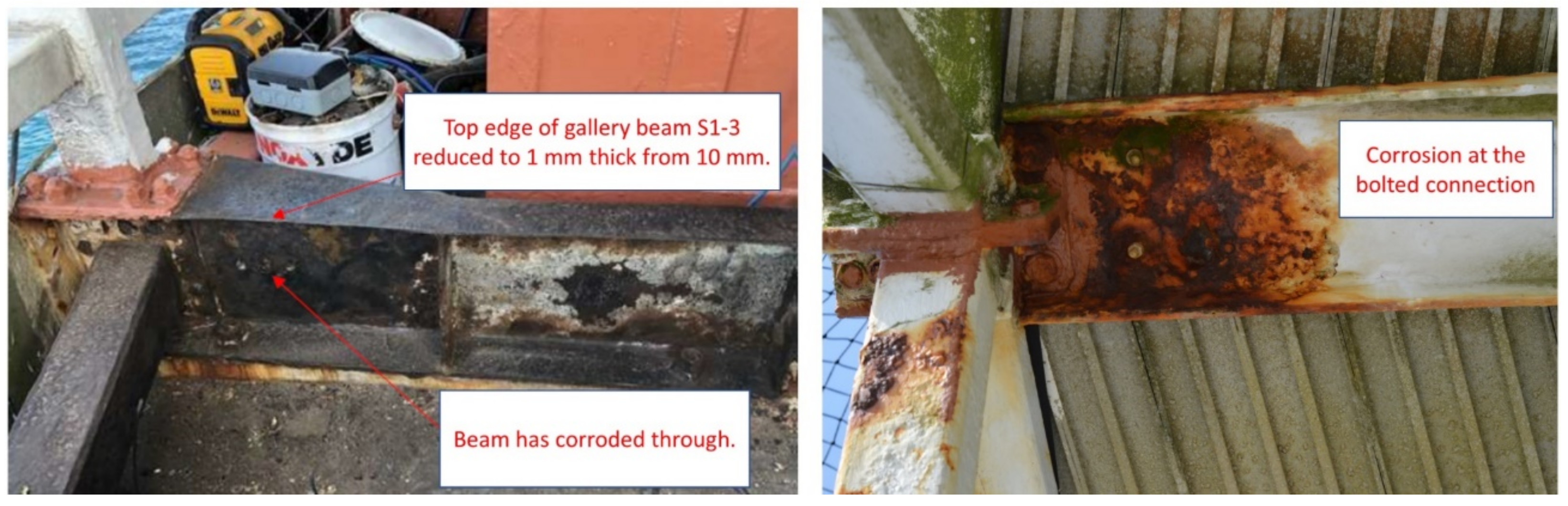
2.2. The Current Helideck Structure on the Bishop Rock Lighthouse
2.3. Extreme Value Analysis of Maximum Gust Speed
2.3.1. Data Homogenisation
2.3.2. Extreme Value Analysis Applied to the Homogenised Data
2.4. Extreme Wind Load Calculation
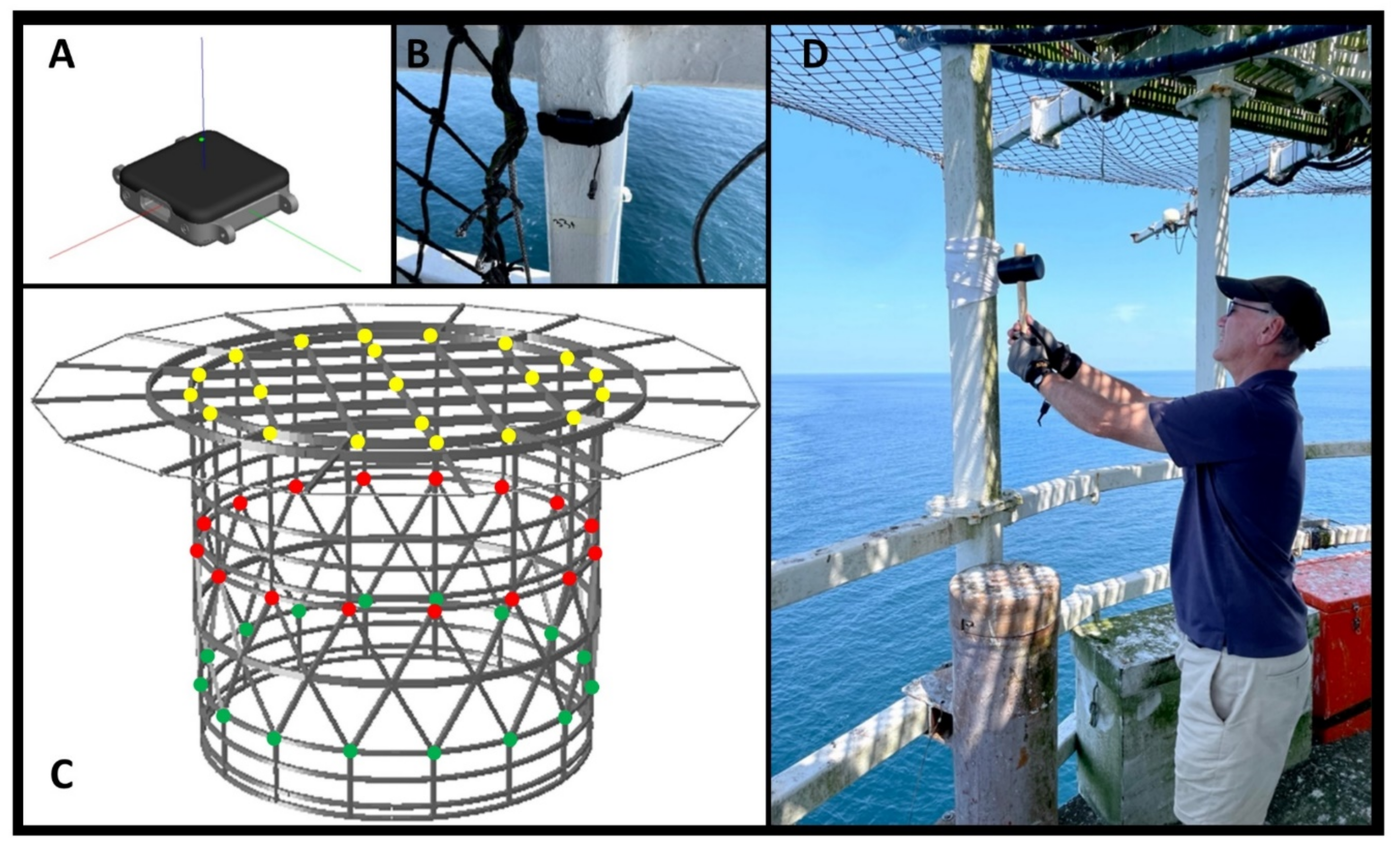
2.5. Modal Testing
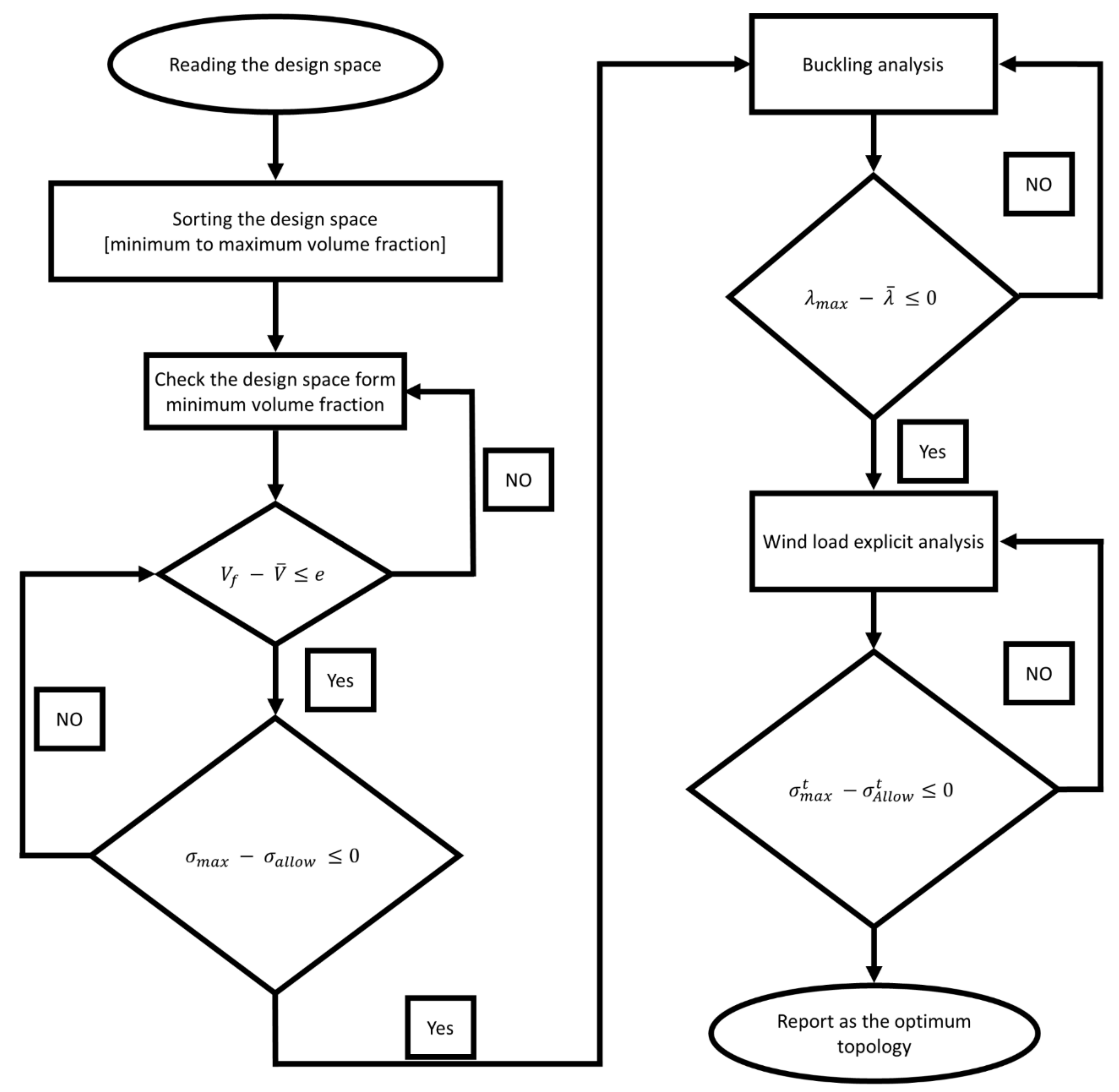
2.6. Design Computational Framework
2.6.1. Material
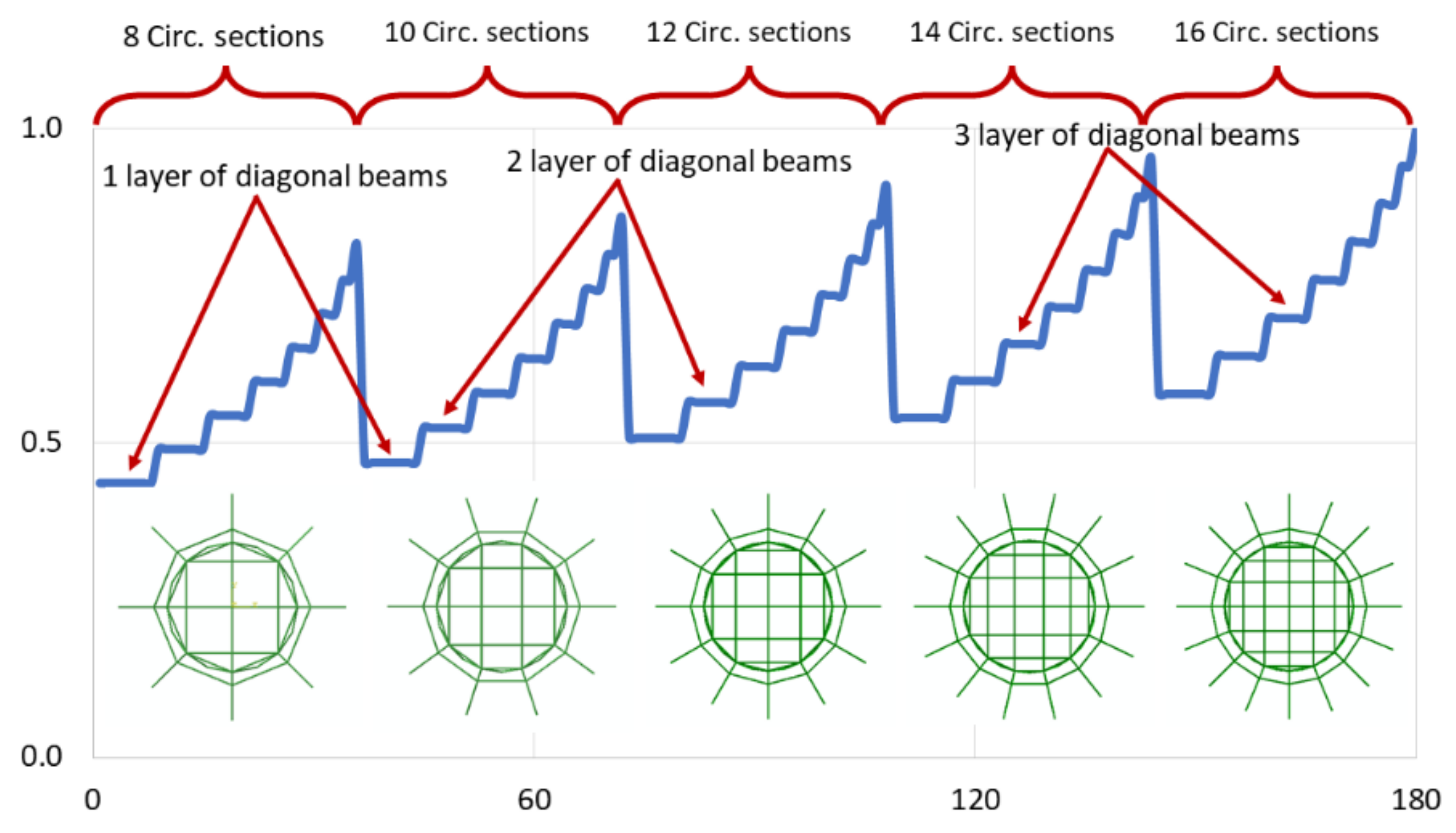
2.6.2. Exploring Different Topologies for the Lightest Helideck
- Helideck geometry:
- ➢
- Height of the helideck;
- ➢
- Diameter of the supporting structure;
- ➢
- Diameter of the landing deck;
- ➢
- Overall diameter of the helipad including the safety net beams;
- ➢
- Number of circumferential sections;
- ➢
- Number of vertical sections.
- The helicopter properties:
- ➢
- Total mass of the helicopter for which the helideck is designed;
- ➢
- Length of the skids of the helicopter;
- ➢
- Spacing between the helicopter skids.
- Wind load;
- Beams cross section.
2.6.3. Loads
- Dynamic load due to impact landing
- Sympathetic response of landing platform
- Overall superimposed load on the landing platform
- Lateral load on landing platform supports
- Dead load of structural members
- Wind loading

2.6.4. Buckling Analysis
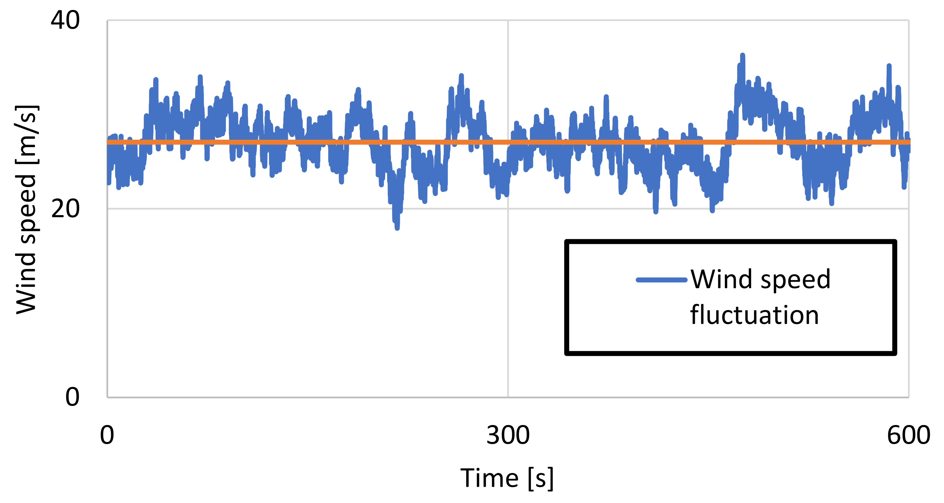
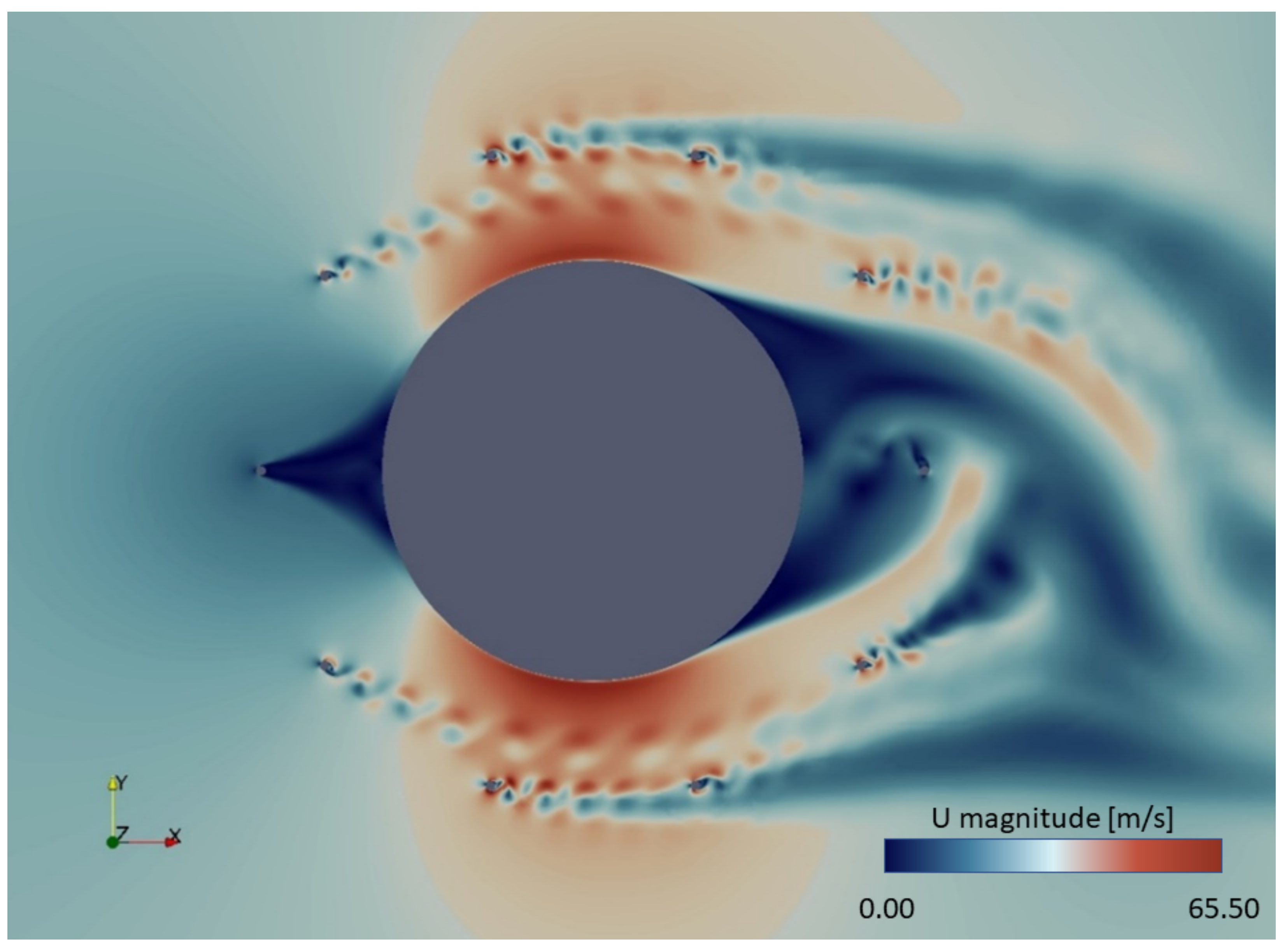
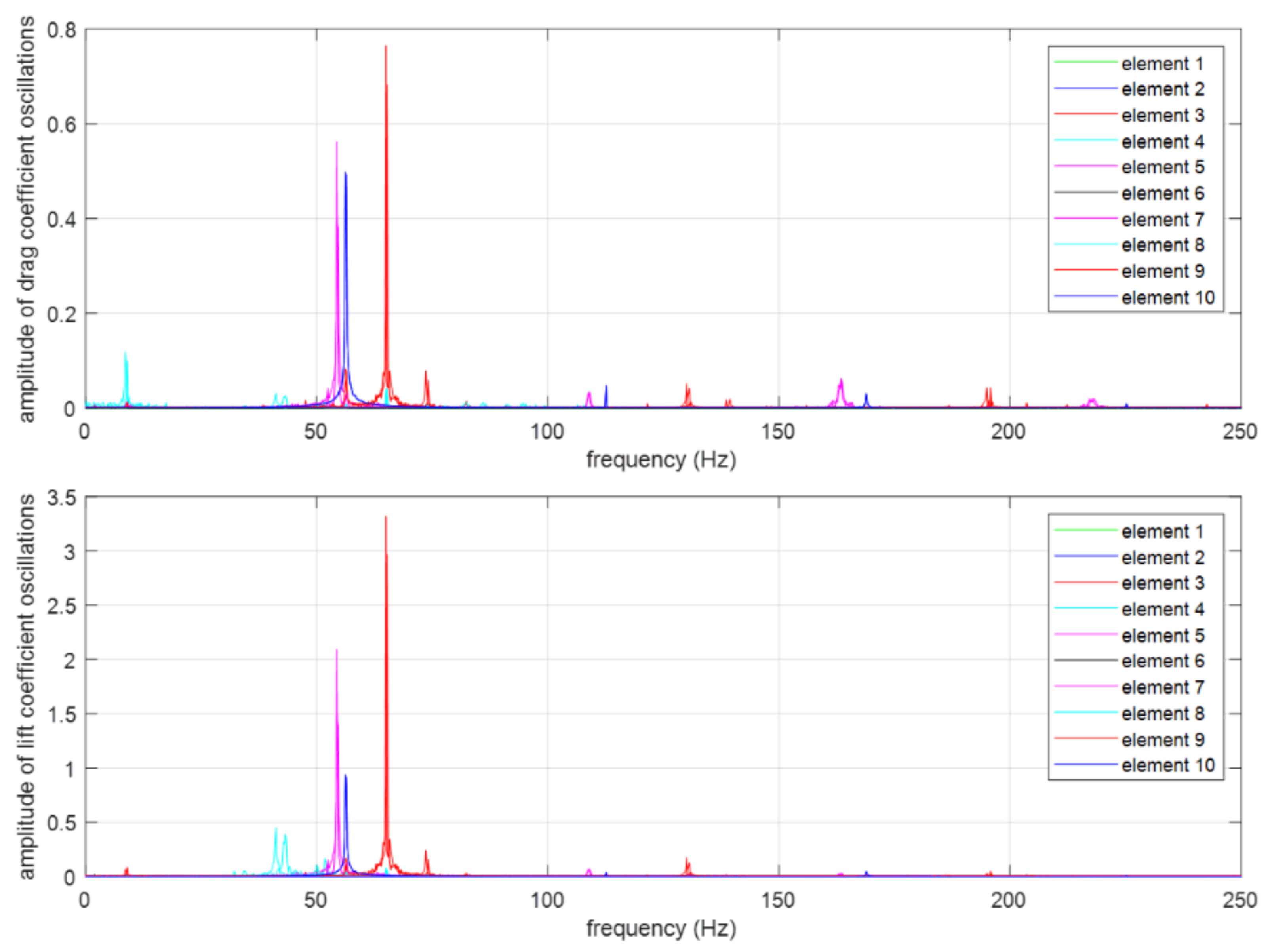
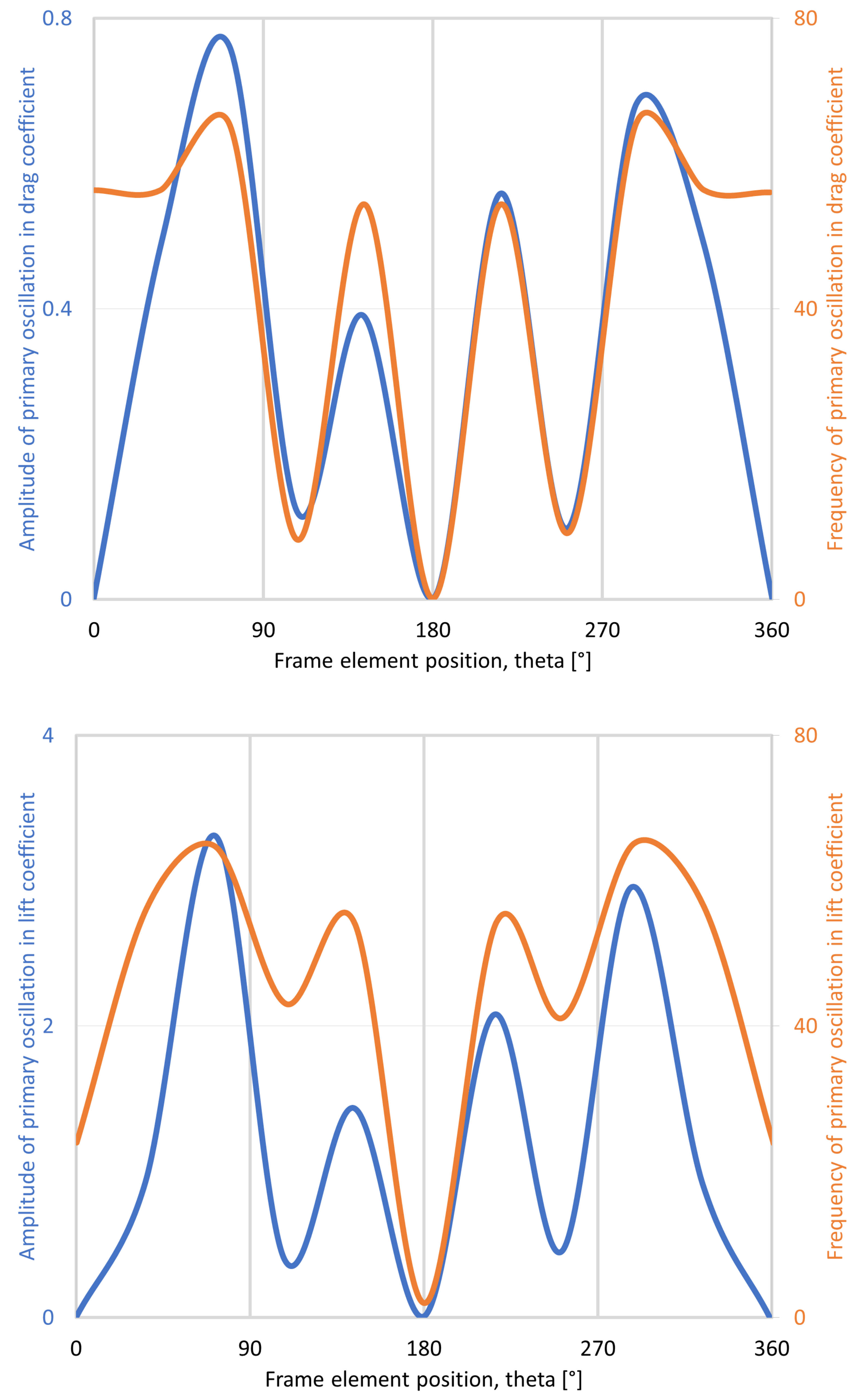
2.6.5. Dynamic Analysis of the Wind Loading
3. Results
3.1. Extreme Value Estimates of Gust Speed
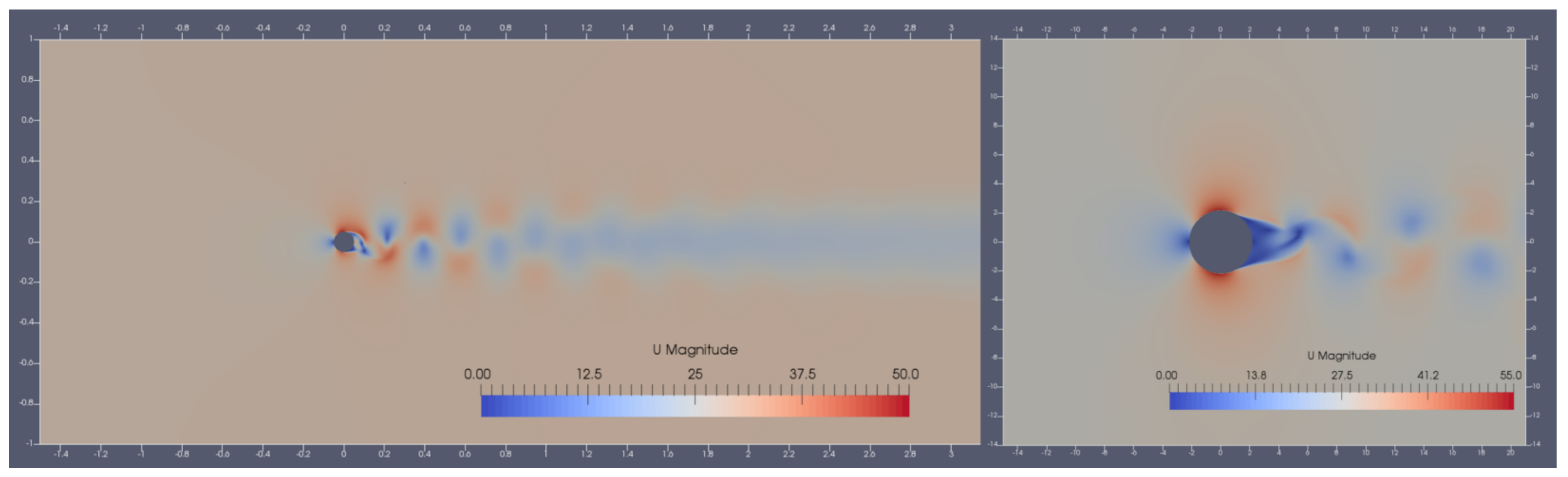
3.2. Wind Load on the Helideck as Function of Time and Location
3.3. Modal Analysis
3.4. The Optimum Helideck Structure
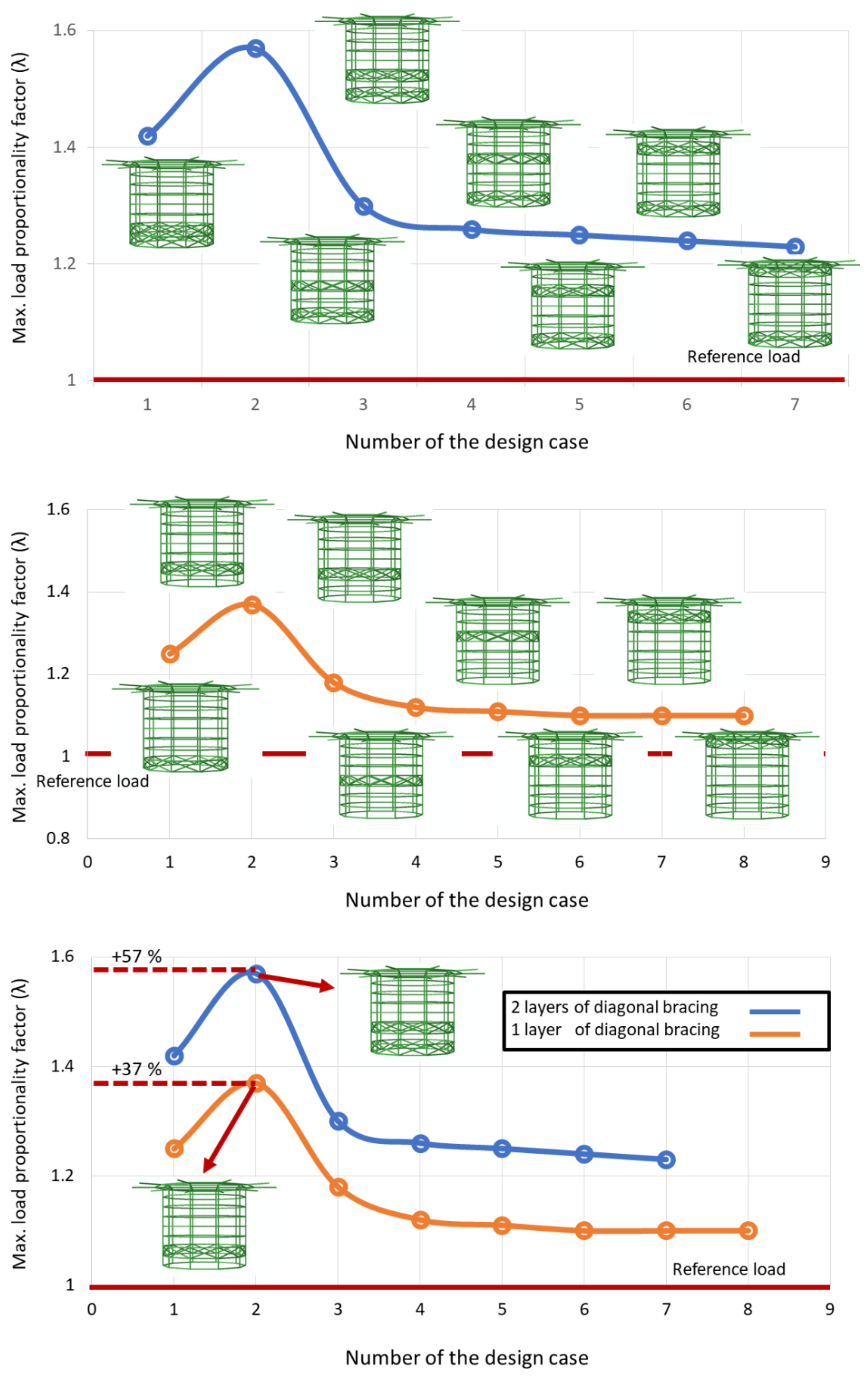
3.4.1. Buckling Analysis
3.4.2. Dynamic Analysis of the Wind Loading
4. Discussion
Author Contributions
Funding
Institutional Review Board Statement
Informed Consent Statement
Acknowledgments
Conflicts of Interest
References
- Raby, A.; Antonini, A.; D’Ayala, D.; Brownjohn, J.M.W. Environmental loading of heritage structures. Philos. Trans. R. Soc. A 2019, 377, 20190276. [Google Scholar] [CrossRef] [PubMed]
- Raby, A.C.; Antonini, A.; Pappas, A.; Dassanayake, D.T.; Brownjohn, J.M.W.; D’Ayala, D. Wolf Rock lighthouse: Past developments and future survivability under wave loading. Philos. Trans. R. Soc. A 2019, 377, 20190027. [Google Scholar] [CrossRef] [PubMed]
- Antonini, A.; Raby, A.; Brownjohn, J.M.W.; Pappas, A.; D’Ayala, D. Survivability assessment of fastnet lighthouse. Coast. Eng. 2019, 150, 18–38. [Google Scholar] [CrossRef]
- Brownjohn, J.M.W.; Raby, A.; Au, S.-K.; Zhu, Z.; Wang, X.; Antonini, A.; Pappas, A.; D’Ayala, D. Bayesian operational modal analysis of offshore rock lighthouses: Close modes, alignment, symmetry and uncertainty. Mech. Syst. Signal Process. 2019, 133, 106306. [Google Scholar] [CrossRef]
- Sigmund, O.; Maute, K. Topology optimization approaches: A comparative review. Struct. Multidiscip. Optim. 2013, 48, 1031–1055. [Google Scholar] [CrossRef]
- Ansys® Academic Research Mechanical, Release 2020, Help System, Mechanical Analysis Guide; ANSYS, Inc: Canonsburg, PA, USA, 2020.
- Michael, S. ABAQUS/Standard User’s Manual, Version 6.9; Dassault Systems: Vélizy-Villacoublay, France, 2009. [Google Scholar]
- Livermore Software Technology Corporation. LS-Dyna Keyword User’s Manual; Livermore Software Technology: Livermore, CA, USA, 2014. [Google Scholar]
- Maheri, A. Multiobjective optimisation and integrated design of wind turbine blades using WTBM-ANSYS for high fidelity structural analysis. Renew. Energy 2020, 145, 814–834. [Google Scholar] [CrossRef]
- Zhou, Y.; Tian, K.; Xu, S.; Wang, B. Two-scale buckling topology optimization for grid-stiffened cylindrical shells. Thin- Walled Struct. 2020, 151, 106725. [Google Scholar] [CrossRef]
- Yan, X.; Bao, D.; Zhou, Y.; Xie, Y.; Cui, T. Detail control strategies for topology optimization in architectural design and development. Front. Archit. Res. 2021, 11, 340–356. [Google Scholar] [CrossRef]
- Shanmugasundar, G.; Dharanidharan, M.; Vishwa, D.; Kumar, A.P.S. Design, analysis and topology optimization of connecting rod. Mater. Today Proc. 2021, 46, 3430–3438. [Google Scholar] [CrossRef]
- Tian, X.; Sun, X.; Liu, G.; Deng, W.; Wang, H.; Li, Z.; Li, D. Optimization design of the jacket support structure for offshore wind turbine using topology optimization method. Ocean Eng. 2022, 243, 110084. [Google Scholar] [CrossRef]
- Tsavdaridis, K.D.; Nicolaou, A.; Mistry, A.D.; Efthymiou, E. Topology optimisation of lattice telecommunication tower and performance-based design considering wind and ice loads. Structures 2020, 27, 2379–2399. [Google Scholar] [CrossRef]
- He, L.; Gilbert, M.; Shepherd, P.; Ye, J.; Koronaki, A. A new conceptual design optimization tool for frame structures. In Proceedings of the IASS Annual Symposium: Creativity in Structural Design, Boston, MA, USA, 16–20 July 2018; MIT: Cambridge, MA, USA, 2018. [Google Scholar]
- Ye, J.; Shepherd, P.; He, L.; Gilbert, M.; Davison, B.; Tyas, A.; Gondzio, J.; Weldeyesus, A.; Fairclough, H. Computational layout design optimization of frame structures. In Proceedings of the IASS Annual Symposium, Hamburg, Germany, 25–28 September 2017. [Google Scholar]
- Weldeyesus, A.G.; Gondzio, J.; He, L.; Gilbert, M.; Shepherd, P.; Tyas, A. Adaptive solution of truss layout optimization problems with global stability constraints. Struct. Multidiscip. Optim. 2019, 60, 2093–2111. [Google Scholar] [CrossRef]
- Dorn, W.; Gomory, R.; Greenberg, H.J. Automatic design of optimal structures. J. Mecanique 1964, 3, 25–52. [Google Scholar]
- Met Office. Dataset Collection Record: Met Office Integrated Data Archive System (MIDAS) Land and Marine Surface Stations Data (1853-Current); NCAS British Atmospheric Data Centre: Leeds, UK, 2021; Available online: catalogue.ceda.ac.uk (accessed on 10 December 2021).
- Martyn, S. MIDAS Data User Guide for UK Land Observations; v20210705, Documentation; Met Office: Exeter, UK, 2021; Available online: cedadocs.ceda.ac.uk/ (accessed on 9 December 2021).
- Turner, R.; Pirooz, A.A.S.; Flay, R.G.J.; Moore, S.; Revell, M. Use of High-Resolution Numerical Models and Statistical Approaches to Understand New Zealand Historical Wind Speed and Gust Climatologies. J. Appl. Meteorol. Climatol. 2019, 58, 1195–1218. [Google Scholar] [CrossRef]
- Miller, C.; Holmes, J.; Henderson, D.; Ginger, J.; Morrison, M. The Response of the Dines Anemometer to Gusts and Comparisons with Cup Anemometers. J. Atmos. Ocean. Technol. 2013, 30, 1320–1336. [Google Scholar] [CrossRef]
- Cook, J.N. The Designer’s Guide to Wind Loading of Building Structures. Part 1, Background, Damage Survey, Wind Data and Structural Classification; Butterworths: London, UK, 1985. [Google Scholar]
- Lienhard, J.H. Synopsis of Lift, Drag, and Vortex Frequency Data for Rigid Circular Cylinders; Bulletin 300; Technical Extension Service, Washington State University: Washington, DC, USA, 1966. [Google Scholar]
- White, F.M. Fluid Mechanics, 5th ed.; McGraw-Hill: New York, NY, USA, 2003. [Google Scholar]
- EEN 1999-1-1; Eurocode 9: Design of Aluminium Structures—Part 1-1: General Structural Rules. The European Union Per Regulation 305/2011, Directive 98/34/EC, Directive 2004/18/EC; ICE Publishing: London, UK, 2007.
- Majzoobi, G.H.; Freshteh-Saniee, F.; Khosroshahi, S.F.Z.; Mohammadloo, H.B. Determination of materials parameters under dynamic loading. Part I: Experiments and simulations. Comput. Mater. Sci. 2010, 49, 192–200. [Google Scholar] [CrossRef]
- Wei, P.; Liu, Y.; Dai, J.G.; Li, Z.; Xu, Y. Structural design for modular integrated construction with parameterized level set-based topology optimization method. Structures 2021, 31, 1265–1277. [Google Scholar] [CrossRef]
- Teimouri, M.; Mahbod, M.; Asgari, M. Topology-optimized hybrid solid-lattice structures for efficient mechanical performance. Structures 2021, 29, 549–560. [Google Scholar] [CrossRef]
- Xiao, M.; Mukherjee, S.; Raghavan, B.; Dutta, S.; Breitkopf, P.; Zhang, W. Revisiting p-refinement in structural topology optimization. Structures 2021, 34, 3640–3646. [Google Scholar] [CrossRef]
- Luo, Z.; Yang, J.; Chen, L. A new procedure for aerodynamic missile designs using topological optimization approach of continuum structures. Aerosp. Sci. Technol. 2006, 10, 364–373. [Google Scholar] [CrossRef]
- Youn, S.K.; Park, S.H. A study on the shape extraction process in the structural topology optimization using homogenized material. Comput. Struct. 1997, 62, 527–538. [Google Scholar] [CrossRef]
- Yang, R.J.; Chuang, C.H. Optimal topology design using linear programming. Comput. Struct. 1994, 52, 265–275. [Google Scholar] [CrossRef]
- Martin, A.; Deierlein, G.G. Structural topology optimization of tall buildings for dynamic seismic excitation using modal decomposition. Eng. Struct. 2020, 216, 110717. [Google Scholar] [CrossRef]
- CAP 437; Standards for Offshore Helicopter Landing Areas. Civil Aviation Authority: London, UK, 2021.
- Riks, E. The Application of Newton’s Method to the Problem of Elastic Stability. J. Appl. Mech. 1972, 39, 1060–1065. [Google Scholar] [CrossRef]
- Zhao, Y.; Zhai, X.; Wang, J. Buckling behaviors and ultimate strengths of 6082-T6 aluminum alloy columns under eccentric compression—Part I: Experiments and finite element modeling. Thin-Walled Struct. 2019, 143, 106207. [Google Scholar] [CrossRef]
- Riks, E. An incremental approach to the solution of snapping and buckling problems. Int. J. Solids Struct. 1979, 15, 529–551. [Google Scholar] [CrossRef]
- Kwon, D.; Kareem, A. NatHaz On-Line Wind Simulator (NOWS): Simulation of Gaussian Multivariate Wind Fields. NatHaz Modeling Laboratory Report. 2006. Available online: windsim.ce.nd.edu/ (accessed on 20 December 2021).
- Kwon, D.K.; Kareem, A. A framework for gust-front factor in Conference. In Proceedings of the 11th Americas Conference on Wind Engineering (ACWE 11), San Juan, Puerto Rico, 22–26 June 2009. [Google Scholar]
- Juang, J.N.; Pappa, R.S. An eigensystem realization algorithm for modal parameter identification and model reduction. J. Guid. Control. Dyn. 2012, 8, 620–627. [Google Scholar] [CrossRef]
- Ottersböck, M.J.; Leitner, M.; Stoschka, M. Characterisation of actual weld geometry and stress concentration of butt welds exhibiting local undercuts. Eng. Struct. 2021, 240, 112266. [Google Scholar] [CrossRef]
- Pandey, M.; Young, B. Experimental investigation on stress concentration factors of cold-formed high strength steel tubular X-joints. Eng. Struct. 2021, 243, 112408. [Google Scholar] [CrossRef]
- Feng, R.; Tang, C.; Chen, Z.; Roy, K.; Chen, B.; Lim, J.B.P. A numerical study and proposed design rules for stress concentration factors of stainless steel hybrid tubular K-joints. Eng. Struct. 2021, 233, 111916. [Google Scholar] [CrossRef]
- Godio, M.; Portal, N.W.; Flansbjer, M.; Magnusson, J.; Byggnevi, M. Experimental and numerical approaches to investigate the out-of-plane response of unreinforced masonry walls subjected to free far-field blasts. Eng. Struct. 2021, 239, 112328. [Google Scholar] [CrossRef]
- Aursand, E.; Dumoulin, S.; Hammer, M.; Lange, H.I.; Morin, A.; Munkejord, S.T.; Nordhagen, H.O. Fracture propagation control in CO2 pipelines: Validation of a coupled fluid-structure model. Eng. Struct. 2016, 123, 192–212. [Google Scholar] [CrossRef]
- Bergmeister, K.; Brunello, P.; Pachera, M.; Pesavento, F.A. Schrefler, Simulation of fire and structural response in the Brenner Base Tunnel by means of a combined approach: A case study. Eng. Struct. 2020, 211, 110319. [Google Scholar] [CrossRef]


| Element | Mesh | dx (m) | dy (m) | Δs (m) | No. Layers | Layer Expansion Ratio | Total Number of Cells | Δt |
|---|---|---|---|---|---|---|---|---|
| frame | 1 | 0.080 | 0.086 | 0.001 | 4 | 2 | 5233 | 0.00018 |
| frame | 2 | 0.040 | 0.046 | 0.001 | 4 | 1.6 | 17,851 | 0.00011 |
| frame | 3 | 0.020 | 0.024 | 0.001 | 3 | 1.6 | 62,579 | 0.00005 |
| frame | 4 | 0.013 | 0.016 | 0.001 | 2 | 1.6 | 139,111 | 0.000333 |
| lantern | 0 | 0.159 | 0.171 | 0.0014 | 4 | 1.8 | 68,847 | 0.00025 |
| lantern | 1 | 0.080 | 0.085 | 0.0014 | 4 | 1.8 | 263,738 | 0.00018 |
| lantern | 2 | 0.040 | 0.043 | 0.0014 | 3 | 1.8 | 1,013,048 | 0.000125 |
| Material | Type of Analysis | Constitutive Material Model | Elastic Modulus | Poisson’s Ratio | Yield Stress |
|---|---|---|---|---|---|
| Steel | Modal | Elastic | 200 GPa | 0.3 | --- |
| Aluminium | Static | Elastic | 70 GPa | 0.3 | --- |
| Aluminium | Riks | Elastic-Perfect plastic | 70 GPa | 0.3 | 125 MPa |
| Aluminium | Explicit | Elastic | 70 GPa | 0.3 | --- |
| TR (Years) | 3 s Gust Speed (m/s) | 10 min Mean Wind Velocity (m/s) |
|---|---|---|
| 2 | 31.2 [30.6;32.0] | 21.6 [21.2;22.2] |
| 10 | 34.6 [33.4;36.7] | 23.9 [23.1;25.4] |
| 20 | 36.0 [34.5;39.1] | 24.9 [23.9;27.1] |
| 50 | 37.8 [35.8;42.8] | 26.2 [24.8;29.7] |
| 100 | 39.1 [36.7;46.0] | 27.1 [25.4;31.9] |
| 150 | 39.8 [37.2;48.1] | 27.6 [25.8;33.3] |
| 200 | 40.3 [37.5;49.6] | 28.0 [26.0;34.3] |
| 250 | 40.8 [37.8;50.8] | 28.2 [26.2;35.2] |
| Mode 1 | Mode 2 | Mode 3 | |||
|---|---|---|---|---|---|
| Num.: 4.30 Hz | Exp.: 4.05 Hz | Num.: 4.30 Hz | Exp.: 4.09 Hz | Num.: 4.68 Hz | Exp.: 5.03 Hz |
 |  |  |  |  |  |
 |  |  |  |  |  |
 |  |  |  |  |  |
| Static Analysis | ||
| Volume fraction | 44% | 46% |
| Maximum stress | 54 MPa | 44 MPa |
| Von_Mises stress distribution | 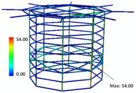 |  |
| Riks Analysis | ||
| 37% | 47% | |
| Dynamic (Time-Dependent) Analysis | ||
| Average stress | 56.3 MPa | 55.8 MPa |
| Maximum stress | 111.8 MPa (at 1790 s) | 111.6 MPa (at 1440 s) |
| Von_Mises stress distribution | 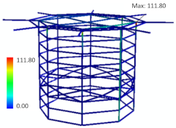 | 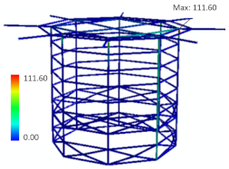 |
Publisher’s Note: MDPI stays neutral with regard to jurisdictional claims in published maps and institutional affiliations. |
© 2022 by the authors. Licensee MDPI, Basel, Switzerland. This article is an open access article distributed under the terms and conditions of the Creative Commons Attribution (CC BY) license (https://creativecommons.org/licenses/by/4.0/).
Share and Cite
Khosroshahi, S.F.; Masina, M.; Antonini, A.; Ransley, E.; Brownjohn, J.M.W.; Dobson, P.; D’Ayala, D. A Multidisciplinary Computational Framework for Topology Optimisation of Offshore Helidecks. J. Mar. Sci. Eng. 2022, 10, 1180. https://doi.org/10.3390/jmse10091180
Khosroshahi SF, Masina M, Antonini A, Ransley E, Brownjohn JMW, Dobson P, D’Ayala D. A Multidisciplinary Computational Framework for Topology Optimisation of Offshore Helidecks. Journal of Marine Science and Engineering. 2022; 10(9):1180. https://doi.org/10.3390/jmse10091180
Chicago/Turabian StyleKhosroshahi, Siamak Farajzadeh, Marinella Masina, Alessandro Antonini, Edward Ransley, James Mark William Brownjohn, Peter Dobson, and Dina D’Ayala. 2022. "A Multidisciplinary Computational Framework for Topology Optimisation of Offshore Helidecks" Journal of Marine Science and Engineering 10, no. 9: 1180. https://doi.org/10.3390/jmse10091180
APA StyleKhosroshahi, S. F., Masina, M., Antonini, A., Ransley, E., Brownjohn, J. M. W., Dobson, P., & D’Ayala, D. (2022). A Multidisciplinary Computational Framework for Topology Optimisation of Offshore Helidecks. Journal of Marine Science and Engineering, 10(9), 1180. https://doi.org/10.3390/jmse10091180