A Novel Underwater Image Enhancement Algorithm and an Improved Underwater Biological Detection Pipeline

Abstract

For aquaculture resource evaluation and ecological environment monitoring, the automatic detection and identification of marine organisms is critical; however, due to the low quality of underwater images and the characteristics of underwater biological detection, the lack of abundant features can impede traditional hand-designed feature extraction approaches or CNN-based object detection algorithms, particularly in complex underwater environments. Therefore, the goal of this study was to perform object detection in underwater environments. This study developed a novel method for capturing feature information by adding the convolutional block attention module (CBAM) to the YOLOv5 backbone network. The interference of underwater organism characteristics in object characteristics decreased and the output object information of the backbone network was enhanced. In addition, a self-adaptive global histogram stretching algorithm (SAGHS) was designed to eliminate degradation problems, such as low contrast and color loss, that are caused by underwater environmental features in order to restore image quality. Extensive experiments and comprehensive evaluations using the URPC2021 benchmark dataset demonstrated the effectiveness and adaptivity of the proposed methods. Additionally, this study conducted an exhaustive analysis of the impacts of training data on performance.

1. Introduction

The exploration of aquatic environments has recently become popular due to the growing scarcity of natural resources and the growth of the global economy [1]. Machine vision has been shown to be a low-cost and dependable method that has the benefits of non-contact monitoring, long-term steady operation, and a broad range of applications. Underwater object detection is pivotal in numerous applications, such as underwater search and rescue operations, deep-sea exploration and archaeology, and sea life monitoring [2]. These applications require effective and precise vision-based underwater sea analytics, including image enhancement, image quality assessment, and object detection methods. However, capturing underwater images using optical imaging systems poses greater problems than capturing images under open-air conditions. More specifically, underwater images frequently suffer from degeneration due to severe color distortion, low contrast, non-uniform illumination, and noise from artificial lighting sources, which dramatically degrades image visibility and affects the detection accuracy for underwater object detection tasks [1]. Over recent years, underwater image enhancement technologies have been developed that work as preprocessing operations to boost detection accuracy by improving the visual quality of underwater images.

On the other hand, underwater object detection performance is associated with the characteristics of underwater biological organisms. Usually, because of differences in size or shape and the overlapping or occlusion of marine organisms, traditional hand-designed feature extraction methods cannot meet detection requirements for actual underwater scenes. Most studies have emphasized the extraction of traditional low-level features, such as color, texture, contours, and shape [3], which has led to the disadvantages of traditional object detection methods, such as poor recognition, low accuracy, and slow recognition. However, by directly benefiting from deep learning methods, object detection has witnessed a great boost in performance over recent years, although general object detection algorithms that are based on deep learning have not yet demonstrated better detection performance for marine organisms due to the low quality of underwater imaging and complex underwater environments.

The majority of the extant strategies consider underwater image enhancement and underwater object detection as two separate pipelines, with underwater image enhancement being evaluated by image quality assessments and underwater object detection being evaluated by detection accuracy. These two tasks have different optimization objectives, which lead to different optimal solutions.

To validate the proposed methods, this study conducted experiments using the underwater robot professional contest (URPC2021) dataset. The experimental results proved the effectiveness of the proposed underwater image enhancement method and the improved underwater object detection algorithm. In conclusion, the primary contributions of this study can be summarized as follows:

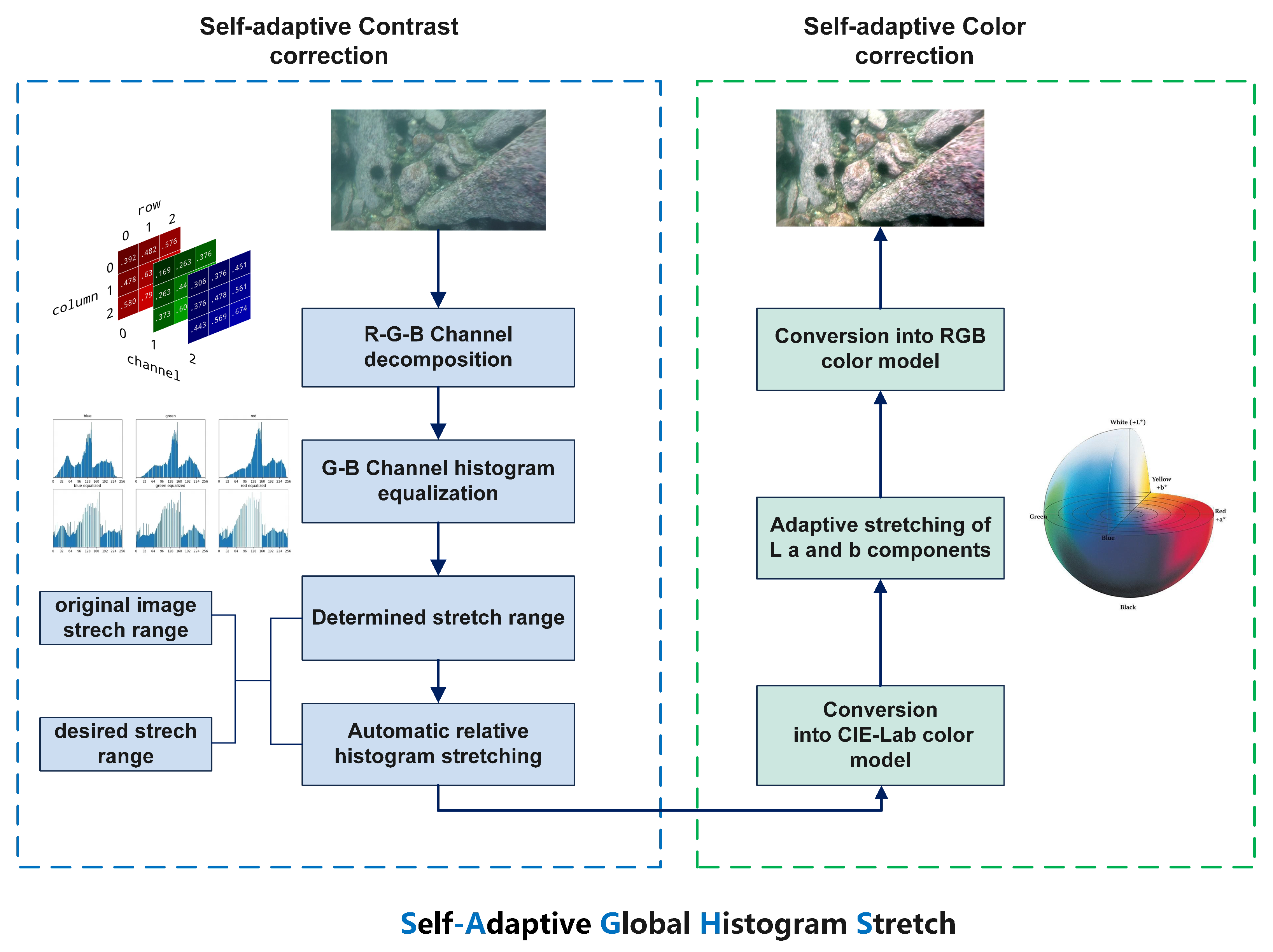
• The correction of bluish and greenish backgrounds and low contrast using an improved global histogram stretching method that dynamically adjusts the histogram stretching coefficient, for which a detailed linear function and framework were built;
• The integration of a convolutional block attention module (CBAM) into CSPDarknet53 to enhance the features of small, overlapping, and occluded objects. In particular, the CBAM mechanism can be employed to improve the contrast between an object and the surrounding environment and refine redundant information that is produced by the Focus function;
• The use of a simple and efficient connection between the attention mechanism and object detection algorithm for the first time. The CBAM module was added to the Focus module of the backbone network to reduce the model burden as much as possible while ensuring the desired detection accuracy of the improved algorithm.

The rest of the paper is organized as follows. Related works are discussed in Section 2. Section 3 describes the materials and methods that were used in this study, including details about the detection algorithm for the improved YOLOv5. In Section 4, the experiments and performance analysis on the improved underwater model are presented. Finally, the conclusions are presented in Section 5.

2. Related Work

2.1. Underwater Image Enhancement (UIE) Methods

Underwater image enhancement (UIE) is a necessary step to improve the visual quality of underwater images. UIE can be divided into three categories: model-free, physical model-based, and deep learning-based approaches.

White balance [4], Gray World theory [5], and histogram equalization [6] are examples of model-free enhancement methods that improve the visual quality of underwater images by directly adjusting the pixel values of images. Ancuti et al. suggested a multi-scale fusion underwater image enhancement method that could be combined with fusion color correction and contrast enhancement to obtain high-quality images [7]. Based on prior research, Ancuti et al. also proposed a weighted multi-scale fusion method for underwater image white balance that could restore faded information and edge information in the original images using gamma variation and sharpening [8]. Fu et al. proposed a Retinex-based enhancement system that included color correction, layer decomposition, and underwater image enhancement in the Lab color space [9]. Zhang et al. extended the Retinex-based method by using bilateral and trilateral filters to enhance the three channels of underwater image in the CIELAB color space [10]. However, because the physical deterioration process of underwater images has not been taken into account, the model-free UIE approaches can generate noise, artifacts, and color distortion, which makes them unsuitable for various types of applications.

Physical model-based methods regard underwater picture enhancement as an inverse image degradation problem and these algorithms can provide clear images by calculating the transmission and background light using Definition 1. Because underwater imaging models are similar to atmospheric models for fog, dehazing algorithms are used to enhance underwater images. He et al. proposed a dehazing algorithm that was based on dark channel prior (DCP), which could effectively estimate the thickness of fog and obtain fog-free images [11]. Based on DCP, Drew et al. proposed an underwater dark channel prior that considered red light attenuation in water [12]. Peng et al. developed a generalized dark primary color prior (GDCP) for underwater image enhancement that included adaptive color correction in an image creation model [13]. Model-based approaches often need prior information and the quality of the improved images is dependent on precise parameter estimation.

Deep learning enhancement methods usually construct convolutional neural networks and train them using pairs of degraded underwater images and their high-quality counterparts [14]. Li et al. suggested an unsupervised generative adversance network (WaterGAN) that generated underwater images from aerial RGB-D images and then trained an underwater image recovery network using the synthesized training data [15]. To produce paired underwater image datasets, Fabbri et al. suggested an underwater color transfer model that was based on CycleGAN [16] and built an underwater image recovery network using a gradient penalty technique [17]. Ye et al. proposed an unsupervised adaptive network for joint learning that could jointly estimate scene depth and correct color underwater images [18]. Chen et al. proposed two perceptual enhancement cascade models, which used gradient strategy feedback information to enhance more prominent features in images [14]. Deep learning UIE approaches that are based on composite image training generally require a large number of datasets [19]. Because the quality of the composite images cannot be guaranteed, these methods cannot be applied to underwater situations.

2.2. Attention Mechanisms

Some studies on attention mechanisms have been presented in the literature. Attention models enable networks to extract information from crucial areas with reduced energy consumption, thereby enhancing CNN performance. Wang et al. proposed a residual attention network that was based on an attention mechanism, which could continuously extract large amounts of attention information [20]. Hu et al. proposed SENet, which contained architectural “squeeze” and “excitation” units. These modules enhanced network expressiveness by modeling the interdependencies between channels [21]. Woo et al. proposed a lightweight module (CBAM) that combined feature channels and feature spaces to refine features [22]. This method could achieve considerable performance improvements while maintaining small overheads.

2.3. Underwater Object Detection Algorithms

Deep learning-based object detection algorithms are currently divided into two categories: one-stage regression detectors and two-stage region generation detectors. One-stage detection methods mainly include the YOLO series [23,24,25], SSDs [26], RetinaNet [27], and RefineDet [28], which directly predict objects without region generation. Two-stage detection methods mainly include RCNNs [29], fast RCNNs [30], faster RCNNs [31], and cascade RCNNs [32]. Initially, these object detection methods were used for natural environments on land. As deep learning technology has advanced, more and more object detection algorithms have been applied to challenging underwater environments. Li et al. used a faster RCNN to detect fish species and achieved an outstanding performance [33]. Li et al. employed a residual network to detect deep-sea plankton. Their experiments revealed that deep residual networks generalized plankton categorization [34]. Cui et al. introduced a CNN-based fish detection system and optimized it using data augmentation, network simplification, and training process acceleration [35]. Huang et al. presented three data augmentation approaches for underwater imaging that could imitate the illumination of marine environments [36]. Fan et al. suggested a cascade underwater detection framework with feature augmentation and anchoring refinement, which could address the issue of imbalanced underwater samples [37]. Zhao et al. designed a new composite backbone network to detect fish species by improving the residual network and used it to learn change information within ocean scenes [3]. However, little research has been conducted in the field of underwater object detection using YOLO.

The above section analyzed the existing research on underwater image enhancement, attention mechanisms, and one-stage object detection algorithms. According to the above analysis, object detection algorithms for terrestrial environments can be migrated and applied to underwater conditions. However, complex underwater environments and underwater biological properties can lead to low detection accuracy. In response to this problem, this study developed an improved UIE method and an improved YOLOv5 object detection algorithm to handle the degradation of underwater images and the low detection accuracy of existing methods in complex underwater environments.

3. Methodology

This section first presents an overview of the self-adaptive global histogram stretching algorithm (SAGHS) framework. Then, we demonstrate how to overcome underwater biological characteristics using the convolutional block attention module (CBAM). Next, the novel connection between the CBAM and the backbone network is outlined, followed by the training and inference. The algorithm is presented in detail in the following two subsections.

3.1. Self-Adaptive Histogram Stretching Algorithm

Due to the complexity of underwater environments, underwater images often contain visual distortions, such as low contrast, color distortions, and foggy effects. Before performing computer vision tasks, it is usual to consider image enhancement preprocessing methods. Using image enhancement methods, image quality can be improved and the use of high-quality images facilitates object detection. The main motivation and guidelines for designing the network architecture of the proposed framework are addressed as follows. In this section, a two-stage self-adaptive global histogram stretching algorithm (SAGHS) is introduced, which was based on the structure decomposition and characteristics of underwater imaging, as shown in Figure 1. It included a self-adaptive contrast correction module and a self-adaptive color correction module. In the self-adaptive contrast correction module, the first step was to decompose the RGB channels and then apply color equalization and SAGHS to adjust the dynamic stretching range. In addition, a bilateral was used to eliminate noise. In the self-adaptive color correction module, RGB images were converted into a CIELAB model and then a simple linear histogram stretching was applied to adjust the “L” component. The adjusted CIELAB model was finally converted back into an RGB model. The basic principles and definition were as follows.

Definition 1.

Simplified underwater optical imaging model (J-M model):

$$I^C(x,y)=J^C(x,y)t^C(x,y)+B^C(1-t^C(x,y))$$

(1)

where $C\in \{R,G,B\}$. $I^C(x,y)$ represents the underwater image that was captured by the camera, $J^C(x,y)t^C(x,y)$ represents the part of the scene energy that decayed directly, $J^C(x,y)$ represents the scene radiance, $t^C(x,y)$ represents the transmission map, and $B^C(x,y)$ represents the global background light. In water, $t^C(x,y)$ could be expressed as $e^{-\eta d(x,y)}$, where η is the attenuation coefficient and $d(x,y)$ is the depth map between the scene and the camera.

Definition 2.

Histogram stretching method (Iqbal):

$$P_o=(P_i-c)\frac{(b-c)}{(a-c)}+a$$

(2)

where $P_i$ and $P_o$ represent the input and output pixel values, respectively, a and b represent the minimum and maximum values of the desired range, respectively, and $c,d$ represents the lowest and highest pixel values that were present in the underwater images, respectively.

Definition 3.

The statistics of the histogram distribution with a large of underwater images showed that the distribution satisfied the Rayleigh distribution and its probability expression was obtained as:

$$RD=\frac{x}{a^2}{e}^{\frac{-x^2}{2a^2}}$$

(3)

where the scale parameter a of the distribution function is the mode, which represents the peak value in each RGB histogram. When a channel presented a normal distribution, the median and mode were the same value.

3.1.1. Self-Adaptive Contrast Correction Module

Raw underwater images have low contrast and indistinct details due to light attenuation and dispersion. To properly adjust the contrast and increase detail in these images, the first step was to decompose the RGB channels and then conduct color equalization. Our method for decomposing underwater images was inspired by the theory of the Gray World hypothesis: for an ideal image, the average of the RGB channels in the image should be “gray” (K). Because red light attenuation in water is difficult to adjust using simple color equalization, this process leads to the over-saturation of red light; so, according to the Gray World theory, half of the maximum values of the G and B channels were selected to take K = 0.5 as the "gray" value to correct those channels. Next, the image channels were dynamically adjusted using the self-adaptive histogram stretching method. The specific function of the dynamic adaptive stretching is documented in Algorithm 1.

Algorithm 1 The self-adaptive global histogram stretching algorithm.

Input:  original stretch range $I_{min}$, $I_{max}$, desired stretch range $O_{min}$, $O_{max}$, channel representation $\lambda$ Output:  Desired stretch minimum dynamic factor ${\beta }_{\lambda }$, Desired stretch maximum dynamic coefficient ${\mu }_{\lambda }$ 1: Begin 2: function stretchingRange($I_{min}$, $I_{max}$,$O_{min}$, $O_{max}$) 3: for$i,j\in [height,weight]$do 3:  initialize sort array 4: end for 5: $I_{min},I_{max}$ is the pixel values of the 0.5% and 99.5% array respectively 6: $O_{min}\in (0,I_{\lambda min})$ 7: $O_{min}=a_{\lambda }-{\beta }_{\lambda }\times {\sigma }_{\lambda }$ 8: $O_{max}\in (I_{\lambda max},255)$ 9: $O_{max}=I_{\lambda max}÷t_{\lambda }$ 10: $I_{max}=a_{\lambda }+{\mu }_{\lambda }\times {\sigma }_{\lambda }$ 11: end function 12: function stretching(${\beta }_{\lambda }$,${\mu }_{\lambda }$) 13: Discuss the solution of ${\beta }_{\lambda }$,${\mu }_{\lambda }$ to determine the stretch range and get the output pixel value $P_{out}$ 14: $P_{out}=(P_{in}-I_{min})\frac{(O_{max}-O_{min})}{(I_{max}-I_{min})}+O_{min}$ 15: return$P_{out}$

This excessive stretching of certain color channels not only introduced noise that reduced the visibility of the images but it also introduced artifacts that caused color distortion and corrupted the details of the original images. According to the distribution patterns of the RGB histograms of underwater images, the global histogram stretching equation (Definition 2) was rewritten as Equation (4):

$$P_{out}=(P_{in}-I_{min})\frac{(O_{max}-O_{min})}{(I_{max}-I_{min})}+O_{min}$$

(4)

where $P_{in}$ and $P_{out}$ represent the input and output pixel values, respectively, and $I_{min},I_{max},$$O_{min},O_{max}$ represent the adaptive parameters of the images before and after stretching, respectively.

Selection of stretching range $I_{min},I_{max}$: Generally, this stretching process was configured to follow the Rayleigh distribution (Definition 3) and was restricted to a specific range. However, to reduce the effects of stretching due to extreme pixel points (e.g., noise, maxima, minima, etc.) in the underwater images, the upper and lower intensity values were separated. In the proposed methods, the input intensity levels were limited to 5% of the minimum and maximum limitations. The restrictions were used to mitigate the effects of under- and over-exposure in underwater images, as shown by Equation (5):

$$\left\{\begin{array}{c}{I}_{min}={\sigma }_{st}[{\sigma }_{st.index}\left(a\right)\times 0.5\%]\hfill \\ I_{max}={\sigma }_{st}[-({\sigma }_{len}-{\sigma }_{st.index}\left(a\right))\times 0.5\%]\hfill \end{array}\right.$$

(5)

where $I_{min}$ and $I_{max}$ represent the minimum and maximum stretch values, respectively, ${\sigma }_{st}$ represents the ascending arrangement of the pixels in each RGB channel, ${\sigma }_{st.index}\left(a\right)$ represents the index of the distribution pattern of the histogram, ${\sigma }_{len}$ represents the size of the image, and ${\sigma }_{st}[·]$ represents the value of the index of the forward arraying pixel set.

Selection of the desired range $O_{min},O_{max}$:The global histogram stretching algorithm expected the stretching range to be [0, 255], which resulted in excessive blue-green illumination in the underwater images. A simplified minimum desired stretching range was obtained by calculating the standard deviation of the Rayleigh distribution:

$$O_{min}=a_{\lambda }-{\beta }_{\lambda }\times {\sigma }_{\lambda }$$

(6)

where $a_{\lambda }$ is the mode of the channel, ${\beta }_{\lambda }$ is the dynamic minimum tensile coefficient, ${\sigma }_{\lambda }$ is the standard deviation of the Rayleigh distribution, and ${\sigma }_{\lambda }=0.655a_{\lambda }$.

Next, the maximum desired stretch was determined based on the underwater imaging model (Definition 1) and the different attenuation levels that were exhibited by the light as it propagated through the water.

$$O_{max}=\frac{I_{\lambda }}{\kappa \times t_{\lambda }}=\frac{a_{\lambda }+{\mu }_{\lambda }\times {\sigma }_{\lambda }}{\kappa \times t_{\lambda }}$$

(7)

The coefficient ${\mu }_{\lambda }$ was satisfied:

$$\frac{\kappa \times t_{\lambda }\times I_{\lambda }}{{\sigma }_{\lambda }}\le {\mu }_{\lambda }+1.526\le \frac{\kappa \times t_{\lambda }\times 255}{{\sigma }_{\lambda }}$$

(8)

For Equations (6) and (8), ${\beta }_{\lambda }$ and ${\mu }_{\lambda }$ had no solution or limited integer solutions. These adaptive parameters took into account both light transmission and the original image histogram distribution, so the image contrast could be further rectified.

3.1.2. Self-Adaptive Color Correction Module

Following the contrast correction by the RGB color model, the images were transformed into a CIELAB color model. In the CIELAB model, the L component represented the image brightness in the range of [0, 100] from brightest to darkest, where a denotes the component from green to red, b denotes the component from blue to yellow, and both values are in the range of [127, −128]. The L component was applied for linear contrast stretching in this case, which was expressed as Equation (9) within the range of [1%, 99%]. The stretching of the a and b components was defined as an S-model curve, as shown by Equation (10). The L component stretching equation satisfied the linear stretching:

$$F_s\left(V\right)=\frac{V-min\left(V\right)}{max\left(V\right)-min\left(V\right)}$$

(9)

where a and b are defined as S-model curves:

$$O_x=I_x\times ({\phi }^{1-|\frac{I_x}{128}|})$$

(10)

where $I_x$ and $O_x$ represent the input and output pixels, respectively, $x\in \{a,b\}$ represents the $a,b$ components, $\phi$ is the optimal experimental result value that ranges from 1.2 to 2.0 (1.3 was selected in this study). This formula used an exponential function as a redistribution coefficient. The closer the value to 0, the better the stretching effect.

The color and luminance in images are important parameters that improve image visibility. The channels were composed after the L, a, and b components had been stretched and the image in the CIELAB color model was translated back into the RGB color model. After the adaptive histogram stretching in the RGB color model and the linear and nonlinear stretching adjustments in the CIELAB model, clear images with high contrast, balancing, and saturation were finally obtained. Compared to the existing underwater image enhancement methods, this method could obtain better perceptual quality and less noise, thus improving detection accuracy.

3.2. Convolutional Block Attention Module Mechanism (CBAM)

Due to the difficulty of marine organisms being tiny and features not being distinct from the background, it was difficult for the model to extract and conserve features. The channel attention (CA) map controlled the inter-channel relationships of features, while the spatial attention (SA) map was used to exploit the internal spatial relationships in the features. The CBAM could capture the dependencies between the features at a fine-grain level and generalize them well to enhance feature expression and improve detection accuracy during feature extraction. The CBAM structure is shown in Figure 2 and the formula is shown in Equation (11):

$$\left\{\begin{array}{c}{F}_1=M_c\left(F\right)\otimes F\hfill \\ F_2=M_s\left(F_1\right)\otimes F_1\hfill \end{array}\right.$$

(11)

3.2.1. Channel Attention Module

The structure of the channel attention module is shown in Figure 3. The channel attention module compressed the spatial dimensions of feature maps using average pooling and max pooling. The max pooling preserved more image texture information. To retain more of the background information in the images, the average pooling computed the average of all components in the pooling zone. The channel attention module used both the average and max pooling to aggregate the spatial information of features and deliver two different spatial context descriptors: $F_{avg}^c$ and $F_{max}^c$. To build a distinct channel attention map ($M_c$), the two descriptors were transmitted to a shared multilayer perception (MLP). The channel attention mechanism allowed the importance of individual feature channels to be modeled and then enhanced or suppressed different channels for specific tasks. In this study, we increased the weights of the channels that contributed the most to detection accuracy and decreased the weights of the channels that did not contribute much to detection accuracy, which ultimately improved the detection accuracy of the network. In the channel attention module, the calculation formula of the weight coefficient matrix $M_c\left(F\right)$ was expressed as:

$$\begin{array}{c}\hfill M_c\left(F\right)=\sigma (W_1\left(W_0\left(F_{avg}^c\right)\right)+W_1\left(W_0\left(F_{max}^c\right)\right))\\ \hfill \left\{\begin{array}{c}MLP\left(AvgPool\left(F\right)\right)=W_1\left(W_0\left(F_{avg}^c\right)\right)\hfill \\ MLP\left(MaxPool\left(F\right)\right)=W_1\left(W_0\left(F_{max}^c\right)\right)\hfill \end{array}\right.\end{array}$$

(12)

where $\sigma$ represents the sigmoid activation function, $W_0$,$W_1$ represents the weight of the MLP, $W_0\in R^{C/r\times C}$, $W_1\in R^{C\times C/r}$, and r = 16 represents the reduction ratio.

3.2.2. Spatial Attention Module

The spatial attention module differed from the channel attention module in that it focused more on distinguishing the locations of features and complementing the channel attention mechanism. The structure of the spatial attention module is shown in Figure 4. The spatial attention module applied average pooling and max pooling along the channel dimensions and two feature maps ($F_{avg}^s$ and $F_{max}^s$) were then combined. The number of channels was reduced to one by the dimensionality reduction filtering of 7 × 7 convolution kernels. Finally, spatial attention feature maps were obtained using the sigmoid activation function.

$$\begin{array}{c}\hfill M_c\left(F\right)=\sigma \left(f^{7\times 7}\left([F_{avg}^s;F_{max}^s]\right)\right)\\ \hfill \left\{\begin{array}{c}{F}_{avg}^s=AvgPool\left(F\right)\hfill \\ F_{max}^s=MaxPool\left(F\right)\hfill \end{array}\right.\end{array}$$

(13)

The spatial attention module utilized global contextual information. It exploited the spatial attention module to selectively capture spatial interdependencies between feature locations in order to produce a typical contribution of points in the spatial dimension and extract more robust marine organism features. The interrelationships between channel mappings were also explored to model the importance of each feature channel and enhance the feature representation of organisms. The attention modules were added to the backbone feature extraction network, which mainly used the attention modules to focus on the actual content information of the detected target. This was effective for the output results of the feature extraction network.

3.3. Enhanced YOLOv5 Network

Based on the original YOLOv5 detection model, the CBAM mechanism was added to the backbone feature extraction network to construct the CBAM–YOLOv5 detection algorithm. The CBAM mechanism helped the convolutional feature network model to learn the feature weights of different regions and identify the characteristics of denseness, mutual occlusion, and multiple small marine organisms. The CBAM was developed as a lightweight plug-and-play module, which could be integrated into a convolutional neural network for end-to-end training. This study designed a simple and effective connection to improve detection accuracy at the cost of slight increased computation efforts. The improved network structure is shown in Figure 5.

3.3.1. YOLOv5 Object Detection Algorithm

The YOLOv5 model is fast and flexible compared to the other versions in the YOLO series. Input images were fed into the backbone feature extraction network for stretching (Focus function) to reduce the height and width of the images and the altered images were integrated using the Concat function to increase the number of input channels for feature extraction in the convolutional module. Then, the extracted feature maps were followed by three sets of simplified CSP modules, CONV operations, and the SPP module to improve the detection accuracy of the model. The features were extracted using four max pooling operations that were aggregated by Concat. The path aggregation network and detection section were included directly in the detection module. The second structural module of the CSP was used during the path aggregation to reduce the number of parameters. The path aggregation network structure improved the detection of small objects by integrating high- and low-level features. The object detection task involved pixel-level classification, with exterior features (such as edges) being prominent. The new bottom-up augmentation allowed the feature mapping at the top layer to benefit from the extensive position information that was provided by the bottom layer, thus enhancing large object recognition. In the detection module of YOLOv5, candidate boxes were generated on feature maps with three different scales and the bounding boxes were filtered by a weighted NMS, with the object classification and box regression as the outputs.

3.3.2. Improved YOLOv5 Backbone Network

The attention mechanism had varying impacts, depending on where it was added within the network. In this study, a more concise and efficient solution was found by adding the convolutional block attention mechanism after the first convolutional block in the backbone network, as shown in Figure 6. Following our experimental analysis and literature review, we found that placing the convolutional block attention module at the beginning of the backbone network could effectively reduce the interference in underwater biological detection from complex water environments.

As seen in Figure 6, it was assumed that the size of the input images for the YOLOv5s model was 640 × 640 × 3 and 320 × 320 × 32 for the CBAM after the Focus function. After entering the channel attention module, the sharpened 1 × 1 × 32 feature maps were obtained after the global max pooling and the blurred 1 × 1 × 32 feature maps were obtained after the global average pooling. The feature maps that were obtained by parallel pooling lost less information and had strong localization abilities. Then, the feature maps entered the MLP module to reduce their dimensions to 1 × 1 × 2. The nonlinear data after the MLP were classified and the dimensionality reduction coefficient was 16. Then, the dimensions of the feature maps were increased to 1 × 1 × 32. The MLP output features were subjected to an element-wise operation and after the sigmoid function activated, the channel attention feature maps of size 1 × 1 × 32 were generated. The input feature maps (F) underwent element-wise multiplication with the channel attention features to obtain an output size of 320 × 320 × 32. Next, the output feature maps were treated as the inputs for the spatial attention module. In the spatial attention module, the designed maps were symmetric with those from the channel attention module. Through the channel-based global max pooling and global average pooling, two feature maps of size 320 × 320 × 1 were obtained. The channels of the two feature maps were merged into a feature map of size 320 × 320 × 2 using the Concat function and then the dimensionality of the channels was reduced to 1 using a 7 × 7 convolution. Finally, the sigmoid activation function was used to obtain a spatial attention map of size 320 × 320 × 1. The inputs of the spatial attention module were multiplied by those of the spatial attention module to obtain output feature maps of size 320 × 320 × 32. The output feature maps from the CBAM were consistent with the input feature maps.

4. Experimental Configuration

4.1. Dataset

In this study, the underwater robot professional contest 2021 (URPC2021 Dalian) benchmark dataset was used for training. This benchmark dataset was created primarily to provide resources for evaluating underwater domain detection algorithms for picture and video sequences. The images in this benchmark dataset were obtained from the frame rate interception of videos that were captured by an underwater robot ROV in natural environments. The URPC2021 dataset contains 8200 underwater images and box-level annotation. There are four categories in this dataset: holothurian, echinus, starfish, and scallops. This study randomly divided all of the images into a training set and a validation set at a ratio of 0.85:0.15. This section presents the statistics of the distribution of objects in each category, which are also shown in Figure 7.

The complex environments in these images present a substantial difficulty for marine organism identification, which is evidenced by the four elements that are depicted in Figure 8. The following main obstacles to marine organism identification are posed by complex underwater environments:

• Low resolution: the textural feature information of aquatic organisms is lost in low-quality images, which makes it more difficult to recognize creatures with comparable features;
• Motion blur: since the dataset was obtained from video clipping, motion blur was inevitable due to the movement of the sampling robot. In low light conditions, there are few differences between the morphologies of underwater creatures;
• Color cast and low contrast: as color and contrast are affected by the propagation properties of underwater light, images in underwater datasets mostly have blue-green backgrounds with low contrast, which makes certain creatures, such as scallops, easy to confuse with the background;
• Small and/or occluded target organisms: the density of underwater creatures is high and mutual, which results in a serious loss of texture information for occluded creatures.

4.2. Experiment Details

The YOLOv5 model that was used in this study could adapt to image scaling, select 640 × 640 as the size of the input image, and obtain feature maps that were of equal size to the detection scales. We found that a learning rate of 0.01 could achieve faster convergence and that the training speed was faster with a batch size of 16. The hardware environment and software training platform parameters that were used were an Inter(R) Xeon(R) silver 4208 CPU at 2.10 Hz, an NVIDIA RTX 2080 super(8G) GPU with a Ubuntu18.04 operating system, and the Pytorch environment of CUDA10.2 (torch = 1.7.1). For all comparison models, the initial learning rate was set to 0.01. The momentum was 0.937 and the weight decay was 0.0005. The number of training rounds was unified to 100 epochs.

4.3. Evaluation Indicators

To evaluate the performance of the proposed architecture for the detection of small underwater creatures, this study analyzed the experimental results for precision, recall, mean average precision (mAP), F1 score, and frames per second (FPS).

Precision refers to the ratio of correctly predicted positive samples to all indicated positive examples.

Recall refers to the percentage of correctly predicted positive samples out of all positive samples.

F1 score is used as an overall measure of the quality of an algorithm since precision and recall are often mutually exclusive.

mAP is the average AP value across multiple categories.

Frames per second (FPS) is an important measure of a model’s performance for detection tasks with real-time requirements.

4.4. Results and Discussion

4.4.1. Image Preprocessing Experiments

Underwater images from various places (low contrast, bluish background, greenish background, etc.) were selected to evaluate the efficiency of the proposed SAGHS algorithm. In Figure 9, it can clearly be seen that the subjective visibility of the underwater images under different water conditions was better after SAGHS processing. In low-contrast situations, differences between objects and the background contrast in images were more obvious after using the SAGHS method. In bluish and greenish images, processed images were supplemented with other colors. At the same time, to further test the outcomes of the underwater image processing, image point extraction and recognition were performed and to verify their effects on target detection, we used the SIFT feature point matching method for our experiments. The essence of the SIFT algorithm was to discover the key points in images at different scales and calculate the directions of the key points. The key points that SIFT obtained did not change due to lighting, affine transformations or noise. The practical idea was to perform a certain degree of rotation bias operation on the images that were used for comparison and then conduct an SIFT point matching analysis. It was discovered that the feature matching algorithm could identify more feature points and produce more accurate matching results for enhanced underwater images. The SIFT results are shown in Figure 10.

Our underwater image enhancement method not only combined the advantages of physical model-based and model-free image enhancement methods but it also removed the dependence of the deep learning model on data. The SAGHS algorithm introduced dynamic coefficients and the J-M underwater imaging model after applying the linear histogram stretching formula. To improve underwater images, the SAGHS algorithm could dynamically adjust RGB histograms and space color pixel values. The proposed method not only took into account the pixel characteristics of the images but also the underwater image characteristics. As a result, the SAGHS algorithm demonstrated better robustness when facing high-turbidity and low-light images. In contrast to existing image processing algorithms that focus on single degradation problems, the proposed method focused on improving the accuracy of underwater object detection. Image contrast and color deviations are two unique underwater environmental degradation problems that could be comprehensively solved using the proposed method. On the other hand, existing underwater enhancement algorithms have complicated structures and volumes, which require large amounts of computational time to process images. The proposed algorithm outperformed deep learning-based image processing methods in terms of architecture and had the ability to migrate from image enhancement to video enhancement.

4.4.2. Object Detection Experiments

In this section, we present the results of our object detection experiments. To evaluate the efficacy of the improved YOLOv5 model, it was compared to a baseline model. Figure 11 depicts the mAP curves of three algorithms using the URPC2021 validation set and reveals that mAP values of 0.5 (i.e., the IoU was set to 0.5 and the AP was calculated for all images in each class and then averaged over all classes) and 0.5:0.95 (i.e., the average mAP across multiple IoU thresholds for each of the three models (from 0.5 to 0.95, with a step size of 0.05)) tended to be steady as the number of epochs increased. Each model began to converge around the fifth epoch. As can be seen from Figure 11a, the curves tended to be stable and the detection effects of YOLOv5 + SAGHS and YOLOv5 + CBAM were better than that of the baseline for mAP = 0.5. When mAP = 0.5:0.95 was used to evaluate the algorithms, the curve of YOLOv5 + SAGHS was lower than those of the baseline and YOLOv5 + CBAM, as shown in Figure 11b. This was because the underwater image enhancement methods led to intense precision and the processed images demonstrated few differences between objects and the background (such as between echini and rocks), thus affecting the detection accuracy.

The results for the precision, recall, and mAP of the different algorithms for IoU values of 0.5 and 0.5:0.95 are shown in

Table 1. A comparison of the original and improved YOLOv5 models.

	Precision	Recall	mAP = 0.5	mAP = 0.5:0.95
YOLOv5s	0.823	0.689	0.729	0.42
YOLOv5l	0.811	0.704	0.742	0.427
Faster RCNN	N/A	N/A	0.664	N/A
YOLOv5s + SAGHS	0.781↓	0.737↑	0.753↑	0.417↓
YOLOV5s + CBAM	0.837↑	0.762↑	0.792↑	0.451↑

. In addition to the baseline, a mainstream two-stage faster RCNN algorithm and another model of YOLOv5 were also compared. As shown in Table 1, it could be concluded that the proposed YOLOv5 + CBAM algorithm performed the best, with scores of 79.2% at mAP = 0.5 and 45.1% at mAP = 0.5:0.95. In the CBAM attention module, channel attention and spatial attention were combined to capture the salient features of objects and suppress irrelevant noise information. Compared to the other methods, the proposed algorithm achieved a better score at mAP = 0.5 by roughly 5–12.8%. The YOLOv5 + SAGHS algorithm score increased by 2.4% compared to the baseline. The SAGHS algorithm dynamically stretched and calculated pixels one by one to restore visual clarity. A linear function of color space dynamically stretched color detail. The YOLOv5 + SAGHS method outperformed the existing UIE methods in terms of recall and solved the low recall problem. This improvement was due to the fact that the enhanced object detection algorithm and the proposed UIE method were better at object detection in underwater settings, in terms of structure and processing. The faster RCNN algorithm had the worst performance, with 66.4% at mAP = 0.5. The YOLOv5-l model was wider and deeper than the YOLOv5-s model, with a greater emphasis on learning object features. However, the YOLOv5-l model achieved a worse score for recall.

The morphologies of the four types of underwater organisms differ. This study used the mAP = 0.5 evaluation index to analyze the differences in detection accuracy between the algorithms for each class of organism.

Table 2. Our test results using the URPC2021 dataset (mAP = 0.5).

	Holothurian	Echinus	Scallop	Starfish
Faster RCNN	0.715	0.855	0.712	0.823
YOLOv5s	0.685	0.802	0.701	0.753
YOLOv5s + SAGHS	0.79	0.918	0.823	0.893
YOLOV5s + CBAM	0.827	0.934	0.823	0.91

illustrates the detection accuracy of each algorithm for the different classes of organism. The proposed UIE method and detection algorithm performed the best in terms of underwater biological identification. For echinus detection, the YOLOv5 + CBAM method achieved the highest score at 93.4%. The maximum pooling in the channel attention module could encode the salient information of objects, which could adequately compensate for the global information that was encoded by the average pooling. The YOLOv5 + SAGHS and YOLOv5 + CBAM algorithms achieved the same score for scallop detection (82.3%). In complex underwater environments, scallops look similar to the seabed. In holothurian detection, the scores of the YOLOv5 + SAGHS and YOLOv5 + CBAM methods increased by 7.5% and 11.2%, respectively. This result proved that the SAGHS mechanism separated objects from the background and the CBAM method was able to recognize small objects that were challenging to detect. The large convolution kernels in the spatial attention module could effectively obtain important information from the holothurian. Both methods were effective at detecting various heterobiotic features. The detection accuracy scores of the YOLOv5 + SAGHS and YOLOv5 + CBAM algorithms showed the same general trends for the same organisms.

Figure 12 shows the clustering histogram that was used to compare the detection accuracy scores of the four selected algorithms. It was obvious that the detection of echini was the most accurate. Holothurian detection achieved the lowest overall average accuracy. This finding was related to the fact that holothurians were marked in fewer samples than the other types of organisms and were easily deformed when disturbed. The detection of holothurians was significantly improved when the detection methods had larger total mAP values. Multiple algorithms showed similar trends in detection accuracy for different marine organisms.

In addition, the F1 score was also chosen as a single and whole category evaluation metric to validate the detection accuracy of the three primary algorithms in each category. Figure 13 demonstrates that the F1 scores were over 0.75 for the majority of categories. The proposed method outperformed the baseline model for various organism detection and produced the greatest overall performance. Other than in scallop detection, the YOLOv5 + CBAM algorithm performed better than the YOLOv5 + SAGHS model. This was because the backbone network with the attention mechanism was more capable of extracting meaningful feature information.

At the inference stage, we used 1400 images from the URPC 2021 validation dataset to test the model run speeds. High FPS values indicated that the model inference was rapid and could meet real-time requirements when used in the same software and hardware environment. The FPS comparison of each model is shown in

Table 3. The impacts of our improvements on network performance.

	Parameter	FPS	Backbone Layer
YOLOv5s	7,074,330	125	283
YOLOv5s + SAGHS	7,074,330	125	283
YOLOV5s + CBAM	7,074,940	91	293

. The results of our experiments demonstrated that the FPS of the YOLOv5 + CBAM algorithm was slightly lower (from 125 to 91) but still meet real-time requirements. The images were enhanced before detection, so the FPS of the YOLOv5 + SAGHS algorithm was the same as that of the baseline model. The layers and parameters of the backbone network increased slightly when using the CBAM mechanism. In this study, only one CBAM module was added to the backbone network and the few increased parameters could fully meet the requirements of the lightweight model.

From our analysis of the four difficult detection algorithms (as shown in Figure 14), complex underwater environments and small targets were the main reasons for detection errors. In relation to the other selected models, the YOLOv5 + SAGHS method aimed to solve these underwater degradation problems to enhance color and contrast quality, thereby distinguishing objects from the background so that the target information could be successfully learned and the number of detection errors could be reduced. As shown in Figure 14a, the detection accuracy that was obtained using the YOLOv5 + SAGHS model was significantly higher when holothurian and rocks were similar in color. The SAGHS method reduced the number of object identification errors, as evidenced in Figure 14b. However, the YOLOv5 + SAGHS algorithm could repeatedly and incorrectly detect objects, as shown in Figure 14c,d. Because scallops and echini are small and often in dense populations, the YOLOv5 + CBAM algorithm was used to detect them. The CBAM mechanism could not only effectively improve the backbone network’s capacity to extract object feature information but could also make it easier to recognize marine organisms in different underwater scenes. The fusion strategy that involved a lightweight attention mechanism combined with a backbone network could increase the generalization performance of the network model.

5. Conclusions

This study developed a self-adaptive global histogram stretching algorithm and an improved YOLOv5 underwater organism detection model to tackle the problems of underwater image degradation and low detection accuracy. Originally, an adaptive histogram was devised to extend the range approach of an underwater image enhancement algorithm to improve visibility and detail while minimizing artifacts and noise. In addition, to recognize small and overlapping objects in underwater images, an advanced YOLOv5-based underwater object detection algorithm was designed in conjunction with the CBAM model. The experimental results revealed that compared to existing or superior object algorithms, the proposed algorithm produced significantly enhanced detection accuracy and demonstrated its usefulness. The concepts of attention mechanisms and image enhancement were used to learn complicated underwater environments and biological feature information, which improved the accuracy of underwater object detection and produced significant impacts for practical applications. In the future, the network model will be further optimized to be lighter while maintaining detection accuracy. This algorithm could be used in various applications in different disciplines, such as mariculture resource surveys, underwater operational robots, and object detection in underwater images and videos.

References

1. Yeh, C.H.; Lin, C.H.; Kang, L.W.; Huang, C.H.; Wang, C. Lightweight Deep Neural Network for Joint Learning of Underwater Object Detection and Color Conversion. IEEE Trans. Neural Netw. Learn. Syst. 2021, 1–15. [Google Scholar] [CrossRef] [PubMed]
2. Liu, R.; Fan, X.; Zhu, M.; Hou, M.; Luo, Z. Real-World Underwater Enhancement: Challenges, Benchmarks, and Solutions Under Natural Light. IEEE Trans. Circuits Syst. Video Technol. 2020, 30, 4861–4875. [Google Scholar] [CrossRef]
3. Zhao, Z.; Liu, Y.; Sun, X.; Liu, J.; Yang, X.; Zhou, C. Composited FishNet: Fish Detection and Species Recognition From Low-Quality Underwater Videos. IEEE Trans. Image Process. 2021, 30, 4719–4734. [Google Scholar] [CrossRef] [PubMed]
4. van de Weijer, J.; Gevers, T.; Gijsenij, A. Edge-based color constancy. IEEE Trans. Image Process. A Publ. IEEE Signal Process. Soc. 2007, 16, C2. [Google Scholar] [CrossRef] [PubMed]
5. Provenzi, E.; Gatta, C.; Fierro, M.; Rizzi, A. A Spatially Variant White-Patch and Gray-World Method for Color Image Enhancement Driven by Local Contrast. IEEE Trans. Pattern Anal. Mach. Intell. 2008, 30, 1757–1770. [Google Scholar] [PubMed]
6. Zuiderveld, K. Contrast Limited Adaptive Histogram Equalization. Graph. Gems 1994, 474–485. [Google Scholar] [CrossRef]
7. Ancuti, C.; Ancuti, C.O.; Haber, T.; Bekaert, P. Enhancing underwater images and videos by fusion. In Proceedings of the 2012 IEEE Conference on Computer Vision and Pattern Recognition, Providence, RI, USA, 16–21 June 2012; pp. 81–88. [Google Scholar] [CrossRef]
8. Ancuti, C.O.; Ancuti, C.; Vleeschouwer, C.D.; Bekaert, P. Color Balance and Fusion for Underwater Image Enhancement. IEEE Trans. Image Process. 2017, 27, 379–393. [Google Scholar] [PubMed]
9. Fu, X.; Zhuang, P.; Huang, Y.; Liao, Y.; Zhang, X.P.; Ding, X. A retinex-based enhancing approach for single underwater image. In Proceedings of the 2014 IEEE International Conference on Image Processing (ICIP), Paris, France, 27–30 October 2014; pp. 4572–4576. [Google Scholar] [CrossRef]
10. Zhang, S.; Wang, T.; Dong, J.; Yu, H. Underwater Image Enhancement via Extended Multi-Scale Retinex. Neurocomputing 2017, 245, 1–9. [Google Scholar]
11. He, K.; Sun, J.; Tang, X. Single Image Haze Removal Using Dark Channel Prior. IEEE Trans. Pattern Anal. Mach. Intell. 2011, 33, 2341–2353. [Google Scholar] [PubMed]
12. Drews, P.; Nascimento, E.R.; Botelho, S.; Campos, M. Underwater Depth Estimation and Image Restoration Based on Single Images. IEEE Comput. Graph. Appl. 2016, 36, 24–35. [Google Scholar] [CrossRef] [PubMed]
13. Peng, Y.-T.; Cao, K.; Cosman, P.C. Generalization of the Dark Channel Prior for Single Image Restoration. IEEE Trans. Image Process. 2018, 27, 2856–2868. [Google Scholar] [CrossRef]
14. Chen, L.; Jiang, Z.; Tong, L.; Liu, Z.; Zhao, A.; Zhang, Q.; Dong, J.; Zhou, H. Perceptual Underwater Image Enhancement With Deep Learning and Physical Priors. IEEE Trans. Circuits Syst. Video Technol. 2021, 31, 3078–3092. [Google Scholar] [CrossRef]
15. Li, J.; Skinner, K.A.; Eustice, R.M.; Johnson-Roberson, M. WaterGAN: Unsupervised Generative Network to Enable Real-time Color Correction of Monocular Underwater Images. IEEE Robot. Autom. Lett. 2017, 3, 387–394. [Google Scholar] [CrossRef]
16. Zhu, J.Y.; Park, T.; Isola, P.; Efros, A.A. Unpaired Image-to-Image Translation using Cycle-Consistent Adversarial Networks. In Proceedings of the 2017 IEEE International Conference on Computer Vision (ICCV), Venice, Italy, 22–29 October 2017. [Google Scholar]
17. Fabbri, C.; Jahidul Islam, M.; Sattar, J. Enhancing Underwater Imagery using Generative Adversarial Networks. arXiv 2018, arXiv:1801.04011. [Google Scholar]
18. Ye, X.; Li, Z.; Sun, B.; Wang, Z.; Fan, X. Deep Joint Depth Estimation and Color Correction From Monocular Underwater Images Based on Unsupervised Adaptation Networks. IEEE Trans. Circuits Syst. Video Technol. 2020, 30, 3995–4008. [Google Scholar] [CrossRef]
19. Li, C.; Guo, C.; Ren, W.; Cong, R.; Hou, J.; Kwong, S.; Tao, D. An Underwater Image Enhancement Benchmark Dataset and Beyond. IEEE Trans. Image Process. 2019, 29, 4376–4389. [Google Scholar] [CrossRef] [PubMed]
20. FeI, W.; Jiang, M.; Chen, Q.; Yang, S.; Tang, X. Residual Attention Network for Image Classification. In Proceedings of the IEEE Conference on Computer Vision and Pattern Recognition, Honolulu, HI, USA, 21–26 July 2017. [Google Scholar]
21. Jie, H.; Li, S.; Gang, S. Squeeze-and-Excitation Networks. In Proceedings of the IEEE Conference on Computer Vision and Pattern Recognition, Salt Lake City, UT, USA, 18–22 June 2018. [Google Scholar]
22. Woo, S.; Park, J.; Lee, J.Y.; Kweon, I.S. CBAM: Convolutional Block Attention Module. In Proceedings of the European Conference on Computer Vision, Munich, Germany, 8–14 September 2018. [Google Scholar]
23. Redmon, J.; Divvala, S.; Girshick, R.; Farhadi, A. You Only Look Once: Unified, Real-Time Object Detection. In Proceedings of the IEEE Conference on Computer Vision and Pattern Recognition (CVPR), Las Vegas, NV, USA, 27–30 June 2016. [Google Scholar]
24. Redmon, J.; Farhadi, A. YOLO9000: Better, Faster, Stronger. In Proceedings of the IEEE Conference on Computer Vision and Pattern Recognition (CVPR), Honolulu, HI, USA, 21–26 July 2017. [Google Scholar]
25. Redmon, J.; Farhadi, A. YOLOv3: An Incremental Improvement. arXiv 2018, arXiv:1804.02767. [Google Scholar]
26. Liu, W.; Anguelov, D.; Erhan, D.; Szegedy, C.; Reed, S.; Fu, C.Y.; Berg, A.C. SSD: Single Shot MultiBox Detector. In Proceedings of the Computer Vision—ECCV 2016, Amsterdam, The Netherlands, 11–14 October 2016; Leibe, B., Matas, J., Sebe, N., Welling, M., Eds.; Springer International Publishing: Cham, Switzerland, 2016; pp. 21–37. [Google Scholar]
27. Lin, T.Y.; Goyal, P.; Girshick, R.; He, K.; Dollar, P. Focal Loss for Dense Object Detection. In Proceedings of the IEEE International Conference on Computer Vision (ICCV), Venice, Italy, 22–29 October 2017. [Google Scholar]
28. Zhang, S.; Wen, L.; Bian, X.; Lei, Z.; Li, S.Z. Single-Shot Refinement Neural Network for Object Detection. In Proceedings of the IEEE Conference on Computer Vision and Pattern Recognition (CVPR), Salt Lake City, UT, USA, 18–22 June 2018. [Google Scholar]
29. Girshick, R.; Donahue, J.; Darrell, T.; Malik, J. Rich Feature Hierarchies for Accurate Object Detection and Semantic Segmentation. In Proceedings of the IEEE Conference on Computer Vision and Pattern Recognition (CVPR), Columbus, OH, USA, 23–28 June 2014. [Google Scholar]
30. Girshick, R. Fast R-CNN. In Proceedings of the IEEE International Conference on Computer Vision (ICCV), Santiago, Chile, 7–13 December 2015. [Google Scholar]
31. Ren, S.; He, K.; Girshick, R.; Sun, J. Faster R-CNN: Towards Real-Time Object Detection with Region Proposal Networks. In Proceedings of the Advances in Neural Information Processing Systems, Montreal, QC, Canada, 7–12 December 2015; Cortes, C., Lawrence, N., Lee, D., Sugiyama, M., Garnett, R., Eds.; Curran Associates, Inc.: Red Hook, NY, USA, 2015; Volume 28. [Google Scholar]
32. Cai, Z.; Vasconcelos, N. Cascade R-CNN: Delving Into High Quality Object Detection. In Proceedings of the 2018 IEEE/CVF Conference on Computer Vision and Pattern Recognition, Salt Lake City, UT, USA, 18–23 June 2018; pp. 6154–6162. [Google Scholar] [CrossRef]
33. Li, X.; Shang, M.; Qin, H.; Chen, L. Fast accurate fish detection and recognition of underwater images with Fast R-CNN. In Proceedings of the OCEANS 2015—MTS/IEEE Washington, Washington, DC, USA, 19–22 October 2015; pp. 1–5. [Google Scholar] [CrossRef]
34. Li, X.; Shang, M.; Hao, J.; Yang, Z. Accelerating fish detection and recognition by sharing CNNs with objectness learning. In Proceedings of the OCEANS 2016—Shanghai, Shanghai, China, 10–13 April 2016; pp. 1–5. [Google Scholar] [CrossRef]
35. Li, X.; Cui, Z. Deep residual networks for plankton classification. In Proceedings of the OCEANS 2016 MTS/IEEE Monterey, Monterey, CA, USA, 19–23 September 2016; pp. 1–4. [Google Scholar] [CrossRef]
36. Huang, H.; Zhou, H.; Yang, X.; Zhang, L.; Qi, L.; Zang, A.Y. Faster R-CNN for marine organisms detection and recognition using data augmentation. Neurocomputing 2019, 337, 372–384. [Google Scholar] [CrossRef]
37. Fan, B.; Chen, W.; Cong, Y.; Tian, J. Dual Refinement Underwater Object Detection Network. In Proceedings of the Computer Vision—ECCV 2020, Glasgow, UK, 23–28 August 2020; Vedaldi, A., Bischof, H., Brox, T., Frahm, J.M., Eds.; Springer International Publishing: Cham, Switzerland, 2020; pp. 275–291. [Google Scholar]
Figure 1. The structure of the self-adaptive global histogram stretching algorithm. The self-adaptive contrast correction is shown in the left-hand side of the figure and the self-adaptive color correction is shown in the right-hand side of the figure.
Jmse 10 01204 g001
Figure 2. The structure of the convolutional block attention module mechanism. This module had two sequential sub-modules: the channel attention module and the spatial attention module. The intermediate feature maps were adaptively refined using the CBAM.
Jmse 10 01204 g002
Figure 3. The structure of the channel attention module. The channel module utilized both max pooling outputs and average pooling outputs within a shared network.
Jmse 10 01204 g003
Figure 4. The structure of the spatial attention module. The spatial module utilized two similar outputs that were pooled along the channel axes and then forwarded them to a convolutional layer.
Jmse 10 01204 g004
Figure 5. The improved YOLOv5 network structure, which was combined with the CBAM. For each layer, (W, H, C) indicates the size (width (W), height (H), and number of channels (C), respectively) of the output features from that layer.
Jmse 10 01204 g005
Figure 6. The CBAM, which was integrated into a convolutional block in CSPDarknet53. This figure shows the exact position of the proposed module when integrated into CSPDarknet53.
Jmse 10 01204 g006
Figure 7. The statistics of the distribution of objects in the URPC2021 training dataset.
Jmse 10 01204 g007
Figure 8. Four typical images from the URPC2021 dataset that were difficult to recognize: (a) low-resolution underwater image; (b) motion blur; (c) color cast and low contrast; (d) high density of small objects.
Jmse 10 01204 g008
Figure 9. Examples of the enhanced underwater images. The top row shows the raw images and the bottom row shows the results of the proposed SAGHS method: (a) low contrast; (b) bluish background; (c) greenish background.
Jmse 10 01204 g009
Figure 10. The results of the SIFT feature matching. The top row shows the raw images and the bottom row shows the results of the proposed SAGHS method: (a) low contrast; (b) low resolution; (c) greenish background; (d) bluish background.
Jmse 10 01204 g010
Figure 11. Using the URPC2021 validation set, the different algorithms tended to be stable throughout epoch changes: (a) the detection accuracy at mAP = 0.5; (b) the detection accuracy at mAP = 0.5:0.95.
Jmse 10 01204 g011
Figure 12. A clustered bar graph of the marine organism detection performance of the four algorithms using the URPC 2021 validation set.
Jmse 10 01204 g012
Figure 13. An all-class comparison histogram of the F1 scores that were achieved by the four algorithms.
Jmse 10 01204 g013
Figure 14. Comparison of test results. The top row is RAWS, the middle row is the results of the proposed SAGHS method and the bottom row is the results of improved YOLOv5 with CBAM. (a) Detection of incomplete objects (b) Detection when targets are occluded or overlapped with each other (c) Detection of fuzzy objects and (d) Detection of the object is similar to the background.
Jmse 10 01204 g014