Pygmy Blue Whale Diving Behaviour Reflects Song Structure

Abstract

Passive acoustic monitoring is increasingly employed to monitor whales, their population size, habitat usage, and behaviour. However, in the case of the eastern Indian Ocean pygmy blue whale (EIOPB whale), its applicability is limited by our lack of understanding of the behavioural context of sound production. This study explored the context of singing behaviour using a 7.6-day biotelemetry dataset from a single EIOPB whale moving north from 31.5° S to 28.5° S along the Western Australian coast and a simultaneously collected, but separate, acoustic recording. Diving behaviour was classified using an automated classification schema. Singing was identified in the depth, pitch, and fluking time series of the dive profile. The EIOPB whale sang profusely as it migrated, spending more time singing during the day (76.8%) than at night (64.9%), and most during twilight periods (83.3%). The EIOPB whale almost exclusively produced the three-unit (P3) song while milling. It sang the two-unit (P2) song in similar proportions to the P3 song while travelling, except at night when P3 was sung 2.7 times more than P2. A correlation between singing depth, migration duration, and water temperature provides a biological basis to explain depth preferences for sound production, which may contribute to the cause of intra- and inter-annual sound frequency trends.

1. Introduction

1.1. Function of Blue Whale Sounds

The function of blue whale (Balaenoptera musculus) sounds is not well understood, despite extensive acoustic research [1,2,3]. Male and female blue whales produce intense low-frequency sounds, but in the eastern North Pacific acoustic population only males have been found to arrange sounds in repetitive sequences known as song [4,5,6]. The sex bias in song production indicates that song plays a role in reproduction, potentially to advertise an individual’s fitness [7,8]. Blue whale downsweeps (a non-song sound) have been observed in the context of males competing for reproductive rights [9], but these sounds have also been linked to other social contexts and foraging behaviour [4,5,6]. All vocalisations may serve various purposes, whether they are arranged in song or not [4,5]. For example, there might be individually specific sound features by which conspecifics may identify the sound producer [7]. The characteristic, low frequency of many blue whale sounds may enable long-distance communication, which may assist collective navigation [10,11,12]. This is supported as blue whale sounds are recorded throughout their migratory pathways, and have variability that appears to correlate with behavioural, temporal, and environmental contexts [4,5,13].

1.2. Context of Sound Production

A whale’s sound production context may impact on the characteristics of the sound produced, efficiency of the system, and the propagation of sound through the water medium [8,14]. Humpback whales use a head-down position during singing, potentially to improve airflow efficiency between the lungs and laryngeal sac [8,15]. Airflow may also be facilitated by pressure differentials during depth changes [3,14]. The depth of the vocalising animal may influence how well the sound propagates [16,17]. Further, the whale cannot produce sounds at depths where high ambient pressure drives internal air reservoirs to collapse, which is predicted to be somewhere between 50 and 130 m in great whales [3,18,19,20]. The majority of blue whale sounds are produced between depths of 20 and 40 m, with no sounds yet found to be produced deeper than 60 m [4,5,21]. Blue whales perform depth undulations that match the patterns of song production [5], which indicates that the dive profile could be used to identify repetitive singing behaviour.

1.3. Eastern Indian Ocean Pygmy Blue Whale

A pygmy blue whale (Balaenoptera musculus brevicauda) population that inhabits a wide area across the Indonesian Archipelago, eastern Indian Ocean, Great Australian Bight, and Southern Ocean (hereafter referred to as the EIOPB whale) is being encroached upon by offshore development [1,22,23,24]. EIOPB whales spend the austral summer and autumn (Nov–May) in the temperate waters of the Southern and Indian Oceans (35–55° S, 50–150° E), before migrating north through the eastern Indian Ocean and past the west coast of Australia during autumn (Mar–Jul), to the tropical Indonesian Archipelago for winter (May–Sep), and back south in spring (Sep–Nov) [1,23,25,26,27,28]. They do not fit the typical ‘feast and famine’ model of migrating rorqual whales, rather EIOPB whales are believed to feed throughout their migration [27,28,29,30,31].

The EIOPB whale population is considered Endangered by the Australian Environment Protection and Biodiversity Conservation Act, as a result of extensive historic whaling [22,32,33]. The population is believed to be recovering at about 4.3% per year [1], with the population size for animals passing along the west coast of Australia estimated to be between 662 and 1559 using passive acoustic monitoring (PAM) in 2004 [24], and between 712 and 1754 based on photographic mark-recapture in the Perth Canyon from 2000 to 2005 [34]. These estimates only represent the proportion of the population that visited the sampling locations in these years, so are likely under-estimates of the whole population [24,34]. There are current and proposed offshore developments within the EIOPB whale range, particularly on the north west shelf of Australia [23,27]. Continued monitoring of the EIOPB whale population size over time is important to assess if human or environmental pressures are impacting these whales.

1.4. Conservation Monitoring of EIOPB Whale

Aerial surveys and photo-identification mark-recapture are common tools for population abundance estimates, but it is difficult to achieve appropriate sample sizes using these methods due to the sparse and widespread EIOPB whale distribution [23,34,35]. PAM can provide a proxy of abundance as the number of low-frequency EIOPB whale vocalisations, but is currently limited by our understanding of the context to sound production by EIOPB whales [1,36]. Three common vocalisation units are often arranged in repeated songs: P1, P2, and P3 song types have one, two, and three units respectively; in addition, hybrid assemblages of the units exist (terminology of [36]). It is possible to infer local abundance from counts of the second song unit (which is common in all song types [1]). However, song unit counts may be inconsistent with the actual local abundance as not all demographics of the EIOPB whale population sing, singing whales might not sing all the time, some whales sing more than others, the song types used are variable, and shorter variants of songs are used in high-density periods of whale singing [1,37]. Only relative population abundance estimates can be made given these uncertainties [38]. Therefore, it is vital for conservation monitoring to identify the behavioural context of EIOPB whale singing, the population demographic that sings, and the singing rates. In this context, our study aimed to correlate physical behaviour and acoustical behaviour of a tagged EIOPB whale.

2. Materials and Methods

2.1. Tag Deployment and Sensors

A Whale Lander tag (Wildlife Computers, Redmond, WA, USA) was deployed onto an EIOPB whale just north of the Perth Canyon, WA (38.5° S) and was attached from 14:10 30 April 2014 (GMT + 08:00) to 04:35 8 May 2014 [31]. The tag was deployed from a 5.5 m vessel with a 6.5 m pole and was attached via three titanium darts embedded into the dermis [31]. The whale travelled 506.3 km north when the tag fell off adjacent to the Houtman Abrolhos Islands, west of Geraldton (28.5° S), WA (Figure 1). The tag had a 2 hertz (Hz) triaxial magnetometer, 16 Hz triaxial accelerometer, 4 Hz pressure sensor (+/− 1 m), 4 Hz wet-dry sensor, light sensor, 2 Hz fast-response thermistor, and a FastLoc GPS receiver (Wildtrack Telemetry Systems Ltd., Leeds, UK). Further detail on tag deployment can be found in Owen et al. [31].

2.2. Dive Definition

Individual dives were delineated as the basis of behavioural analysis using a custom MATLAB script (Version 2021A, The MathWorks Inc., Natick, MA, USA), which can be found in the Supplementary Materials. The depth data was smoothed by linearly averaging ten values surrounding each data point (or less at the dataset beginning and end). We did not apply an automated zero-depth correction as in Owen et al. [31] because this modified depth through the entire data series to be shallower than the raw values. Furthermore, the pressure sensor accuracy did not experience temporal changes as the depth values during surfacings were consistent throughout the tag attachment. Dives were delineated as the times between surfacing periods. Surfacings were defined as when the whale’s blowhole broke the surface. As the position of the tag was 1 m below the dorsal ridge and 3 m behind the blowhole, the tag would not necessarily have needed to reach the surface for the whale to blow. Therefore, surfacings were identified as periods when the whale was shallower than 1.5 m. Submergences from a surfacing for less than 1 s were not identified as dives.

2.3. Dive Characteristic Generation

Dive characteristics were generated to describe the whale’s behaviour in each dive and assign dives to types. The accelerometer and magnetometer data were low-pass filtered to 0.05 Hz to remove the influence of rapid body movements for attitude calculation (pitch, roll, and heading). The whale’s attitude was determined using the CATS MATLAB toolbox [39]. For each surfacing period, the number of blows was determined from the peaks in pitch. Blows occurred when the whale broke the surface to breathe. A time series of fluking was determined as the difference between the raw pitch (2 Hz) and the low-pass filtered pitch (0.05 Hz) [40,41], which was then smoothed using a 0.3 Hz low-pass filter. Fluking is the action of the whale moving its tail fluke up and down to provide forward propulsion. Individual fluke cycles or kicks were identified as positive peaks that exceeded 1° of deviation from the mean attitude that could be no closer than 2.5 s apart. The mean rate of heading change was used to identify dives during which the whale was actively searching. Heading change was the absolute difference between the current heading and the heading 10 s prior, which filtered out variability from fine-scale body attitude changes.

Lunge feeding events were manually identified using the pitch-corrected x-axis acceleration (EXA), depth, pitch, roll, and fluking time series [42]. A feeding lunge was identified as a gradual increase in EXA to a positive peak greater than 0.12 m s⁻², immediately followed by a rapid decrease to a negative peak corresponding with deceleration as the whale’s mouth opened. Immediately after the lunge, a blanking time of at least 10 s was used to confirm if a lunge had occurred [41,43]. During the blanking time, the EIOPB whale filtered prey from the seawater in its mouth by ventral pleat contraction, so low values for EXA and no kicks were expected during this period.

2.4. Song Identified in the Dive Profile

Preliminary dive profile exploration revealed that many of the dives during the migration were shallow with a repeated undulating depth pattern matching the time series of song units (Figure 2). Similar dive profiles have been linked to song production in blue whales [5,13]. We did not have an acoustic recorder in the tag, and the accelerometer sample rate was too low to determine if the animal was singing. A passive acoustic receiver belonging to the Integrated Marine Observing System (IMOS) was in the Perth Canyon and recorded multiple EIOPB whales singing over the deployment period [44]. This dataset could not be conclusively linked to the tagged whale because it was a minimum of 42 km range to the whale (which rapidly exceeded 100 km) and was dominated by sounds from close-range EIOPB whales.

To determine if song production was linked to the undulating dives, EIOPB whale songs were compared to the patterns in depth, pitch, and fluking. Sixty P3 songs (see Figure 3) were selected between January and June 2014 from the IMOS recorder in the Perth Canyon (see [44] for details). Songs were selected so that there was negligible background noise and no overlapping singers. The spectral peak for each of the three units of the song were recorded individually with a peak finder (600 Hz sampling frequency, 1024-point FFT, 80% overlap, for 0.342 s time and 0.586 Hz frequency resolution). The peak finder recorded the peak energy in a defined frequency band specific to each unit and for each sample in the time series, creating a unit frequency contour line. The start and end times of each unit were identified, and all the songs were aligned to the same time base, defined as the start of the first unit.

Fifty-eight dive profile patterns (140 s in length) hypothesised to correspond with the P3 song were selected from 25 randomly chosen proposed singing dives. The extracted patterns were aligned to the same time base, defined as the last large peak in pitch prior to the pattern. The average patterns for the fluking, pitch, and first derivative of depth were calculated at 1 s intervals. The start and end times for each song unit were identified by periods in the fluking time series when the whale was not kicking. Start times were the last fluking peak prior to a gap in kicking, and end times were the first peak after the gap.

2.5. Verification of Song Identification

Individual songs and song units were identified for all the presumed singing dives, to investigate the physical context of song production. Songs were first manually identified by aligning a template of EIOPB whale song to the patterns proposed to be correlated to singing. The three prominent EIOPB whale songs (P1, P2, and P3) comprised of three common units (I, II, and III), which have been commonly recorded to be 45, 25, and 20 s in duration, respectively [45]. Only the P2 and P3 song templates were used. Unit arrangement and intervals for song templates were:

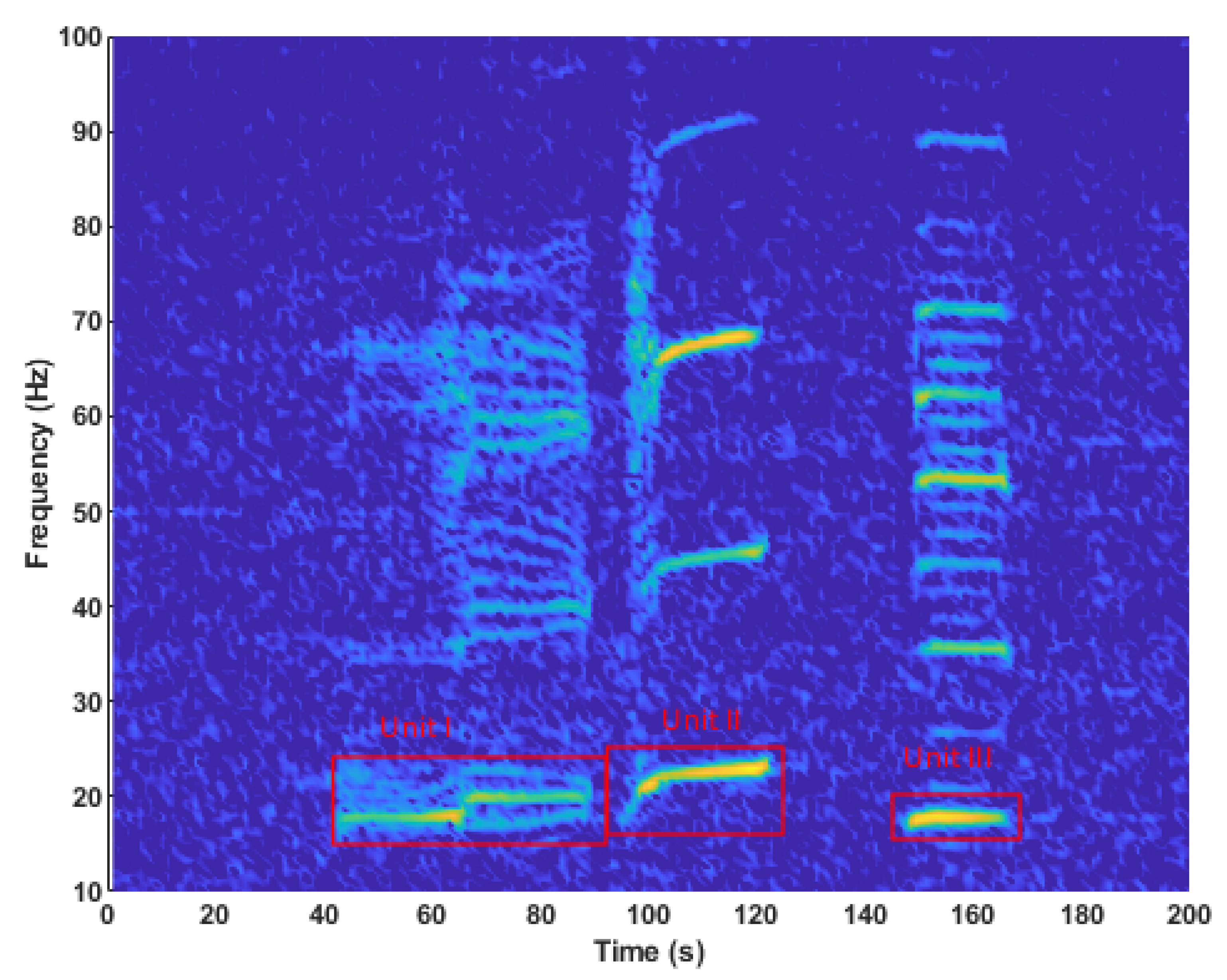
• (P2) Unit II, 20 s pause, then Unit III; and
• (P3) Unit I, 10 s pause, Unit II, 20 s pause, then Unit III [36,37,45].

Song templates were superimposed on the dive profile individually by selecting the start time of the song. The typical inter-song intervals (ISI) were not used as there is substantial variability between individuals [36,37]. A cross-correlation analysis in the time domain was conducted to verify the assignment of song templates to the dive profile.

The average patterns for fluking and pitch from the 58 dive profiles hypothesised to be the P3 song were the template signals for automated detection of P2 and P3 songs in the dive profile. The P2 template was from second 55 to the end of the P3 template. The P3 song is the same as P2, except it has an additional preceding unit. The MATLAB function xcorr with coeff normalisation compared the fluking and pitch templates to the corresponding time series for all proposed singing dives. The output correlation values from fluking and pitch templates were squared and multiplied together for a combined correlation value, so that there had to be a strong correlation in both time series for the signal to be classified as a song. Correlation values exceeding a threshold of 0.0005 were identified as the start times of the P2 and P3 songs. This threshold was determined by trialing a range of values to find the optimum true positive success rate with minimal false positive detections. Songs that were overlapping with surfacings were removed. If songs overlapped other songs, only the song with the greatest correlation value was retained. The manually identified songs were compared to songs detected automatically to identify inconsistencies, which were screened to rectify manual errors and confirm false positive results from the cross-correlation analysis. Only the songs that were common to both manual and automatic detection were used for further analyses.

2.6. Context of Sound Production

To determine the context of sound production over the duration of tag attachment, a simple multiple correlation analysis was conducted in the statistiXL software package (V2.0). Song Unit II was used as it had a characteristic descent that may be influenced by the ambient water temperature or the animal’s body condition. Unit II is also the most common and intense song unit that is commonly used in PAM research [1]. All Unit IIs from P2 and P3 songs that were common to manual and automatic identification methods were used. For each Unit II, the whale’s starting depth, final depth, depth change, median pitch, and external temperature (recorded by the tag) were determined and compared with each other and time.

2.7. Dive Type Classification Schema

An automated dive type classification schema was designed to assign each dive to a type (Figure 4). Six dive characteristics were used: maximum dive depth, median-to-maximum-depth ratio, dive duration, kicking rate, mean kick amplitude, and rate of heading change. The dive types were identified by manually comparing different dive profiles and assigning them to known behaviours. Thresholds were set by iterative improvements through a manual screening process of the dives grouped to types. The classification schema was verified for accuracy by conducting a Canonical Analysis of Principal Coordinates (CAP) and a leave-one-out cross validation on the dive type assignments and the six characteristics for each dive [46,47].

2.8. Behavioural Analysis

The behavioural context of song production was qualitatively analysed on three levels: individual dives, 3 h increments, and binary modes. The dive types used in the behavioural analysis were from the classification schema and not the reclassified groups from the CAP cross validation. Each 3 h increment was classified as a behavioural state based on the proportions of dive types, the distance travelled, amount of milling, location, and surrounding dives. The binary modes of foraging and migration were identified based on the behavioural states, the presence of feeding lunges, and the degree of milling.

Increments of 3 h were chosen to maximise the distinctiveness between behavioural states, enable delineation of twilight segments, and minimise the error in the milling proxy generated from low sample-rate location data (one position every 24 min on average). For each increment, the cumulative duration of each dive type was calculated and presented as a proportion of total time, including surface time. Surface time was calculated as the difference between the total increment duration and the sum of all dive type durations.

The distance travelled in each increment was calculated from the Fastloc GPS locations, including the total track length and the direct distance between the increment start and end location. A large difference between these values indicated that the whale was milling, while a small difference between total track length and direct distance indicated that the whale was travelling in a singular direction.

3. Results

3.1. Song Identified in the Dive Profile

There was substantial variability in the duration of and intervals between acoustically recorded EIOPB whale song units (Figure 5). In some songs, the Unit II started (minimum start was 58.2 s from time base) before Unit I from other songs had finished (maximum finish was 68.4 s from time base). Meanwhile, the Unit III in some songs finished (maximum 126.8 s) later than Unit III from other songs had started (minimum 122.7 s). As a result of the overlapping units when aligning instances of the P3 song from multiple animals, the average sound frequency track was heavily influenced by variation in song unit start and end times.

The EIOPB whale song structure corresponded to the proposed singing pattern in the dive profile. All proposed start and end times of the units identified from the dive profile fell within the temporal variability of the song structure and were closely aligned to the median values (Figure 5). The pattern was particularly consistent for pitch and fluking, which had low error margins over the duration of the window, especially during the gaps between kicking bouts.

3.2. Verification of Song Identification

The cross-correlation analysis identified P3 songs with a 97.6% true positive rate, finding 90.1% of the manually identified P3s (

Table 1. Results from the cross-correlation analysis comparing manually identified with automatically detected songs. Values are counts of songs. The percentage for manual songs is the proportion of songs manually identified that were automatically detected. Other percentages are the proportion of all cross-correlation (XC) signals. The wrong song column is the number of songs identified as the wrong song type.

Song	Manual Songs	XC Signals	XC Songs	Wrong Song	False Positives
P2	797 (91.3%)	907	728 (80.2%)	134 (14.8%)	45 (6.2%)
P3	1528 (90.1%)	1410	1376 (97.6%)	20 (1.4%)	15 (1.1%)

). Meanwhile the analysis identified P2 songs at an 80.2% true positive rate, finding 91.3% of the manually identified P2s. The cross-correlation analysis detected 8.8% of the manually identified P3s as P2s; in most of these samples the Unit I in the dive profile was shorter than in the P3 template. Visual inspection of all songs common to identification methods revealed that the signals identified as song were consistent with the fluking and pitch templates (Figure S1).

3.3. Context of Sound Production

From the 2325 songs common to both automatic and manual detection, a total of 6224 individual song units were identified in the dive profile including 1376 Unit Is, 2104 Unit IIs, and 2104 Unit IIIs. All song units were produced between 10 and 25 m depth. There were significant correlations between starting depth, final depth, depth change, pitch, and temperature during song Unit II production over the 7.6 days of tag attachment (Figure 6). The exception was between starting depth and median pitch, which were not significantly correlated.

As the whale migrated north, the water temperature measured by the tag during sound production, plus the whale’s sound production starting and finishing depths, all increased. The depth changes during sound production marginally increased with time and loosely correlated with the whale’s pitch. Meanwhile the whale’s pitch increased substantially with time, and to a lesser degree with increasing temperature. Starting depth had a stronger relationship with finishing depth than depth change.

3.4. Dive Type Classification Schema

The CAP cross-validation analysis classified 1197 of 1559 dives to the original groups (76.8%), which is significantly better than the 11.1% that would be correctly classified by random chance (Figure 7). All dive types had correct classification rates greater than 50% (Table S1). Shallow searching and intra-surfacing dive types had the lowest correctly classified rates, both having misclassification with each other, fast travel, and porpoising. Other sources of error were deep searching dives being misclassified as exploratory, fast travel as intra-surfacing, and resting as slow travel.

3.5. Behavioural Analysis

The low sample-rate of the Fastloc GPS locations was a limiting factor for the distance travelled measurement (Figure 8). The increments on 12 am 4 May and 9 am 5 May had just two locations making the milling proxy for these inaccurate. Five increments had between 3 and 5 locations and the remaining 54 increments had 6 locations or more. This was acceptable as most increments had sufficient locations to calculate the milling proxy, and if the increment duration were to be increased, the twilight-related singing behaviour would no longer be identifiable. A map of the spatial distribution of dive types can be found in the Supplementary Materials (Figure S2).

3.5.1. Behavioural States

The five behavioural states across time are shown in Figure 8 where they are distinguished as feeding, travelling, milling, resting, and social. Travelling was identified by a low degree of milling and a high proportion of slow travel dives, which included exploratory and resting dives (Figure 8). The whale travelled primarily between dawn and dusk. On average, the whale produced a similar number of P2 and P3 song types while travelling, except during the night when P3 songs were 2.7 times more prevalent (

Table 2. The number of Unit II vocalisations, P2, and P3 song types produced per h, and the proportion of time the whale spent in singing dives are presented for three behavioural categories: the migratory behavioural mode, and the milling and travelling states. The other behavioural states and modes were not included as the whale did not sing during these periods and there was a limited sample size of these behaviours. The behaviours were analysed in time-of-day groups and cumulatively. Duration is the time spent in that behavioural category over the whole tag attachment. Time in singing dives is total dive time of all singing dives in that category divided by total duration of the category.

	Total Duration (h)	Unit II h−1	P2 Songs h−1	P3 Songs h−1	Time in Singing Dives (%)
Migrating	171	13.6	4.6	9.0	73.8%
Day	63	15.2	6.6	8.5	76.8%
Night	66	10.6	1.9	8.6	64.9%
Twilight	42	15.9	5.8	10.2	83.3%
Milling	57	8.8	0.8	8.0	56.9%
Day	9	7.1	0.0	7.0	48.1%
Night	36	8.3	0.8	7.6	53.6%
Twilight	12	11.6	1.5	10.2	73.4%
Travelling	111	16.1	6.7	9.4	82.4%
Day	54	16.6	7.7	8.8	81.6%
Night	27	13.4	3.6	9.7	78.7%
Twilight	30	17.6	7.5	10.2	87.3%

). However, fine-scale variability was observed: on 5 May, the whale produced more P2 songs at dawn and dusk but more P3 songs and exploratory dives during the day. On 1 and 7 May, the opposite trend was observed, when P2 song production peaked during the day rather than at twilight and less time was spent in exploratory dives during the day. The whale was singing in most slow travelling and exploratory dives (

Table 3. The characteristics of each dive type, divided into those with feeding lunges (F) and when the whale was singing (S). Mean values have +/− standard deviation. N is the number of dives assigned to the type.

Dive Type	N	Total Duration (h)	Surface Interval (s)	Blows	Dive Duration (min)	Mean Bottom Depth (m)
Deep searching	21	3.36	56.9 ± 36.5	4.4 ± 2.5	9.5 ± 3.3	189 ± 163
Deep searching (F)	8	1.79	150.4 ± 40.1	11.3 ± 2.6	13.4 ± 2.7	354 ± 97
Exploratory	14	2.87	93.6 ± 52.8	5.6 ± 2.4	12.3 ± 6.8	30 ± 18
Exploratory (S)	21	4.51	68.9 ± 44.0	4.3 ± 2.0	12.8 ± 4.6	44 ± 56
Fast travel	109	8.23	71.8 ± 67.8	4.5 ± 3.8	4.5 ± 4.0	21 ± 13
Fast travel (S)	5	0.68	46.2 ± 13.8	3.2 ± 0.9	8.1 ± 1.4	21 ± 3
Intra surfacing	231	1.03	16.4 ± 31.5	1.8 ± 1.7	0.2 ± 0.1	4 ± 2
Porpoising	205	1.71	2.1 ± 4.8	1.0 ± 0.2	0.5 ± 0.4	12 ± 6
Racing	10	0.53	1.8 ± 0.6	1.0 ± 0.0	3.1 ± 1.3	53 ± 21
Resting	33	3.02	70.1 ± 31.3	4.3 ± 1.8	5.4 ± 3.4	7 ± 6
Resting (S)	8	2.25	203.0 ± 347.1	8.0 ± 9.9	16.8 ± 4.1	15 ± 2
Shallow searching	85	4.37	27.7 ± 30.3	2.3 ± 1.5	3.0 ± 3.0	18 ± 9
Shallow searching (S)	8	1.19	43.4 ± 22.5	3.0 ± 1.2	8.9 ± 4.4	20 ± 4
Slow travel	130	8.75	79.6 ± 81.5	4.7 ± 4.3	4.0 ± 3.6	12 ± 8
Slow travel (S)	671	117.98	57.5 ± 53.1	3.5 ± 2.1	10.5 ± 4	18 ± 2

). The milling behavioural state was identified by a high degree of milling and a higher proportion of searching, exploratory, and fast travel dives than during travelling (Figure 8). The whale milled more during the night, except during the day on 2 May, when it conducted a lot of searching dives. During milling, the whale almost exclusively produced P3 song types and spent a lower proportion of time singing than while in a travelling state (Table 2).

3.5.2. Behavioural Modes

From the behavioural states, two behavioural modes were identified: foraging and migration (Figure 8). The foraging behavioural mode was not well defined as the duration of the feeding behavioural state was limited. Further, all observed singing was during the migratory mode, so a relationship between singing and foraging was not established. The whale spent more time singing during the day than at night while migrating, and most during the twilight periods (Table 2).

3.5.3. Surface Activity

The proportion of time spent at the surface had a weak relationship with the 3 h behavioural states (Figure 8), but there was a clear relationship between surface time and dive type (Table 3). Peaks in proportion of time spent at the surface occurred after the foraging period, and after periods of milling behaviour where there was a relatively high proportion of searching dives. The least time was spent at the surface between porpoising and racing dives when the whale rarely conducted more than a single blow per surfacing. The most blows per surfacing were between deep searching dives when the whale was feeding. When feeding, the whale dived deeper and longer than when on non-feeding deep-searching dives and spent longer at the surface between dives. The whale spent the most time at the surface between resting dives when the whale was singing. During non-singing resting dives, the whale was at an average depth of 7 ± 6 m and made almost zero kicks during dives.

4. Discussion

By linking patterns in dive profile characteristics with EIOPB whale song structure, the context of EIOPB whale sound production was determined for a single animal over 7.6 days. The depth of sound production was positively correlated to the duration of migration and water temperature, indicating that the optimal singing depth may vary with time and environmental conditions. A novel automated classification schema was developed to describe the whale’s diving behaviour, which was used as the basis for classification into 3 h states and binary modes. The three levels of behavioural classification had different relationships with singing. The 3 h states during migration displayed relationships that will facilitate more accurate PAM abundance estimates.

4.1. Limitations of Study

Our description of the behavioural context of song produced by EIOPB whales was limited by a sample size of one animal, a tag attachment duration of 7.6 days, and a single behavioural mode (migration) for most of the tag attachment. As a result, we cannot infer the behavioural context of singing for the entire EIOPB whale population across their broad geographical range and the various behaviours they may employ during migration, social events, and foraging. Further, as there were no nearby simultaneous acoustic recordings during the singing dives, there remains an element of uncertainty in the identification of song using only the dive profile. Identifying repetitive song sequences from dive profiles is also limited to investigation of behaviours related to song, as we have not yet identified if dive profiles can be linked to non-song vocalisations [36,48]. As the pattern in depth was the most variable during sound production, biotelemetry with only pressure sensor data is unreliable for song identification. Through automated song detection, we have shown that recording the whale’s attitude is required to identify song from the dive profile, which can only currently be achieved with retrievable tags. High sample-rate accelerometer and acoustic tags that can empirically record song attributable to the tagged whale should be used for the research of singing whales using biotelemetry [49,50,51].

4.2. Physical Context of Song

There are unexplained Mysticeti intra- and inter-annual song frequency shifts that have been hypothesised (but not proven) to be the result of cultural drivers, seasonal phenomena such as sea-ice noise, increased ambient sea noise, variation in the density of singing animals, whale body condition, a change in average size of animals recovering from whaling, and climate change [2,45,52,53,54,55,56,57]. Varied singing depths by great whales have also been suggested to contribute to these sound frequency trends [45]. We have demonstrated that as an EIOPB whale migrated north from a feeding location into warmer waters, it adjusted its singing depth by starting vocalisations shallower.

The depth-dependent frequency-shift hypothesis has been previously discounted because there is no explanation for whales collectively changing singing depth [2,56], and singing depths appear to vary in short time periods for individuals [5]. On closer inspection, sounds of the same unit type within a single singing bout were produced at consistent depths, as has been demonstrated here and by Lewis et al. (2018). While we observed variation in depth (~5 m range) within a given day of Unit IIs produced, there was a significant positive correlation between singing depth and time. While the driver of this depth preference is not yet clear, it is the first indication that blue whales sing at varying depths.

Whales might exploit a “sweet depth” for sound production. In the austral winter when pygmy blue whales migrate along the Western Australian coast, the temperature profile of the water leads to a variable acoustic duct within the top ~50 m of water [58]. In this surface duct, sound may propagate at little loss over long ranges, a phenomenon these whales might exploit for both sound production and reception (as suggested earlier by [59]).

As the whale was primarily travelling while singing, the singing depth could also be driven by the desire to be neutrally buoyant and to minimise surface drag [60]. The singing depth and descent during sound production were not closely correlated to the whale’s pitch, so the strong correlation between pitch and time may be to account for decreasing buoyancy. After feeding in the Perth Canyon, the whale migrated north without feeding again, likely resulting in a steadily decreasing body condition. If body condition decreased, so too would buoyancy, which would be compounded by the increasing water temperature [61,62]. Variable body condition and water temperature may provide a biological basis to explain why whales sing at different depths.

4.3. Classification of Diving Behaviour

While not without limitations, our automated dive classification schema removes manual error or bias, allows rapid classification for large datasets, and provides a schema that can be consistent across multiple datasets. Application of the classification schema with other datasets will require altering accelerometer derived thresholds to account for different locations of tag attachment, cetacean species, and tag types. The CAP analysis confirmed that dive types were distinctive from one another. Some misclassifications between the CAP and automated classification were expected, as the CAP uses principal components of all characteristics to separate types [46,47], while the automated classification schema often used just one or two characteristics. Fonseca et al. (2022) employed principal component analysis with hierarchical clustering to automate dive classification and concluded that the method could over-generalise the complex spectrum of behaviour, especially for under-represented behaviours. Alternatively, the discrete classification schema used in this study empowered our identification of niche behaviours such as porpoising, highlighting that these two classification methods support each other well.

The niche behaviour identified in this study as porpoising may represent a social interaction but was previously identified as surface feeding [31]. Owen et al. identified this period as surface feeding as they did not use blanking periods in their criterion and did not have the fluking time series to support their identification of feeding lunges. When the EIOPB whale conducted a feeding lunge, we expected to see a blanking period, defined as when a whale stops swimming to filter krill from the engulfed seawater by contracting the ventral pleats [40,43,63]. Rather, throughout the surface-active period, the whale maintained a high rate of incessant fluking with large kick amplitudes, and continuous large amplitude responses in the accelerometer record. The porpoising and racing period was thought to be social behaviour as EIOPB whales have been observed conducting similar surface activity while interacting with conspecifics in mating displays [9,64,65,66]. Alternatively, it could represent evasive behaviour from killer whales (Orcinus orca), which have been observed near where this behaviour occurred [67,68]. The defined dive types such as porpoising formed the base units for behavioural classification of 3 h states and binary modes, providing insights into the behavioural context of song production.

4.4. Singing Behavioural Context

For the approximately 7 days of migration, the EIOPB whale spent more time on singing dives during the day (76.8%) than at night (64.9%), but song production was greatest during the twilight periods (83.3%). Oestreich et al. [13] also linked migration to higher singing rates during the day for eastern North Pacific blue whales, while foraging was associated with night-time singing. The whale tagged here did not spend long enough foraging for us to make the same association. However, EIOPB whales have been found to sing more at night than day in the foraging grounds of Perth Canyon based on PAM [69]. During the migration of the tagged whale, the finer-scaled behavioural states of travelling and milling were associated with different song production regimes.

The whale travelled more during the day than night, producing a similar number of P2 and P3 song types. This may be to increase the rate of Unit IIs produced, which is their most intense vocalisation and so can be heard from farthest away [36]. This may aid navigation for other whales [11], or be to broadcast its reproductive fitness according to the Adam et al. (2013) 4Ls theory. The 4Ls theory states that a whale will advertise its fitness through intense (loud) low-frequency and long units that can be heard from a long range, and that it will sing persistently (loquacious) to compete with other singers [8].

The whale tagged here almost exclusively produced the P3 song type during milling. Milling during migration may be related to food searching, which is expected as EIOPB whales feed year-round [27,28]. Alternatively, the whale might have been searching for conspecifics or a mate. The whale milled more during the night than day, which may be a better time to find food because their neritic and mesophotic prey converge to the same depth stratum. As night falls, mesophotic krill rise to the surface, where the neritic krill exist [35,70], so the probability of finding prey is higher. The different song types produced while milling and travelling suggest that EIOPB whales use subtle vocal cues to communicate their behaviour.

Defining a relationship between behaviour and sound production is crucial for making blue whale abundance estimates with PAM, but describing only the behavioural context of singing as a binary mode without considering the behavioural state could overlook drivers of sound production variability. Oestreich et al. [13] defined an inversely proportional ratio of singing rate during night versus day between migratory and foraging modes. However, there is variability in sound production rates during the migration reported by Oestreich et al., which may be accounted for by behavioural states and delineation of song types as we have indicated, as well as non-song versus song vocalisations [5]. PAM of singing rates may have power to detect the average population behavioural mode using the defined diel variation in song production identified by Oestreich et al., but achieving abundance estimates requires finer contextual resolution of sound production variability. Meanwhile, using classified dives (i.e., a period equal to the mean dive time [5]) as the behavioural unit will identify the dive type related to sound production, but not necessarily the broader context of singing. As dive durations can be up to 30 min, the 3 h period used here is a reasonable duration to describe the behavioural context of singing, which would be beneficial for making PAM derived abundance estimates.

5. Conclusions

We developed a novel method to identify singing from patterns in this pygmy blue whale’s dive profile, revealing preliminary evidence that sound production depth could be linked to ocean temperature and whale body condition, which may influence the sound frequency produced. Future work should investigate the relationship between water temperature, song frequency, and body condition of great whales to determine if the intra- and inter-annual song frequency trends can be explained by ocean warming and life history strategies. While we also have preliminarily described the behavioural context of song production, further research into the sound production context, the proportion and demographic of the population that sings, and the percentage of time whales spend singing is required to make accurate population abundance measurements with PAM.

The automated dive type classification schema developed here provides a precedent for a standardised behavioural analysis method, which could be improved with tag datasets from multiple animals to account for variability in tag attachment location. Including attitude and fluking rates in behavioural classification with the shallowest reasonable dive delineation threshold (1.5 m) has enabled the detection of shallow resting dives that are well within the lethal strike depth of commercial ships. These resting dives need to be investigated further to manage ship strike risk.

References

1. McCauley, R.D.; Gavrilov, A.N.; Jolliffe, C.D.; Ward, R.; Gill, P.C. Pygmy Blue and Antarctic Blue Whale Presence, Distribution and Population Parameters in Southern Australia Based on Passive Acoustics. Deep Sea Res. Part II Top. Stud. Oceanogr. 2018, 157–158, 154–168. [Google Scholar] [CrossRef]
2. Rice, A.; Širović, A.; Hildebrand, J.A.; Wood, M.; Carbaugh-Rutland, A.; Baumann-Pickering, S. Update on Frequency Decline of Northeast Pacific Blue Whale (Balaenoptera musculus) Calls. PLoS ONE 2022, 17, e0266469. [Google Scholar] [CrossRef] [PubMed]
3. Dziak, R.P.; Haxel, J.H.; Lau, T.-K.; Heimlich, S.; Caplan-Auerbach, J.; Mellinger, D.K.; Matsumoto, H.; Mate, B. A Pulsed-Air Model of Blue Whale B Call Vocalizations. Sci. Rep. 2017, 7, 9122. [Google Scholar] [CrossRef] [PubMed]
4. Oleson, E.M.; Calambokidis, J.; Burgess, W.C.; McDonald, M.A.; LeDuc, C.A.; Hildebrand, J.A. Behavioral Context of Call Production by Eastern North Pacific Blue Whales. Mar. Ecol. Prog. Ser. 2007, 330, 269–284. [Google Scholar] [CrossRef]
5. Lewis, L.A.; Calambokidis, J.; Stimpert, A.K.; Fahlbusch, J.; Friedlaender, A.S.; McKenna, M.F.; Mesnick, S.L.; Oleson, E.M.; Southall, B.L.; Szesciorka, A.R.; et al. Context-Dependent Variability in Blue Whale Acoustic Behaviour. R. Soc. Open Sci. 2018, 5, 180241. [Google Scholar] [CrossRef] [PubMed]
6. McDonald, M.A.; Calambokidis, J.; Teranishi, A.M.; Hildebrand, J.A. The Acoustic Calls of Blue Whales off California with Gender Data. J. Acoust. Soc. Am. 2001, 109, 1728–1735. [Google Scholar] [CrossRef] [PubMed]
7. Cazau, D.; Adam, O.; Aubin, T.; Laitman, J.T.; Reidenberg, J.S. A Study of Vocal Nonlinearities in Humpback Whale Songs: From Production Mechanisms to Acoustic Analysis. Sci. Rep. 2016, 6, 31660. [Google Scholar] [CrossRef]
8. Adam, O.; Cazau, D.; Gandilhon, N.; Fabre, B.; Laitman, J.T.; Reidenberg, J.S. New Acoustic Model for Humpback Whale Sound Production. Appl. Acoust. 2013, 74, 1182–1190. [Google Scholar] [CrossRef]
9. Schall, E.; Di Iorio, L.; Berchok, C.; Filún, D.; Bedriñana-Romano, L.; Buchan, S.J.; Van Opzeeland, I.; Sears, R.; Hucke-Gaete, R. Visual and Passive Acoustic Observations of Blue Whale Trios from Two Distinct Populations. Mar. Mamm. Sci. 2020, 36, 365–374. [Google Scholar] [CrossRef]
10. Tyack, P.L. Studying How Cetaceans Use Sound to Explore Their Environment. In Communication; Owings, D.H., Beecher, M.D., Thompson, N.S., Eds.; Springer: Boston, MA, USA, 1997; pp. 251–297. ISBN 9781489917454. [Google Scholar]
11. Payne, R.; Webb, D. Orientation by Means of Long Range Acoustic Signaling in Baleen Whales. Ann. N. Y. Acad. Sci. 1971, 188, 110–141. [Google Scholar] [CrossRef]
12. Clark, C.W.; Ellison, W.T. Potential Use of Low-Frequency Sounds by Baleen Whales for Probing the Environment: Evidence from Models and Empirical Measurements. In Echolocation in Bats and Dolphins; The University of Chicago Press: Chicago, IL, USA, 2004. [Google Scholar]
13. Oestreich, W.K.; Fahlbusch, J.A.; Cade, D.E.; Calambokidis, J.; Margolina, T.; Joseph, J.; Friedlaender, A.S.; McKenna, M.F.; Stimpert, A.K.; Southall, B.L.; et al. Animal-Borne Metrics Enable Acoustic Detection of Blue Whale Migration. Curr. Biol. 2020, 30, 4773–4779.e3. [Google Scholar] [CrossRef]
14. Aroyan, J.L.; McDonald, M.A.; Webb, S.C.; Hildebrand, J.A.; Clark, D.; Laitman, J.T.; Reidenberg, J.S. Acoustic Models of Sound Production and Propagation. In Hearing by Whales and Dolphins; Au, W.W.L., Fay, R.R., Popper, A.N., Eds.; Springer: New York, NY, USA, 2000; pp. 409–469. ISBN 9781461211501. [Google Scholar]
15. Stimpert, A.K.; DeRuiter, S.L.; Falcone, E.A.; Joseph, J.; Douglas, A.B.; Moretti, D.J.; Friedlaender, A.S.; Calambokidis, J.; Gailey, G.; Tyack, P.L.; et al. Sound Production and Associated Behavior of Tagged Fin Whales (Balaenoptera Physalus) in the Southern California Bight. Anim. Biotelemetry 2015, 3, 23. [Google Scholar] [CrossRef]
16. Jones, A.D.; McCauley, R.D.; Cato, D.H. Observations and Explanation of Low Frequency Clicks in Blue Whale Calls. In Proceedings of the Annual Conference of the Australian Acoustical Society, Adelaide, Australia, 12–15 November 2002; pp. 45–50. [Google Scholar]
17. Brekhovskikh, L.M.; Lysanov, Y.P.; Lysanov, J.P. Fundamentals of Ocean Acoustics; Springer Science & Business Media: Berlin/Heidelberg, Germany, 2003; ISBN 9780387954677. [Google Scholar]
18. Hooker, S.K.; Fahlman, A.; Moore, M.J.; de Soto, N.A.; de Quirós, Y.B.; Brubakk, A.O.; Costa, D.P.; Costidis, A.M.; Dennison, S.; Falke, K.J.; et al. Deadly Diving? Physiological and Behavioural Management of Decompression Stress in Diving Mammals. Proc. Biol. Sci. 2012, 279, 1041–1050. [Google Scholar] [CrossRef]
19. Bostrom, B.L.; Fahlman, A.; Jones, D.R. Tracheal Compression Delays Alveolar Collapse during Deep Diving in Marine Mammals. Respir. Physiol. Neurobiol. 2008, 161, 298–305. [Google Scholar] [CrossRef]
20. Moore, M.J.; Hammar, T.; Arruda, J.; Cramer, S.; Dennison, S.; Montie, E.; Fahlman, A. Hyperbaric Computed Tomographic Measurement of Lung Compression in Seals and Dolphins. J. Exp. Biol. 2011, 214, 2390–2397. [Google Scholar] [CrossRef]
21. Bouffaut, L.; Landrø, M.; Potter, J.R. Source Level and Vocalizing Depth Estimation of Two Blue Whale Subspecies in the Western Indian Ocean from Single Sensor Observations. J. Acoust. Soc. Am. 2021, 149, 4422–4436. [Google Scholar] [CrossRef]
22. Branch, T.A.; Stafford, K.M.; Palacios, D.M.; Allison, C.; Bannister, J.L.; Burton, C.L.K.; Cabrera, E.; Carlson, C.A.; Galletti Vernazzani, B.; Gill, P.C.; et al. Past and Present Distribution, Densities and Movements of Blue Whales Balaenoptera Musculus in the Southern Hemisphere and Northern Indian Ocean. Mamm. Rev. 2007, 37, 116–175. [Google Scholar] [CrossRef]
23. Thums, M.; Ferreira, L.; Jenner, C.; Jenner, M.; Harris, D.; Davenport, A.; Andrews-Goff, V.; Double, M.; Möller, L.; Attard, C.R.M.; et al. Pygmy Blue Whale Movement, Distribution and Important Areas in the Eastern Indian Ocean. Glob. Ecol. Conserv. 2022, 35, e02054. [Google Scholar] [CrossRef]
24. McCauley, R.D.; Jenner, C. Migratory Patterns and Estimated Population Size of Pygmy Blue Whales (Balaenoptera Musculus Brevicauda) Traversing the Western Australian Coast Based on Passive Acoustics. In Paper SC/62/SH26 Presented to the IWC Scientific Committee, Agadir, Morocco, 21–25 June 2010; International Whaling Commission: Cambridge, UK.
25. Samaran, F.; Stafford, K.M.; Branch, T.A.; Gedamke, J.; Royer, J.-Y.; Dziak, R.P.; Guinet, C. Seasonal and Geographic Variation of Southern Blue Whale Subspecies in the Indian Ocean. PLoS ONE 2013, 8, e71561. [Google Scholar] [CrossRef]
26. Leroy, E.C.; Samaran, F.; Stafford, K.M.; Bonnel, J.; Royer, J.Y. Broad-Scale Study of the Seasonal and Geographic Occurrence of Blue and Fin Whales in the Southern Indian Ocean. Endanger. Species Res. 2018, 37, 289–300. [Google Scholar] [CrossRef] [Green Version]
27. Möller, L.M.; Attard, C.R.M.; Bilgmann, K.; Andrews-Goff, V.; Jonsen, I.; Paton, D.; Double, M.C. Movements and Behaviour of Blue Whales Satellite Tagged in an Australian Upwelling System. Sci. Rep. 2020, 10, 21165. [Google Scholar] [CrossRef]
28. Double, M.C.; Andrews-Goff, V.; Jenner, K.C.S.; Jenner, M.-N.; Laverick, S.M.; Branch, T.A.; Gales, N.J. Migratory Movements of Pygmy Blue Whales (Balaenoptera musculus Brevicauda) between Australia and Indonesia as Revealed by Satellite Telemetry. PLoS ONE 2014, 9, e93578. [Google Scholar] [CrossRef]
29. Andrews-Goff, V.; Bestley, S.; Gales, N.J.; Laverick, S.M.; Paton, D.; Polanowski, A.M.; Schmitt, N.T.; Double, M.C. Humpback Whale Migrations to Antarctic Summer Foraging Grounds through the Southwest Pacific Ocean. Sci. Rep. 2018, 8, 12333. [Google Scholar] [CrossRef]
30. Kahn, B. Blue Whales of the Savu Sea, Indonesia. In Proceedings of the 17th Biennial Conference on the Biology of Marine Mammals, Cape Town, South Africa, 28 November–3 December 2007; p. 89. [Google Scholar]
31. Owen, K.; Jenner, C.S.; Jenner, M.-N.M.; Andrews, R.D. A Week in the Life of a Pygmy Blue Whale: Migratory Dive Depth Overlaps with Large Vessel Drafts. Anim. Biotelemetry 2016, 4, 17. [Google Scholar] [CrossRef]
32. Conservation Management Plan for the Blue Whale: A Recovery Plan under the Environment Protection and Biodiversity Conservation Act 1999, Commonwealth of Australia 2015. Available online: https://www.dcceew.gov.au/sites/default/files/documents/blue-whale-conservation-management-plan.pdf (accessed on 15 October 2021).
33. Branch, T.A.; Allison, C.; Mikhalev, Y.A.; Tormosov, D.; Brownell, R.L. Historical Catch Series for Antarctic and Pygmy Blue Whales. In Paper SC/60/SH9 Presented to the IWC Scientific Committee, Santiago, Chile, 23–27 June 2008; International Whaling Commission: Cambridge, UK.
34. Jenner, C.; Jenner, M.; Burton, C.; Sturrock, V.; Kent, C.S.; Morrice, M.; Attard, C.; Möller, L.; Double, M.C. Mark Recapture Analysis of Pygmy Blue Whales from the Perth Canyon, Western Australia 2000–2005. In Paper SC/60/SH16 Presented to the IWC Scientific Committee, Santiago, Chile, 23–27 June 2008; International Whaling Commission: Cambridge, UK.
35. Rennie, S.; Hanson, C.E.; McCauley, R.D.; Pattiaratchi, C.; Burton, C.; Bannister, J.; Jenner, C.; Jenner, M.-N. Physical Properties and Processes in the Perth Canyon, Western Australia: Links to Water Column Production and Seasonal Pygmy Blue Whale Abundance. J. Mar. Syst. 2009, 77, 21–44. [Google Scholar] [CrossRef]
36. Jolliffe, C.D.; McCauley, R.D.; Gavrilov, A.N.; Jenner, K.C.S.; Jenner, M.-N.M.; Duncan, A.J. Song Variation of the South Eastern Indian Ocean Pygmy Blue Whale Population in the Perth Canyon, Western Australia. PLoS ONE 2019, 14, e0208619. [Google Scholar] [CrossRef]
37. Jolliffe, C.D.; McCauley, R.D.; Gavrilov, A.N.; Jenner, C.; Jenner, M.N. Comparing the Acoustic Behaviour of the Eastern Indian Ocean Pygmy Blue Whale on Two Australian Feeding Grounds. Acoust. Aust. 2021, 49, 331–344. [Google Scholar] [CrossRef]
38. Marques, T.A.; Thomas, L.; Martin, S.W.; Mellinger, D.K.; Ward, J.A.; Moretti, D.J.; Harris, D.; Tyack, P.L. Estimating Animal Population Density Using Passive Acoustics. Biol. Rev. Camb. Philos. Soc. 2013, 88, 287–309. [Google Scholar] [CrossRef] [PubMed]
39. Cade, D.E.; Gough, W.T.; Czapanskiy, M.F.; Fahlbusch, J.A.; Kahane-Rapport, S.R.; Linsky, J.M.J.; Nichols, R.C.; Oestreich, W.K.; Wisniewska, D.M.; Friedlaender, A.S.; et al. Tools for Integrating Inertial Sensor Data with Video Bio-Loggers, Including Estimation of Animal Orientation, Motion, and Position. Anim. Biotelemetry 2021, 9, 34. [Google Scholar] [CrossRef]
40. Simon, M.; Johnson, M.; Madsen, P.T. Keeping Momentum with a Mouthful of Water: Behavior and Kinematics of Humpback Whale Lunge Feeding. J. Exp. Biol. 2012, 215, 3786–3798. [Google Scholar] [CrossRef] [PubMed] [Green Version]
41. Goldbogen, J.A.; Calambokidis, J.; Shadwick, R.E.; Oleson, E.M.; McDonald, M.A.; Hildebrand, J.A. Kinematics of Foraging Dives and Lunge-Feeding in Fin Whales. J. Exp. Biol. 2006, 209, 1231–1244. [Google Scholar] [CrossRef] [PubMed]
42. Owen, K.; Dunlop, R.A.; Monty, J.P.; Chung, D.; Noad, M.J.; Donnelly, D.; Goldizen, A.W.; Mackenzie, T. Detecting Surface-Feeding Behavior by Rorqual Whales in Accelerometer Data. Mar. Mamm. Sci. 2016, 32, 327–348. [Google Scholar] [CrossRef]
43. Sweeney, D.A.; DeRuiter, S.L.; McNamara-Oh, Y.J.; Marques, T.A.; Arranz, P.; Calambokidis, J. Automated Peak Detection Method for Behavioral Event Identification: Detecting Balaenoptera musculus and Grampus griseus Feeding Attempts. Anim. Biotelemetry 2019, 7, 7. [Google Scholar] [CrossRef]
44. Erbe, C.; Verma, A.; McCauley, R.; Gavrilov, A.; Parnum, I. The Marine Soundscape of the Perth Canyon. Prog. Oceanogr. 2015, 137, 38–51. [Google Scholar] [CrossRef]
45. Gavrilov, A.N.; McCauley, R.D.; Salgado-Kent, C.; Tripovich, J.; Burton, C. Vocal Characteristics of Pygmy Blue Whales and Their Change over Time. J. Acoust. Soc. Am. 2011, 130, 3651–3660. [Google Scholar] [CrossRef]
46. Anderson, M.J.; Willis, T.J. Canonical Analysis of Principal Coordinates: A Useful Method of Constrained Ordination for Ecology. Ecology 2003, 84, 511–525. [Google Scholar] [CrossRef]
47. Anderson, M.J.; Robinson, J. Generalized Discriminant Analysis Based on Distances. Aust. N. Z. J. Stat. 2003, 45, 301–318. [Google Scholar] [CrossRef]
48. Recalde-Salas, A.; Salgado Kent, C.P.; Parsons, M.J.G.; Marley, S.A.; McCauley, R.D. Non-Song Vocalizations of Pygmy Blue Whales in Geographe Bay, Western Australia. J. Acoust. Soc. Am. 2014, 135, EL213–EL218. [Google Scholar] [CrossRef]
49. Stimpert, A.K.; Lammers, M.O.; Pack, A.A.; Au, W.W.L. Variations in Received Levels on a Sound and Movement Tag on a Singing Humpback Whale: Implications for Caller Identification. J. Acoust. Soc. Am. 2020, 147, 3684. [Google Scholar] [CrossRef]
50. Goldbogen, J.A.; Stimpert, A.K.; DeRuiter, S.L.; Calambokidis, J.; Friedlaender, A.S.; Schorr, G.S.; Moretti, D.J.; Tyack, P.L.; Southall, B.L. Using Accelerometers to Determine the Calling Behavior of Tagged Baleen Whales. J. Exp. Biol. 2014, 217, 2449–2455. [Google Scholar] [CrossRef] [Green Version]
51. Saddler, M.R.; Bocconcelli, A.; Hickmott, L.S.; Chiang, G.; Landea-Briones, R.; Bahamonde, P.A.; Howes, G.; Segre, P.S.; Sayigh, L.S. Characterizing Chilean Blue Whale Vocalizations with DTAGs: A Test of Using Tag Accelerometers for Caller Identification. J. Exp. Biol. 2017, 220, 4119–4129. [Google Scholar] [CrossRef]
52. Miller, B.S.; Leaper, R.; Calderan, S.; Gedamke, J. Red Shift, Blue Shift: Investigating Doppler Shifts, Blubber Thickness, and Migration as Explanations of Seasonal Variation in the Tonality of Antarctic Blue Whale Song. PLoS ONE 2014, 9, e107740. [Google Scholar] [CrossRef]
53. Gavrilov, A.N.; McCauley, R.D.; Gedamke, J. Steady Inter and Intra-Annual Decrease in the Vocalization Frequency of Antarctic Blue Whales. J. Acoust. Soc. Am. 2012, 131, 4476–4480. [Google Scholar] [CrossRef]
54. Leroy, E.C.; Royer, J.-Y.; Bonnel, J.; Samaran, F. Long-Term and Seasonal Changes of Large Whale Call Frequency in the Southern Indian Ocean. J. Geophys. Res. C Oceans 2018, 123, 8568–8580. [Google Scholar] [CrossRef]
55. McDonald, M.A.; Hildebrand, J.A.; Mesnick, S. Worldwide Decline in Tonal Frequencies of Blue Whale Songs. Endanger. Species Res. 2009, 9, 13–21. [Google Scholar] [CrossRef]
56. Malige, F.; Patris, J.; Hauray, M.; Giraudet, P.; Glotin, H. Camille Noûs Mathematical Models of Long Term Evolution of Blue Whale Song Types’ Frequencies. J. Theor. Biol. 2022, 548, 111184. [Google Scholar] [CrossRef]
57. Malige, F.; Patris, J.; Buchan, S.J.; Stafford, K.M.; Shabangu, F.; Findlay, K.; Hucke-Gaete, R.; Neira, S.; Clark, C.W.; Glotin, H. Inter-Annual Decrease in Pulse Rate and Peak Frequency of Southeast Pacific Blue Whale Song Types. Sci. Rep. 2020, 10, 8121. [Google Scholar] [CrossRef]
58. Erbe, C.; Peel, D.; Smith, J.N.; Schoeman, R.P. Marine Acoustic Zones of Australia. J. Mar. Sci. Eng. 2021, 9, 340. [Google Scholar] [CrossRef]
59. Barham, E.G. Whales’ Respiratory Volume as a Possible Resonant Receiver for 20 Hz Signals. Nature 1973, 245, 220–221. [Google Scholar] [CrossRef]
60. Hertel, H. Structure-Form-Movement; Reinhold: New York, NY, USA, 1966; ISBN 9780442150570. [Google Scholar]
61. Thums, M.; Bradshaw, C.J.A.; Hindell, M.A. Tracking Changes in Relative Body Composition of Southern Elephant Seals Using Swim Speed Data. Mar. Ecol. Prog. Ser. 2008, 370, 249–261. [Google Scholar] [CrossRef] [Green Version]
62. Goldman, J.A. Effects of the Free Water Surface on Animals That Jump out of Water; Duke University: Ann Arbor, MI, USA, 2001. [Google Scholar]
63. Palacios, D.M.; Irvine, L.M.; Lagerquist, B.A.; Fahlbusch, J.A.; Calambokidis, J.; Tomkiewicz, S.M.; Mate, B.R. A Satellite-Linked Tag for the Long-Term Monitoring of Diving Behavior in Large Whales. Anim. Biotelemetry 2021, 10, 26. [Google Scholar] [CrossRef]
64. de Vos, A.; Brownell, R.L.; Tershy, B.; Croll, D. Anthropogenic Threats and Conservation Needs of Blue Whales, Balaenoptera Musculus Indica, around Sri Lanka. J. Mar. Biol. 2016, 2016, 8420846. [Google Scholar] [CrossRef]
65. Jenner, K.C.S. (Centre for Whale Research (WA) Inc., Fremantle, WA, Australia); Jenner, M.M. (Centre for Whale Research (WA) Inc., Fremantle, WA, Australia). Personal communication. 2022. [Google Scholar]
66. Gill, P. (Deakin University, Warrnambool, VIC, Australia). Personal communication, 2022.
67. Donnelly, D.M.; McInnes, J.D.; Jenner, K.C.S.; Jenner, M.-N.M.; Morrice, M. The First Records of Antarctic Type B and C Killer Whales (Orcinus orca) in Australian Coastal Waters. Aquat. Mamm. 2021, 47, 292–302. [Google Scholar] [CrossRef]
68. Totterdell, J.A.; Wellard, R.; Reeves, I.M.; Elsdon, B.; Markovic, P.; Yoshida, M.; Fairchild, A.; Sharp, G.; Pitman, R.L. The First Three Records of Killer Whales (Orcinus orca) Killing and Eating Blue Whales (Balaenoptera musculus). Mar. Mamm. Sci. 2022, 38, 1286–1301. [Google Scholar] [CrossRef]
69. McCauley, R.D.; Jenner, C.; Bannister, J.L.; Cato, D.H.; Duncan, A. Blue Whale Calling in the Rottnest Trench, Western Australia, and Low Frequency Sea Noise. In Proceedings of the Annual Conference of the Australian Acoustical Society, Joondalup, Australia, 15–17 November 2001; pp. 245–250. [Google Scholar]
70. Gill, P.C.; Morrice, M.G.; Page, B.; Pirzl, R.; Levings, A.H.; Coyne, M. Blue Whale Habitat Selection and Within-Season Distribution in a Regional Upwelling System off Southern Australia. Mar. Ecol. Prog. Ser. 2011, 421, 243–263. [Google Scholar] [CrossRef] [Green Version]
Figure 1. Location track of the tagged EIOPB whale, with the green cross indicating where the tag was deployed, the red cross where it fell off, and the black star being the position of the acoustic recorder.
Jmse 10 01227 g001
Figure 2. An example of a presumed singing dive, typified by the repetitive undulations in the depth time series that correspond with patterns in the pitch and fluking series. The vertical dashed lines linked by a horizontal solid line show the sections of the dive profile that have similar characteristics and appear to be repetitions of the same movement.
Jmse 10 01227 g002
Figure 3. Spectrogram of a P3 song, with red boxes outlining Units I, II, and III of the repetitive sequence.
Jmse 10 01227 g003
Figure 4. The classification schema used to delineate dive types, which starts top left. ‘Fskicks’ is the frequency of kicks (Hz), ‘ukickA’ is the mean kick amplitude in degrees, ‘MaxD’ is the maximum dive depth in metres, ‘T’ is the dive duration, ‘medmaxD’ is the median depth divided by the maximum depth, and ‘ΔH’ is the mean rate of heading change in degrees every 10 s. Words in bold are the dive types. The questions in plain text are the decisions used to sort the dives.
Jmse 10 01227 g004
Figure 5. The average dive profile pattern that correlates with the EIOPB whale song: (a) average frequency track of the EIOPB whale P3 song from a sample size of 60, (b) mean time series of the first derivative of depth (m s−1) from a sample size of 58 songs, (c) average pitch, and (d) fluking time series. The dotted lines correspond to one standard deviation. Circles represent the start and end times of song units identified from the dive profile, while the crosses represent the median start and end times of EIOPB whale song units, with the error bars representing the minimum to maximum range of values. Green indicates times from Unit I, blue from Unit II, and red from Unit III.
Jmse 10 01227 g005
Figure 6. A correlation matrix between variables during production of Unit II as identified from the dive profile. Scatter plots show the variables for each song Unit II, including time in days since 00:00 of the first day of tag attachment, external temperature recorded by the tag at the start of each unit in degrees Celsius, the median pitch in degrees, the depth change, final depth, and initial depth all in metres. The text is the statistical output from the multiple (simple) correlation test. Statistical output for each plot is in the mirrored location.
Jmse 10 01227 g006
Figure 7. The variation in dives based on the six dive characteristics, compared using a CAP analysis to show the greatest variability between the dive types. The hypothesised dive types are illustrated by differing symbols and colours. An example dive profile for each dive type can be found in the Supplementary Materials (Figures S3–S11).
Jmse 10 01227 g007
Figure 8. The whale’s behaviour displayed in increments of 3 h throughout the tag attachment. (a) shows the geographic distance covered by the whale for each increment calculated from GPS locations and does not account for vertical distance. The blue shaded area indicates the difference between the cumulative track length (top line) and the distance from the start location of the segment to the end as the crow flies (bottom line). The size of the shaded area is a proxy for how much the whale was milling. The data circled in red indicates the increments with fewer than 2 locations, so the milling proxy could not be calculated. The grey shaded areas in the background correspond to night. (b) shows the count of song types P2 and P3 for each increment. (c) shows the proportion of time spent in each dive type for each increment, including time spent at the surface. The date ticks are at 00:00 of the day (local time: GMT + 08:00). The behavioural modes and states are indicated by the lines between the singing and dive type panels. The behavioural modes are foraging (black) and migration (light grey). The behavioural states are feeding (red), resting (cyan), social (magenta), travelling (blue), and milling (green).
Jmse 10 01227 g008